
Characterizing Land Cover Impacts on the Responses of Land Surface Phenology to the Rainy Season in the Congo Basin


1
Geospatial Sciences Center of Excellence, South Dakota State University, Brookings, SD 57007, USA
2
Department of Geography, South Dakota State University, Brookings, SD 57007, USA
3
NOAA/NESDIS/STAR, Camp Springs, MD 20746, USA
4
IMSG, NESDIS/STAR, College Park, MD 20740, USA
*
Author to whom correspondence should be addressed.
Remote Sens. 2017, 9(5), 461; https://doi.org/10.3390/rs9050461
Submission received: 28 February 2017
/
Revised: 4 May 2017
/
Accepted: 5 May 2017
/
Published: 9 May 2017
(This article belongs to the Special Issue Land Surface Phenology and Seasonality: Novel Approaches and Applications)
Abstract
:Knowledge of how rainfall seasonality affects land surface phenology has important implications on understanding ecosystem resilience to future climate change in the Congo Basin. We studied the impacts of land cover on the response of the canopy greenness cycle (CGC) to the rainy season in the Congo Basin on a yearly basis during 2006–2013. Specifically, we retrieved CGC from the time series of two-band enhanced vegetation index (EVI2) acquired by the Spinning Enhanced Visible and Infrared Imager (SEVIRI). We then detected yearly onset (ORS) and end (ERS) of the rainy season using a modified Climatological Anomalous Accumulation (CAA) method based on the daily rainfall time series provided by the Tropical Rainfall Measurement Mission. We further examined the timing differences between CGC and the rainy season across different types of land cover, and investigated the relationship between spatial variations in CGC and rainy season timing. Results show that the rainy season in the equatorial Congo Basin was regulated by a distinct bimodal rainfall regime. The spatial variation in the rainy season timing presented distinct latitudinal gradients whereas the variation in CGC timing was relatively small. Moreover, the inter-annual variation in the rainy season timing could exceed 40 days whereas it was predominantly less than 20 days for CGC timing. The response of CGC to the rainy season varied with land cover. The lead time of CGC onset prior to ORS was longer in tropical woodlands and forests, whereas it became relatively short in grasslands and shrublands. Further, the spatial variation in CGC onset had a stronger correlation with that of ORS in grasslands and shrublands than in tropical woodlands and forests. In contrast, the lag of CGC end behind ERS was widespread across the Congo Basin, which was longer in grasslands and shrublands than that in tropical woodlands and forests. However, no significant relationship was identified between spatial variations in ERS and CGC end.
1. Introduction
Tropical forests play a prominent role in regulating the productivity and carbon stock of the terrestrial ecosystem [1]. Congo Basin hosts the second largest block of tropical forests in the world, with a carbon storage accounting for approximately 25% of total carbon storage in global tropical forests [2,3,4]. The drying trend beginning in 1950s represents the most significant climatic disturbance to African tropical forests [5,6,7]. Previous studies on the responses of Congo Basin forests to rainfall anomalies have mainly focused on how changes in the magnitudes of rainfall have affected vegetation greenness [5,6]. In contrast, less attention has been paid to the relationship between rainfall seasonality and the phenology of tropical forests (i.e., the greenness seasonality), which has important implications on the responses of tropical forests to future climate change in the Congo Basin [8,9].
Land surface phenology (LSP) characterizes seasonal greenness variations over vegetated land surfaces [10]. The relationship between rainfall seasonality and LSP in the Congo Basin has been examined in numerous studies [8,11,12]. However, few attempts have been made to understand the effects of rainfall seasonality on LSP in evergreen rainforests across the entire equatorial Congo Basin. This is caused by challenges in characterizing rainforest LSP due to persistent cloud cover and poor understanding of rainfall seasonality. LSP in the Congo Basin rainforest has been previously generated in studies using data acquired by sensors such as the Moderate Resolution Imaging Spectroradiometer and Satellite Pour l’Observation de la Terre Vegetation, in which the observations were averaged over multiple years to reduce cloud contamination [13,14]. However, the inter-annual variations in Congo Basin rainforest LSP have not been retrieved until recently, when the observations from the METEOSAT Second Generation series of geostationary satellites become available [15,16,17]. On the other hand, since ground meteorological measurements in the Congo Basin are extremely sparse [2], satellite measurements represent the only viable way to retrieve rainfall seasonality in this region. Previous studies on rainfall seasonality in the equatorial Congo Basin have either concluded that this region receives high rainfall throughout the year without detectable seasonality [18,19] or have provided a seasonality description using monthly data for the entire region, rather than on a per-pixel basis [20]. As a result, we lack knowledge about the onset and end of the rainy season (RS) as a specific day of year on a per-pixel basis, and the influence of this on rainforest phenology in the Congo Basin.
The goal of this paper was to investigate land cover impacts on the responses of LSP to the rainy season across the Congo Basin. To achieve this goal, we retrieved LSP using data acquired by the Spinning Enhanced Visible and Infrared Imager (SEVIRI) onboard the METEOSAT Second Generation series of geostationary satellites during 2006–2013. We then detected yearly onset and end of the rainy seasons based on rainfall data obtained by the Tropical Rainfall Measurement Mission. Finally, we examined the timing differences and correlation between the rainy season and LSP across different types of land cover.
2. Background
We divided the Congo Basin into three sub-basins based on dominant land cover, to better characterize LSP and rainfall seasonality across different ecosystems (more details available in Section 3.1. The northern Congo Basin (NCB) (3°N–9°N) is dominated by deciduous woodland, and a mosaic of deciduous forest and savanna. The equatorial Congo Basin (ECB) (6°N–6°S) is primarily occupied by tropical rainforest. The southern Congo Basin (SCB) (0°–12°S) is covered by grassland, shrubland, deciduous woodland, and deciduous forest. Details of the land cover product used in this study are presented in Section 3.1.
The characteristics of LSP across the Congo Basin vary across different ecosystems [13,14,16,21]. Results from previous studies have shown that the phenology of rainforest trees is highly asynchronous, and characterized by the simultaneous abscissions of old leaves and emergences of new leaves [22,23,24]. Therefore, rainforest LSP is driven by a gradual leaf-exchange process without distinct dormant phases [25]. In contrast, other types of land cover in the Congo Basin present much stronger seasonal leaf variations with distinct growing and dormant phases. In order to present a more precise characterization of LSP, CGC was employed to represent the seasonal variation in canopy greenness extracted from the time series of the SEVIRI two-band enhanced vegetation index (EVI2) [16].
Rainfall seasonality in the Congo Basin is driven by the seasonal migration of the Intertropical Convergence Zone [11,19,20], which results in unimodal rainfall regimes in the NCB and the SCB, and a bimodal rainfall regime in ECB. CGC in the Congo Basin is driven by rainfall seasonality. Previous studies have shown that there are two annual CGCs for the rainforests in ECB and a single annual CGC for other types of land cover [13,16]. To avoid confusion, we hereby refer to the CGC or the rainy season initiated before and after July as the first and the second cycle, respectively. A list of abbreviations used in this paper and the corresponding full descriptions can be found at the end of this paper.
3. Materials and Methods
Figure 1 provides a diagram to illustrate the data processing for characterizing canopy greenness cycle, rainfall seasonality and their variations across land cover types. The details are described in Section 3.1, Section 3.2, Section 3.3 and Section 3.4.
3.1. Land Cover Data
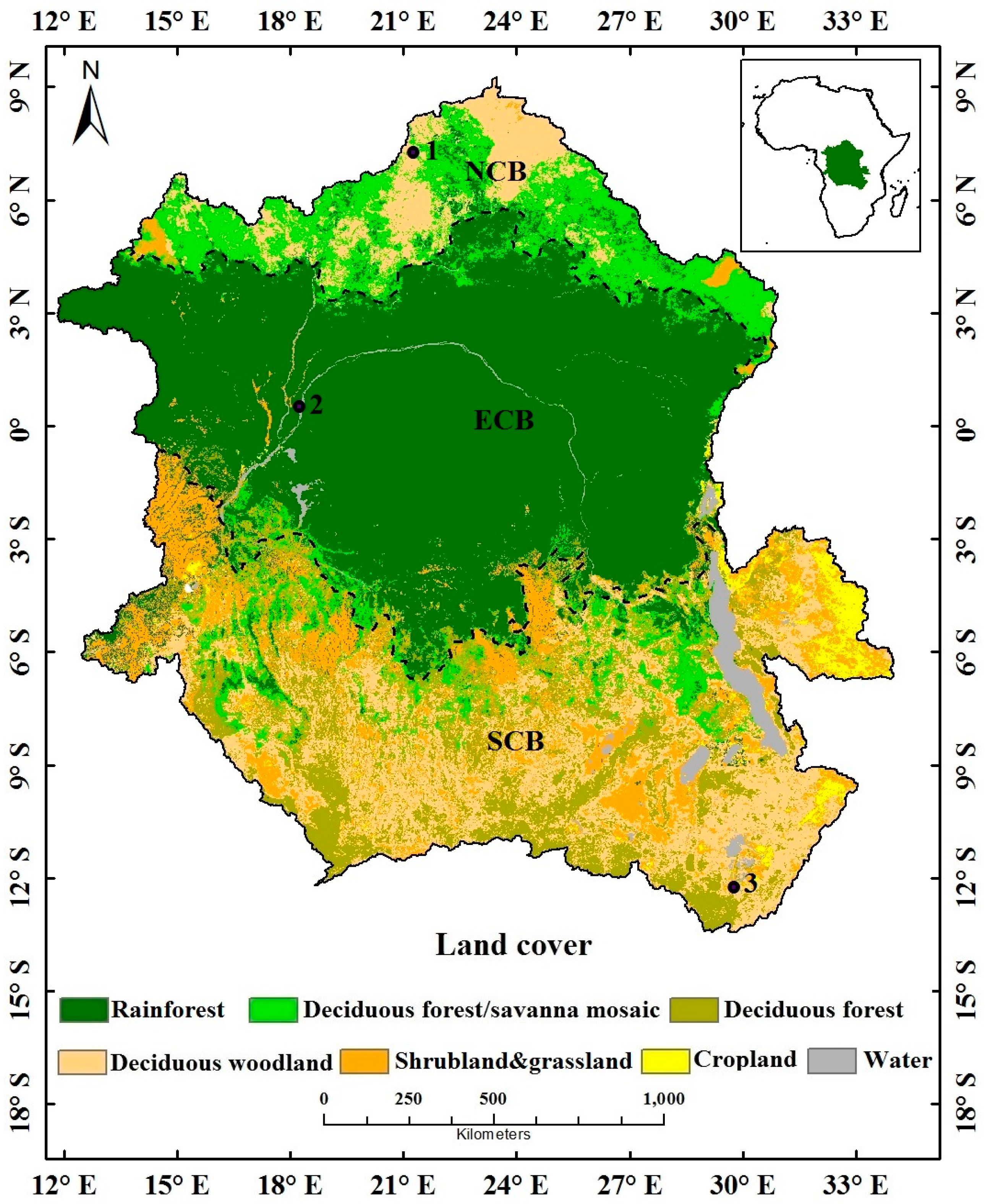
We extracted land cover information from the 1 km land cover product of Africa generated by the Global Land Cover 2000 project (http://forobs.jrc.ec.europa.eu/products/glc2000/products.php) [21] (Figure 2). We chose the Global Land Cover 2000 product instead of other products [14,26,27] due to the following considerations. First, the Global Land Cover 2000 product relies on knowledge from local experts and remotely sensed data from both optical and microwave sensors, which is more suitable for cloud-prone regions such as the Congo Basin, rather than the products derived from data mainly acquired by optical sensors, such as the Moderate Resolution Imaging Spectroradiometer and the Medium Resolution Imaging Spectrometer [14,21,27]. The Global Land Cover 2000 product has an overall accuracy of 68.6% according to sample sites collected around the world [28], and it has the highest overall accuracy (56%) among five satellite-derived land cover products in Africa [29]. Second, the GLC200 product provides a more detailed classification scheme than that offered by the product from the Moderate Resolution Imaging Spectroradiometer, which allows us to examine the differences in the LSP response to the rainy season across land cover types. Based on the mean fractional tree cover reported in [21], we obtained the following land cover groups: grassland and shrubland (GRS) (fractional tree cover < 20%), deciduous woodland and deciduous forest (DWF) (fractional tree cover = ~30%), deciduous forest and savanna mosaic (DFS) (fractional tree cover = ~43%) and tropical rainforest (TRF) (fractional tree cover > 50%). The area covered by cropland and water was excluded from the following analyses.
3.2. Detection of the Rainy Season from Tropical Rainfall Measurement Mission Product
We employed the daily rainfall time series derived from the Tropical Rainfall Measurement Mission product (3B42, Version 7) during 1998–2013 to detect the yearly onset and end of the rainy season. The Tropical Rainfall Measurement Mission product provides global measurements of three-hourly rainfall rates (mm/h) between 50°N and 50°S at 0.25° resolution [30]. Daily rainfall was generated by summing up the three-hourly rainfall based on the measured rainfall rate. The onset and end of the rainy season (hereafter referred to as ORS and ERS, respectively) in Africa have been previously determined using a suite of algorithms [8,11,12,19,31]. For example, ORS and ERS can be determined using a pre-defined threshold of the cumulative rainfall over a fixed time period [8,11,12,31]. Alternatively, yearly ORS and ERS can be determined based on climatological anomalous accumulation (CAA), which refers to the accumulation of the difference between the long-term daily average rainfall and the mean value across the daily average rainfall time series [19]. We adopted this method for the rainy season detection in this study and refer to this method as the CAA method hereafter. The details are provided in the following paragraphs.
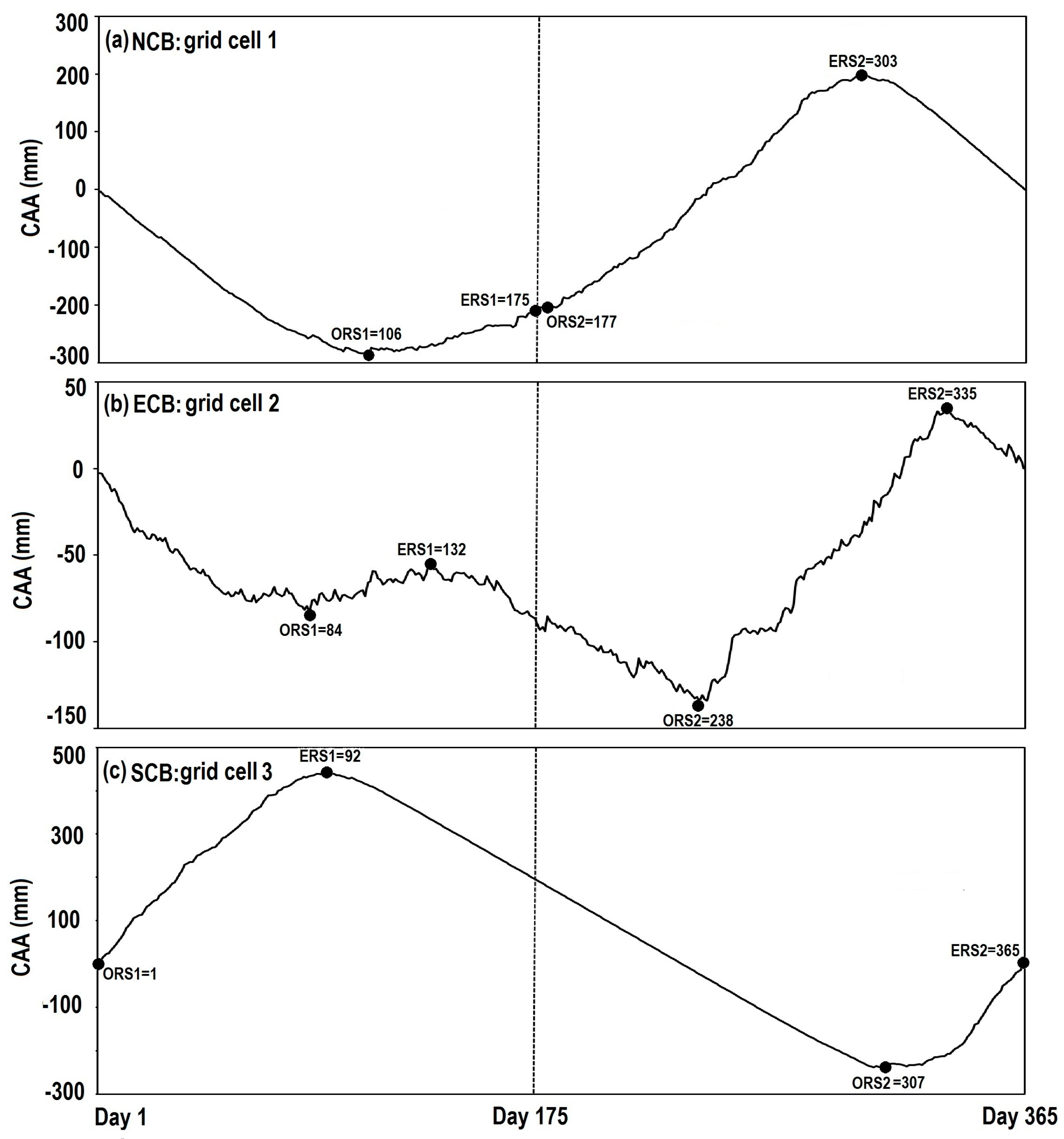
To determine ORS and ERS for a given year, the climatological ORS and ERS were first determined based on the following steps [19]. (1) For each day of a year, the daily average rainfall was calculated using rainfall on the same day but in different years during 1998–2013. (2) The annual-mean rainfall was calculated as the mean value across the daily average rainfall time series. (3) The climatological anomalous rainfall for each day was determined by deducting the annual-mean rainfall from the daily average rainfall. The CAA time series was then generated by accumulating the climatological anomalous rainfall across the year. (4) Since the CAA method was originally designed to detect the rainy season in regions with a unimodal rainfall regime, we modified the CAA method to accommodate the bimodal rainfall regime in ECB. The original CAA method determines the climatological ORS and ERS as the first day after the minimum and maximum CAA, respectively [19]. Based on an exhaustive visual examination of the CAA time series extracted from individual grid cells in ECB, we found that the two rainy seasons could be separated using day 175. We therefore modified the CAA method by first dividing the CAA time series into two sections: day 1–175 and day 176–365 (Figure 3). For each section, we first identified all the days corresponding to a local CAA minimum. We then determined ORS as the first day after the local minimum that has the lowest CAA within this section. ERS was thereafter determined as the first day after the maximum CAA between ORS and the last day of this section. As a result, there were two potential ORS and ERS for each 0.25° grid cell (Figure 3). (5) To determine the rainfall regime for a grid cell, we calculated the number of days during the two potential dry seasons: ERS1 to ORS2 and ERS2 to ORS1. Our premise was that if a given grid cell has a bimodal regime, it must have two relatively long dry seasons such as in Figure 3b. A unimodal regime can be determined if one potential dry season is long, whereas the other one is short, such as in Figure 3a,c. (6) Based on all the 0.25° grid cells in ECB, we generated two dry season length thresholds, which were the average number of days from ERS1 to ORS2 and from ERS2 to ORS1. (7) Finally, if the duration of both potential dry seasons were longer than the corresponding threshold, a bimodal rainfall regime was determined, and the two potential ORS and ERS were employed as the climatological ORS and ERS, respectively. If the duration of one potential dry season was shorter than the corresponding threshold, a unimodal rainfall regime was determined. The potential ORS and ERS associated with this short dry season were ignored. The remaining ORS and ERS were used as the climatological ORS and ERS.
Yearly ORS and ERS were then retrieved using the following procedures [19]. (1) For each year, we defined a rainy season search time period that begins at 50 days prior to climatological ORS and ends at 50 days after climatological ERS. The 50-day buffer was used to deal with the variability in yearly ORS and ERS. For the grid cells with a bimodal rainfall regime, there were two search time periods per year. (2) For each day within the search time period, we calculated the anomalous rainfall by subtracting the long term annual-mean rainfall from the daily rainfall. (3) We generated an accumulated anomalous rainfall time series by accumulating anomalous rainfall throughout the search interval. (4) Yearly ORS and ERS was determined as the first day past the minimum and maximum accumulated anomalous rainfall, respectively. We calculated the mean values and standard deviations in the rainy season timings using the yearly ORS and ERS at the 0.25° grid cells where yearly ORS and ERS were detected in at least four years during 2006–2013.
3.3. Generation of Angularly Corrected Vegetation Index and Detection of Canopy Creenness Cycles
SEVIRI is one of the Earth observation instruments carried by the METEOSAT Second Generation geostationary satellites, with the nadir falling on the equator at the 0° longitude. It delivers a full-disk scan every 15 min, covering Africa, and parts of Europe and South America with a pixel size of 3 km at nadir. The pixel size increases with satellite zenith angle [32]. We generated the Two-band Enhanced Vegetation Index (EVI2) every 30 min based on Equation (1) [33].
In (1), RED and NIR represent the reflectance in red and near infrared channels respectively. EVI2 outperforms NDVI by exhibiting higher sensitivity over densely vegetated canopies [34], which makes it more suitable for vegetation change monitoring in regions such as the Congo Basin. In order to minimize the EVI2 variations caused by changes in sun-satellite geometry, we converted each 30-min EVI2 to an EVI2 obtained under a reference sun-satellite geometry (), in which is the solar zenith angle, is the satellite zenith angle and is the sun-satellite relative azimuth angle. This conversion was done by using an empirical kernel-driven model proposed for SEVIRI [35] as shown in Equation (2).
In (2), is the predicted EVI2 under the reference sun-satellite geometry (). is the observed EVI2 at time . C0 and C1 are kernel weights, which are −0.0723 and −0.0101 for SEVIRI, respectively [35]. FS and FR represent the kernel function that models EVI2 changes caused by sun-satellites in solar and satellite zenith angles, and the sun-satellite relative azimuth angle, respectively [35]. We further determined the daily angularly corrected EVI2 as the maximum angularly corrected 30-minunte EVI2 obtained within a day with solar zenith angle being less than 60°.
According to a previous study on LSP retrieval uncertainty in Congo Basin, a three-day EVI2 time series from SEVIRI is able to provide sufficient cloud-free data for LSP retrieval purposes [16]. In order to reduce data volume while retaining a fine temporal resolution for CGC detection, we composited the daily angularly-corrected EVI2 into a three-day EVI2 time series by extracting the maximum EVI2 acquired under cloud-free conditions. There were 122 three-day EVI2 composites in each year during 2006–2013. To detect CGC, the three-day EVI2 time series was first smoothed using the Savitzky–Golay filter, and a local median filter that removed gaps and irregular values resulting from cloud contamination and other noises [36]. The EVI2 temporal trajectory was then reconstructed by fitting logistic curves to the smoothed EVI2 time series using the Hybrid Piecewise Logistic Model [36]. The rate of change in the curvature of the reconstructed EVI2 temporal trajectory was further calculated. Finally, CGC onset corresponds to the first local maximum of the rate of change in curvature during the ascending phase of the EVI2 trajectory, whereas CGC end corresponds to the last local minimum of the rate of change in curvature during the descending phase [37].
3.4. Investigation of Land Cover Impacts on LSP Responses to the Rainy Season
Since the pixel size of SEVIRI varies with satellite zenith angle, we first aggregated the detected CGC onset and end to 0.25° grids to make them spatially compatible with ORS and ERS. We adopted the aggregation method developed by a previous study on the relationship between vegetation phenology and rainfall seasonality in Africa [12]. Specifically, for a given 0.25° grid cell, we began by sorting the enclosed SEVIRI pixels in ascending order based on the detected CGC onset date. We then identified a 60-day period that includes the highest number of SEVIRI pixels. Finally, we calculated the CGC onset date for this 0.25° grid cell as the average CGC onset date from the SEVIRI pixels falling in the 60-day period. The CGC end date was aggregated to 0.25° grids in the same manner. In this way, the irregular CGC onset/end values exhibited by non-dominant land cover types were excluded from the aggregation, which reduced impacts from mixed land cover. We also calculated the mean values and standard deviations in CGC onset and CGC end for each 0.25° grid cell where CGC onset and CGC end were detected in at least four years during 2006–2013.
To analyze land cover impacts on the responses of LSP to the rainy season, we aggregated the 1 km land cover product to 0.25°, to spatially match the detected rainy season and CGC metrics. The land cover for a given 0.25° grid cell was determined as the dominant land cover among all the 1 km pixels that fell in this 0.25° grid cell. Based on the aggregated land cover map, we randomly selected a grid cell from deciduous woodland in NCB, tropical rainforest in ECB, and grassland in SCB (denoted as black dots in Figure 2), respectively, to demonstrate the changes in the temporal patterns of CGC and rainy season across the study area.
We further examined the variation in the timing difference between CGC and the rainy season across the four land cover groups described in Section 3.1 in each year during 2006–2013. For any given year, this was done by comparing the cumulative distribution function (CDF) of the timing difference extracted from the 0.25° grid cells of any two land cover groups. In order to determine if the CDF of CGC onset lead time (i.e., CGC onset–ORS) from two land cover groups was significantly different, we conducted a one-tailed two-sample Kolmogorov-Smirnov test using the R package “dgof” [38]. Taking the Kolmogorov-Smirnov test between the CDF of CGC onset lead time from grassland and shrubland (GRS) and that from deciduous forest and savanna mosaic (DFS) as an example (i.e., CDFGRS and CDFDFS) (Figure 4a), the null hypothesis was that CDFDFS is larger than or equal to CDFGRS. By rejecting the null hypothesis, the alternative hypothesis is accepted that CDFDFS is smaller than CDFGRS, which means that CDFDFS stays above and to the left of CDFGRS. For example, in Figure 4a, the number of grid cells with a CGC onset lead time less than −50 (i.e., CGC onset occurs 50 days or more prior to ORS) accounted for 17% of the grid cells from GRS, whereas it accounted for as much as 46% from DFS. In other words, CGC onset in DFS preceded ORS by a larger number of days than CGC onset did in GRS, which made CDFDFS “numerically” smaller than CDFGRS. This analysis was repeated to investigate the impacts of land cover on CGC end lag time relative to ERS (i.e., CGC end−ERS). In Figure 4b, for example, the number of grid cells with a CGC lag time less than 50 (i.e., CGC end lags behind ERS for 50 days or less) only accounted for 21% of the grid cells in GRS whereas it accounted for as much as 61% of the grid cells in DFS. This indicates that the grid cells with a shorter lag time had a higher percentage in DFS than it did in GRS. Therefore, CDFDFS is “numerically” smaller than CDFGRS.
We also conducted a linear regression analysis with the spatial variation in ORS and CGC onset being the predictor and response variable, respectively. This regression analysis was conducted for each type of land cover separately in each year during 2006–2013. The regression analyses were performed in R, and we retrieved the number of samples, R-square value, and the residual standard error for each regression analysis. Specifically, for the regression analysis involving a particular type of land cover in a specific year, the number of samples was determined as the number of 0.25° grid cells with this land cover where both CGC onset and ORS were detected in that year. The regression analyses were also repeated between ERS and CGC end. We did not conduct the regression analyses on a per-grid basis, because, for each 0.25° grid cell, we only had eight sample pairs of the CGC and the rainy season timings at most, which were too few samples for statistically robust regression analyses.
4. Results
4.1. Inter-Annual Variations in the Timings of Both the Rainy Season and CGC
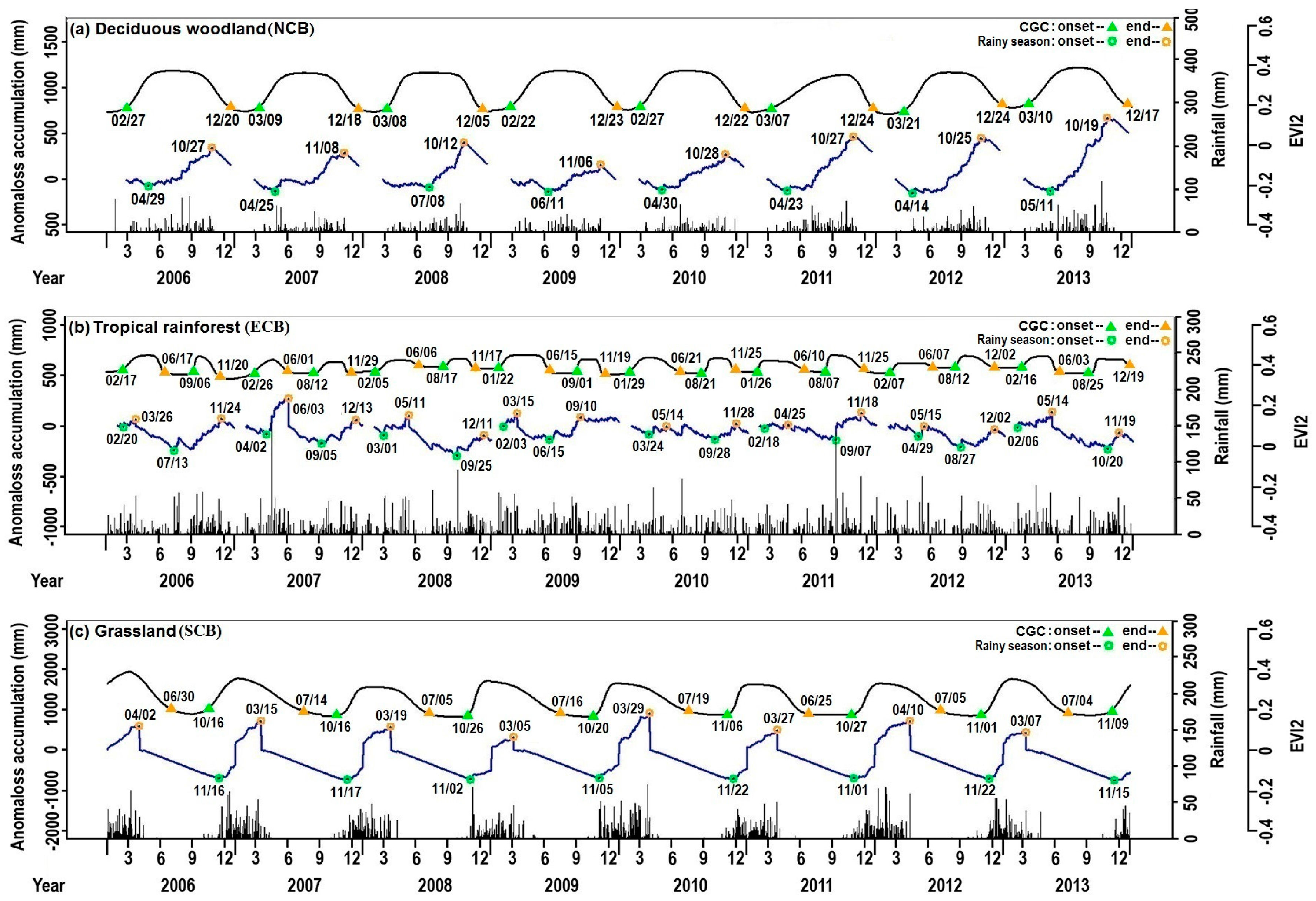
Figure 5 presents the inter-annual variations in the rainy season and CGC at the three selected grid cells denoted in Figure 2. The rainy season at the deciduous woodland and grassland grid cells was regulated by distinct unimodal regimes whereas it was associated with a bimodal regime at the rainforest grid cell. These rainfall regimes affected the seasonal pattern of CGC variation. At the deciduous woodland grid cell, CGC onset occurred much earlier than ORS. The average lead time of CGC onset was 67 days, with a minimum and maximum of 24 and 122 days in 2012 and 2008, respectively. Although CGC onset also occurred earlier than ORS at the grassland grid cell, the CGC onset lead time was relatively small, which varied from five days in 2011, to 32 days in 2007, with an average of 17 days during 2006–2013. At the rainforest grid cell, CGC onset occurred prior to ORS in most years. Specifically, the first CGC onset occurred earlier than ORS in all years except 2013, whereas the second CGC onset lagged behind ORS only in 2006 and 2009. The average lead time of the first and second CGC onset was 28 and nine days, respectively, during 2006–2013. In contrast to CGC onset, CGC end substantially lagged behind ERS in most years at the selected grid cells. The longest lag was found at the grassland grid cell, where lag duration ranged from 86 (year 2012) to 133 (year 2009) days, with an average of 107 days. Moderate lag was found at the deciduous woodland grid cell where CGC end lagged behind ERS by an average of 53 days. The minimum lag was 40 days in 2007, whereas the maximum lag was 60 days in 2012. At the rainforest grid cell, the average lag duration for the first and second CGC end was 41 and eight days, respectively. The short average lag duration for the second CGC end resulted from the high inter-annual variations. Specifically, the second CGC end occurred 24 days before ERS in 2008, whereas it lagged behind ERS by as much as 70 days in 2009.
4.2. Spatial Patterns of the Rainy Season and CGC Timings
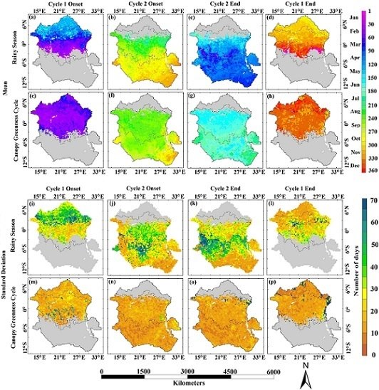
Figure 6 presents the spatial patterns of the mean value and standard deviation in the rainy reason and CGC timings during 2006–2013. The spatial variations in the mean values of ORS and ERS exhibited distinct latitudinal gradients. The first cycle of the rainy season occurred in ECB and NCB, whereas the second cycle occupied the ECB and SCB. ORS exhibited delays, whereas ERS showed advances toward higher latitudes in both cycles. ORS in the first cycle varied from early Febuary to late May, whereas the second cycle ORS varied from mid-August to mid-November. ERS in the first and second cycle occurred between mid-October and late December, and between mid-March and mid-June, respectively. In contrast, the spatial variations in CGC timing were not as strong as those during rainy season timing. CGC onset predominately occurred around mid-Feburary and early September in the first and second cycle, respectively. CGC ended around mid-December over much of ECB and NCB in the first cycle, whereas it predominately ended during June–July in the second cycle across ECB and SCB. The most pronounced timing difference between ORS and CGC onset was observed in NCB and SCB, where CGC onset substantially preceded ORS. CGC end lagged behind ERS over much of the Congo Basin in both cycles. The area with double annual CGCs was more widespread than the area with two annual rainy seasons. Standard deviation in rainy season timings exhibited high spatial heterogeneity, whereas it was relatively homogeneous in CGC timings across the Congo Basin. The standard deviation was higher in the rainy season timings than in CGC timings over much of the Congo Basin. Specifically, the standard deviation in both ORS and ERS could be more than 40 days in some areas, whereas it was predominatly less than 20 days in CGC timings.
4.3. Impacts of Land Cover on the Responses of CGC Timing to the Rainy Season
Figure 7 presents the variations in the timing differences between CGC and the rainy season among the four land cover groups. For each year in 2006–2013, based on KS tests, we identified the following relationship for CGC onset lead time: CDFDFS < CDFDWF < CDFGRS (p < 0.001) and CDFDFS < CDFTRF (p < 0.001). In other words, the length of time by which CGC onset precedes ORS increased with tree cover from grassland and shrubland (GRS) to deciduous forest and savanna mosaic (DFS). After CGC onset lead time reached the maximum in DFS, it started to decrease toward the region covered by tropical rainforest (TRF). For the time difference between CGC end and ERS, we found the following relationship in all years during 2006–2013: CDFTRF < CDFDFS < CDFDWF ≈ CDFGRS (p < 0.001). In other words, the length of time by which CGC end lagged behind ERS, became longer toward the groups with lower tree cover.
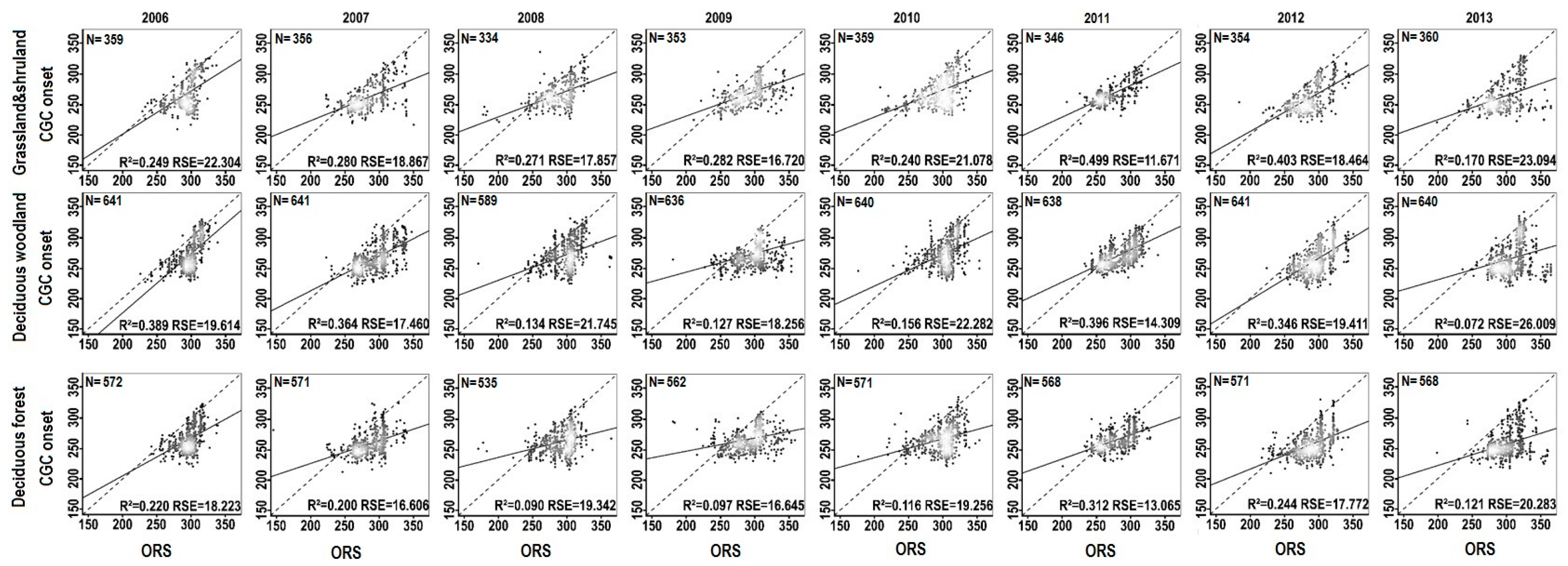
Figure 8 shows the results from the regression analyses between the spatial variations in the rainy season timing and in CGC. During 2006–2013, we identified the significant relationships between ORS and CGC onset (p < 0.001) in grassland and shrubland, deciduous woodland and deciduous forest. The R2 value from the regressions between ORS and CGC onset increased with decreases in tree cover during 2008–2013. The only exception was found in 2013, when the R2 for deciduous forest was higher than that of deciduous woodland. In both 2006 and 2007, deciduous woodland and deciduous forest had the highest and lowest R2 values, respectively. We did not identify any significant relationship between the spatial variations in ERS and that of CGC end for any types of land cover during 2006–2013.
5. Discussion
5.1. The Regulation of the Rainy Season by Intertropical Convergence Zone and the Detection of Rainy Season Using the CAA Method
The migration of intertropical convergence zone follows the movements of the solar zenith point over the year [19,39]. The intertropical convergence zone initiates northward migration in early February, which triggers the first ORS in ECB. The continuous movement of intertropical convergence zone toward northern latitudes initiates the single rainy season in NCB. Meanwhile, ECB becomes relatively dry, and the first ERS begins to commence. After reaching the northern limit in the boreal summer, the intertropical convergence zone starts to retreat and move toward the southern hemisphere. The intertropical convergence zone moves across ECB and SCB, which triggers the second ORS in ECB and the onset of the single rainy season in SCB. As the intertropical convergence zone moves further south after crossing SCB, ERS in NCB and the second ERS in ECB begin to commence. After reaching the southern limit in the austral summer, the intertropical convergence zone starts to move northward again [39], which initiates a new cycle of the rainy season in ECB and NCB and triggers ERS within SCB.
The spatial variations in the rainy season timings determined in our study generally agree with those determined for NCB and SCB from previous studies [11,12,19]. The CAA method has both advantages and disadvantages in rainy season detection, compared with other methods. The advantages of the CAA method are as follows. (1) It does not require the rainfall thresholds that have been well-tested for a certain type of vegetation or a certain region. For example, in the studies by Ryan et al. [8] and Brown and de Beurs [31], ORS is determined when a minimum of 25 mm rainfall has been accumulated in a 10-day period, followed by at least 20 mm rainfall accumulation in the next 20 days. Those thresholds are recommended by studies on the rainfall control over crop growth [40,41]. Since no recommended thresholds are available for most types of land cover in the Congo Basin, the CAA method is a better choice from this perspective. (2) The CAA method is less affected by isolated bursts of heavy rainfall when determining ORS and ERS. In a previous study on the hydrological controls of LSP in Africa’s savannas and woodlands, ORS is determined when the cumulative rainfall exceeds 5% or 10% of the mean annual rainfall [11]. If this method was applied for the year of 2006 or 2009 in Figure 5a, a false ORS would have been obtained due to the isolated bursts of heavy rainfall prior to the true ORS. The disadvantage of CAA method is that a slight change in the anomalous rainfall time series can result in substantial differences in detecting the rainy season timing. In Figure 5a, for instance, the anomalous rainfall time series reached a local minimum of −88.29 mm on 13 April 2008, which was close to the ORS over most of the years (i.e., 2006, 2007 and 2010–2012). However, due to a short dry spell between mid-June and early July, the anomalous rainfall time series reached another local minimum of −94.02 mm on July 7, the next day of which was determined as the ORS in 2008. Therefore, a difference of 5.73 mm in anomalous rainfall accumulation between April 13 and July 8 resulted in a difference of 81 days in ORS. This issue should be addressed in future studies by introducing a reasonable range of minimum anomalous rainfall, which would allow multiple candidate ORS dates to be evaluated based on both the anomalous rainfall and their deviation from the long-term mean.
The bimodal rainfall regime was only found within the central ECB, whereas double annual CGCs were found across almost the entire ECB. This mismatch is caused by the threshold method we employed to differentiate between unimodal and bimodal rainfall regimes. Since rainfall regime varies continuously across space, rainfall regimes in the grid cells within northern and southern ECB exhibit a transitional status between unimodal and bimodal, with the duration of one of the two potential dry seasons being shorter than the average from ECB. Although a unimodal rainfall regime was determined for those grid cells using our method, canopy greenness still responds to this transitional rainfall regime by exhibiting two annual cycles.
5.2. The Impacts of Land Cover on the Responses of CGC to the Rainy Season
Rainfall is the dominant limiting factor of canopy greenness in the Congo Basin [6,42,43]. This can be explained by that, compared to other regions dominated by tropical forests such as the Amazon Basin and Southeast Asia, the Congo Basin receives less rainfall during the rainy season. Decreases in canopy greenness occur during the dry season due to limited water storage surplus from the preceding rainy season [42,43]. As a result, CGC in the Congo Basin follows alternations of wet and dry periods. However, the timing discrepancy between the rainy season and CGC was apparent. Results from our study indicated that CGC onset occurs prior to ORS mainly in areas occupied by forests and woodlands whereas CGC end lags behind ERS across much of the Congo Basin, which agreed with the findings by previous studies based on remotely sensed LSP and rainfall data [8,11]. Early CGC onset in tropical forests and woodlands has been documented in numerous studies [8,11,44,45,46,47]. The suggested underlying mechanisms include the utilization of groundwater and stem-water reserve during the dry season by tropical trees [8,11,44,47], and that CGC onset of tropical trees is cued by insolation instead of rainfall [8]. The inter-annual variation in CGC onset is predominately less than 20 days, which is comparable with the inter-annual variation of about 10 days derived from a previous study [8]. This low inter-annual variation in CGC onset might result from the cue by insolation, which has low inter-annual variation in the tropics [8,11]. The response of CGC onset to ORS became stronger with decreases in tree cover. This was shown by the decreases in CGC onset lead time and the stronger spatial relationship between ORS and CGC onset from deciduous forests to grassland and shrubland. In other words, the effectiveness of using ORS to predict CGC onset increased toward the land cover with lower tree cover. This is because CGC onset in grassland depends on soil moisture in the surface layer, which can only be recharged shortly prior to, or after ORS [44]. The lag of CGC end behind ERS can be explained by the existence of rainfall events after ERS, as well as the availability of groundwater and stem-water reserves during the dry season [11]. Moreover, ERS has a stronger correspondence with the onset of canopy greenness decrease, instead of with canopy greenness minimum (i.e., CGC end) [11]. Both the CGC onset lead time and CGC end lag time showed decreases toward ECB occupied by tropical rainforests. It is likely that the decreases in timing difference are related to the saturated impact by rainy season length on CGC length, which refers to the limited increases in CGC length, given substantial increases in rainy season length from the surrounding areas of the ECB, to the ECB itself. This saturated impact has been reported for the transitional regions between deciduous forests and evergreen rainforests in the Congo Basin [11].
6. Conclusions
In this study, we investigated the effects of land cover on the relationship between CGC timing and the rainy season timing in the Congo Basin during 2006–2013. We were able to reveal the changes in the modality of rainfall and CGC across the Congo Basin using a time series of remotely sensed rainfall and EVI2.
The response of CGC timing to that of the rainy season was a function of land cover. The CGC onset lead time prior to ORS was longer in tropical woodlands and forests, whereas it became relatively short in grasslands and shrublands. Further, the spatial variation in CGC onset had a stronger correlation with that of ORS in grasslands and shrublands, than in tropical woodlands and forests. This suggests that ORS has stronger control over CGC onset in regions with lower tree cover, while the CGC onset of tropical trees is likely to be associated with deep ground water, stem-water reserves, and insolation in a complex manner. In contrast, the lag of CGC end behind ERS was widespread across the Congo Basin, which was longer in grasslands and shrublands than in tropical woodlands and forests. However, no significant relationship was identified between spatial variations in ERS and CGC end. The spatial and inter-annual variations in CGC timing were relatively small compared with variations in the rainy season timing. Overall, CGC in the Congo Basin follows the alternation of wet and dry period, but the underlying mechanism is complex and varies with land cover.
Acknowledgments
This study was supported by the NOAA GOES-R Risk Reduction Project GOES-R3#250, the NOAA contract JPSS_PGRR2_14 and NASA contracts NNX15AB96A. All the code used in this manuscript can be accessed by contacting the corresponding author and the datasets in this study will be made available via http://openprairie.sdstate.edu/.
Author Contributions
Dong Yan and Xiaoyang Zhang conceived and designed the experiments; Dong Yan, Yunyue Yu and Wei Guo analyzed the data; Dong Yan and Xiaoyang Zhang wrote the paper.
Conflicts of Interest
The authors declare no conflict of interest.
Abbreviations
| CAA | Climatological Anomalous Accumulation |
| CDF | Cumulative Distribution Function |
| CGC | Canopy Greenness Cycle |
| DFS | Deciduous Forest and Savanna Mosaic |
| DWF | Deciduous Woodland and Deciduous Forest |
| ECB | Equatorial Congo Basin |
| ERS | End of Rainy Season |
| EVI2 | Two-band Enhanced Vegetation Index |
| GRS | Grassland and Shrubland |
| LSP | Land surface phenology |
| NCB | Northern Congo Basin |
| ORS | Onset of Rainy Season |
| SCB | Southern Congo Basin |
| SEVIRI | Spinning Enhanced Visible and Infrared Imager |
| TRF | tropical rainforest |
References
- Phillips, O.L.; Malhi, Y.; Higuchi, N.; Laurance, W.F.; Núñez, P.V.; Vásquez, R.M.; Laurance, S.G.; Ferreira, L.V.; Stern, M.; Brown, S.; et al. Changes in the carbon balance of tropical forests: Evidence from long-term plots. Science 1998, 282, 439–442. [Google Scholar] [CrossRef] [PubMed]
- Malhi, Y.; Adu-Bredu, S.; Asare, R.A.; Lewis, S.L.; Mayaux, P. African rainforests: Past, present and future. Philos. Trans. R. Soc. B Biol. Sci. 2013, 368, 20120312. [Google Scholar] [CrossRef] [PubMed]
- Megevand, C.; Mosnier, A.; Hourticq, J.; Sanders, K.; Doetinchem, N.; Streck, C. Deforestation Trends in the Congo Basin: Reconciling Economic Growth and Forest Protection; World Bank: Washington, DC, USA, 2013. [Google Scholar]
- De Wasseige, C.; De Marcken, P.; Bayol, N.; Hiol Hiol, F.; Mayaux, P.; Desclée, B.; Nasi, R.; Billand, A.; Defourny, P.; Eba’a Atyi, R. The Forests of the Congo Basin—State of the Forest 2010; Publications Office of the European Union: Luxembourg, 2012. [Google Scholar]
- Asefi-Najafabady, S.; Saatchi, S. Response of african humid tropical forests to recent rainfall anomalies. Philos. Trans. R. Soc. B Biol. Sci. 2013, 368, 20120306. [Google Scholar] [CrossRef] [PubMed]
- Zhou, L.; Tian, Y.; Myneni, R.B.; Ciais, P.; Saatchi, S.; Liu, Y.Y.; Piao, S.; Chen, H.; Vermote, E.F.; Song, C.; et al. Widespread decline of congo rainforest greenness in the past decade. Nature 2014, 509, 86–90. [Google Scholar] [CrossRef] [PubMed]
- Fauset, S.; Baker, T.R.; Lewis, S.L.; Feldpausch, T.R.; Affum-Baffoe, K.; Foli, E.G.; Hamer, K.C.; Swaine, M.D. Drought-induced shifts in the floristic and functional composition of tropical forests in ghana. Ecol. Lett. 2012, 15, 1120–1129. [Google Scholar] [CrossRef] [PubMed]
- Ryan, C.M.; Williams, M.; Grace, J.; Woollen, E.; Lehmann, C.E.R. Pre-rain green-up is ubiquitous across southern tropical africa: Implications for temporal niche separation and model representation. New Phytol. 2017, 213, 625–633. [Google Scholar] [CrossRef] [PubMed]
- Buitenwerf, R.; Rose, L.; Higgins, S.I. Three decades of multi-dimensional change in global leaf phenology. Nat. Clim. Chang. 2015, 5, 364–368. [Google Scholar] [CrossRef]
- De Beurs, K.M.; Henebry, G.M. War, drought, and phenology: Changes in the land surface phenology of afghanistan since 1982. J. Land Use Sci. 2008, 3, 95–111. [Google Scholar] [CrossRef]
- Guan, K.; Wood, E.F.; Medvigy, D.; Kimball, J.; Pan, M.; Caylor, K.K.; Sheffield, J.; Xu, X.; Jones, M.O. Terrestrial hydrological controls on land surface phenology of african savannas and woodlands. J. Geophys. Res. Biogeosci. 2014, 119, 1652–1669. [Google Scholar] [CrossRef]
- Zhang, X.; Friedl, M.A.; Schaaf, C.B.; Strahler, A.H.; Liu, Z. Monitoring the response of vegetation phenology to precipitation in africa by coupling modis and trmm instruments. J. Geophys. Res. Atmos. 2005, 110, D12103. [Google Scholar] [CrossRef]
- Gond, V.; Fayolle, A.; Pennec, A.; Cornu, G.; Mayaux, P.; Camberlin, P.; Doumenge, C.; Fauvet, N.; Gourlet-Fleury, S. Vegetation structure and greenness in central africa from modis multi-temporal data. Philos. Trans. R. Soc. B Biol. Sci. 2013, 368, 20120309. [Google Scholar] [CrossRef] [PubMed]
- Verhegghen, A.; Mayaux, P.; De Wasseige, C.; Defourny, P. Mapping congo basin vegetation types from 300 m and 1 km multi-sensor time series for carbon stocks and forest areas estimation. Biogeosciences 2012, 9, 5061–5079. [Google Scholar] [CrossRef]
- Guan, K.; Medvigy, D.; Wood, E.F.; Caylor, K.K.; Shi, L.; Su-Jong, J. Deriving vegetation phenological time and trajectory information over africa using seviri daily lai. IEEE Trans. Geosci. Remote Sens. 2014, 52, 1113–1130. [Google Scholar] [CrossRef]
- Yan, D.; Zhang, X.; Yu, Y.; Guo, W. A comparison of tropical rainforest phenology retrieved from geostationary (seviri) and polar-orbiting (modis) sensors across the congo basin. IEEE Trans. Geosci. Remote Sens. 2016, 54, 4867–4881. [Google Scholar] [CrossRef]
- Sobrino, J.S.; Julien, Y.; Soria, G. Phenology estimation from meteosat second generation data. IEEE J. Sel. Top. Appl. Earth Obs. Remote Sens. 2013, 6, 1653–1659. [Google Scholar] [CrossRef]
- Herrmann, S.M.; Mohr, K.I. A continental-acale classification of rainfall seasonality regimes in africa based on gridded precipitation and land surface temperature products. J. Appl. Meteorol. Climatol. 2011, 50, 2504–2513. [Google Scholar] [CrossRef]
- Liebmann, B.; Bladé, I.; Kiladis, G.N.; Carvalho, L.M.V.; Senay, G.B.; Allured, D.; Leroux, S.; Funk, C. Seasonality of african precipitation from 1996 to 2009. J. Clim. 2012, 25, 4304–4322. [Google Scholar] [CrossRef]
- Washington, R.; James, R.; Pearce, H.; Pokam, W.M.; Moufouma-Okia, W. Congo basin rainfall climatology: Can we believe the climate models? Philos. Trans. R. Soc. B Biol. Sci. 2013, 368, 20120296. [Google Scholar] [CrossRef] [PubMed]
- Mayaux, P.; Bartholomé, E.; Fritz, S.; Belward, A. A new land-cover map of africa for the year 2000. J. Biogeogr. 2004, 31, 861–877. [Google Scholar] [CrossRef]
- Couralet, C.; Van den Bulcke, J.; Ngoma, L.M.; Van Acker, J.; Beeckman, H. Phenology in functional groups of central african rainforest trees. J. Trop. For. Sci. 2013, 25, 361–374. [Google Scholar]
- Viennois, G.; Barbier, N.; Fabre, I.; Couteron, P. Multiresolution quantification of deciduousness in west-central african forests. Biogeosciences 2013, 10, 6957–6967. [Google Scholar] [CrossRef]
- De Weirdt, M.; Verbeeck, H.; Maignan, F.; Peylin, P.; Poulter, B.; Bonal, D.; Ciais, P.; Steppe, K. Seasonal leaf dynamics for tropical evergreen forests in a process-based global ecosystem model. Geosci. Model Dev. 2012, 5, 1091–1108. [Google Scholar] [CrossRef]
- Myneni, R.B.; Yang, W.; Nemani, R.R.; Huete, A.R.; Dickinson, R.E.; Knyazikhin, Y.; Didan, K.; Fu, R.; Negrón Juárez, R.I.; Saatchi, S.S.; et al. Large seasonal swings in leaf area of amazon rainforests. Proc. Natl Acad. Sci. USA 2007, 104, 4820–4823. [Google Scholar] [CrossRef] [PubMed]
- Friedl, M.A.; Sulla-Menashe, D.; Tan, B.; Schneider, A.; Ramankutty, N.; Sibley, A.; Huang, X. Modis collection 5 global land cover: Algorithm refinements and characterization of new datasets. Remote Sens. Environ. 2010, 114, 168–182. [Google Scholar] [CrossRef]
- Defourny, P.; Vancutsem, C.; Bicheron, P.; Brockmann, C.; Niño, F.; Schouten, L.; Leroy, M.M. Globcover: A 300 m global land cover product for 2005 using envisat meris time series. In Proceedings of the ISPRS Comission VII Mid-Term Symposium: Remote Sensing: From Pixels to Processes, Enschede, The Netherlands, 6 December 2006; pp. 1–4. [Google Scholar]
- Mayaux, P.; Eva, H.; Gallego, J.; Strahler, A.H.; Herold, M.; Agrawal, S.; Naumov, S.; Miranda, E.E.D.; Bella, C.M.D.; Ordoyne, C.; et al. Validation of the global land cover 2000 map. IEEE Trans. Geosc. Remote Sens. 2006, 44, 1728–1739. [Google Scholar] [CrossRef]
- Bai, L. Comparison and Validation of Five Land Cover Products over the African Continent; Lund University: Lund, Sweden, 2010. [Google Scholar]
- Milewski, A.; Elkadiri, R.; Durham, M. Assessment and comparison of tmpa satellite precipitation products in varying climatic and topographic regimes in morocco. Remote Sens. 2015, 7, 5697. [Google Scholar] [CrossRef]
- Brown, M.E.; de Beurs, K.M. Evaluation of multi-sensor semi-arid crop season parameters based on ndvi and rainfall. Remote Sens. Environ. 2008, 112, 2261–2271. [Google Scholar] [CrossRef]
- Fensholt, R.; Sandholt, I.; Stisen, S.; Tucker, C. Analysing ndvi for the african continent using the geostationary meteosat second generation seviri sensor. Remote Sens. Environ. 2006, 101, 212–229. [Google Scholar] [CrossRef]
- Jiang, Z.; Huete, A.R.; Didan, K.; Miura, T. Development of a two-band enhanced vegetation index without a blue band. Remote Sens. Environ. 2008, 112, 3833–3845. [Google Scholar] [CrossRef]
- Huete, A.; Didan, K.; Miura, T.; Rodriguez, E.P.; Gao, X.; Ferreira, L.G. Overview of the radiometric and biophysical performance of the modis vegetation indices. Remote Sens. Environ. 2002, 83, 195–213. [Google Scholar] [CrossRef]
- Tian, Y.; Romanov, P.; Yunyue, Y.; Hui, X.; Tarpley, D. Analysis of vegetation index ndvi anisotropy to improve the accuracy of the goes-r green vegetation fraction product. In Proceedings of the Geoscience and Remote Sensing Symposium (IGARSS), Honolulu, HI, USA, 25–30 July 2010; IEEE: New York, NY, USA, 2010; pp. 2091–2094. [Google Scholar]
- Zhang, X. Reconstruction of a complete global time series of daily vegetation index trajectory from long-term avhrr data. Remote Sens. Environ. 2015, 156, 457–472. [Google Scholar] [CrossRef]
- Zhang, X.; Friedl, M.A.; Schaaf, C.B.; Strahler, A.H.; Hodges, J.C.F.; Gao, F.; Reed, B.C.; Huete, A. Monitoring vegetation phenology using modis. Remote Sens. Environ. 2003, 84, 471–475. [Google Scholar] [CrossRef]
- Arnold, T.B.; Emerson, J.W. Nonparametric goodness-of-fit tests for discrete null distributions. R J. 2011, 3, 34–39. [Google Scholar]
- Haensler, A.; Saeed, F.; Jacob, D. Assessment of projected climate change signals over central africa based on a multitude of global and regional climate projections. In Climate Change Scenarios for the Congo Basin; Climate Service Centre Report No. 11; Haensler, A., Jacob, D., Kabat, P., Ludwig, F., Eds.; Climate Service Center: Hamburg, Germany, 2013. [Google Scholar]
- Tadross, M.A.; Hewitson, B.C.; Usman, M.T. The interannual variability of the onset of the maize growing season over south africa and zimbabwe. J. Clim. 2005, 18, 3356–3372. [Google Scholar] [CrossRef]
- AGRHYMET. Méthodologie de Suivi Des Zones À Risque; Centre Regional AGRHYMET: Niamey, Niger, 1996. [Google Scholar]
- Guan, K.; Pan, M.; Li, H.; Wolf, A.; Wu, J.; Medvigy, D.; Caylor, K.K.; Sheffield, J.; Wood, E.F.; Malhi, Y.; et al. Photosynthetic seasonality of global tropical forests constrained by hydroclimate. Nat. Geosci. 2015, 8, 284–289. [Google Scholar] [CrossRef]
- Guan, K.; Wolf, A.; Medvigy, D.; Caylor, K.K.; Pan, M.; Wood, E.F. Seasonal coupling of canopy structure and function in african tropical forests and its environmental controls. Ecosphere 2013, 4, 1–21. [Google Scholar] [CrossRef]
- Ryan, C.M.; Williams, M.; Hill, T.C.; Grace, J.; Woodhouse, I.H. Assessing the phenology of southern tropical africa: A comparison of hemispherical photography, scatterometry, and optical/nir remote sensing. IEEE Trans. Geosci. Remote Sens. 2014, 52, 519–528. [Google Scholar] [CrossRef]
- Higgins, S.I.; Delgado-Cartay, M.D.; February, E.C.; Combrink, H.J. Is there a temporal niche separation in the leaf phenology of savanna trees and grasses? J. Biogeogr. 2011, 38, 2165–2175. [Google Scholar] [CrossRef]
- Archibald, S.; Scholes, R.J. Leaf green-up in a semi-arid african savanna: Separating tree and grass responses to environmental cues. J. Veg. Sci. 2007, 18, 583–594. [Google Scholar]
- Borchert, R. Soil and stem water storage determine phenology and distribution of tropical dry forest trees. Ecology 1994, 75, 1437–1449. [Google Scholar] [CrossRef]
Figure 1.
A diagram illustrating the procedures for analyzing canopy greenness cycle, rainfall seasonality, and land cover impacts. EVI2: Two-band Enhanced Vegetation Index, CGC: Canopy greenness cycle, CAA: Climatological anomalous accumulation.
Figure 1.
A diagram illustrating the procedures for analyzing canopy greenness cycle, rainfall seasonality, and land cover impacts. EVI2: Two-band Enhanced Vegetation Index, CGC: Canopy greenness cycle, CAA: Climatological anomalous accumulation.
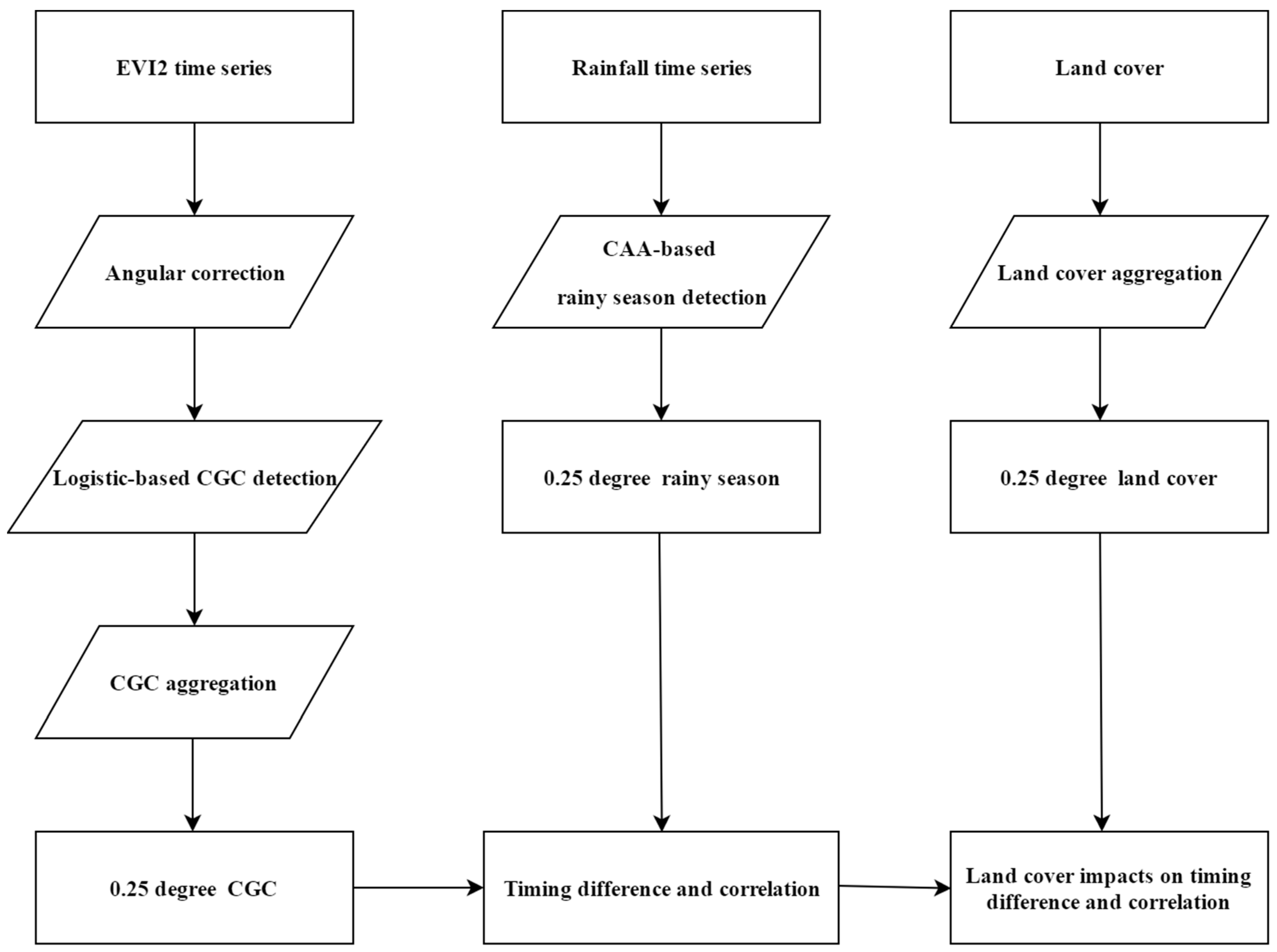
Figure 2.
Land cover types in the Congo Basin extracted from the Global Land Cover 2000 product. Black dots in three grid cells represent deciduous woodland, rainforest and grassland, respectively, which were used to illustrate the analyses of CGC and the rainy season in detail. The dashed lines divide the study area into three sub-basins: Northern Congo Basin (NCB), Eastern Congo Basin (ECB), and Southern Congo Basin (SCB).

Figure 3.
An illustration for determining climatological onset of rainy season (ORS) and end of rainy season (ERS) using the Climatological Anomalous Accumulation (CAA) method. The CAA time series at the deciduous woodland grid cell in NCB (a), the rainforest grid cell in ECB (b) and the grassland grid cell in SCB (c). Grid cells 1 and 3 have a unimodal rainfall regime, whereas grid cell 2 has a bimodal rainfall regime.

Figure 4.
A comparison of the cumulative distribution function for CGC onset lead time (a) and CGC end lag time (b) between grassland and shrubland (GRS) and deciduous forest and savanna mosaic (DFS) land cover groups. The Y-axis represents the percentage of grid cells. The X-axis in (a) represents the number of days that CGC onset precedes ORS, whereas the X-axis in (b) indicates the number of days that CGC end lags behind ERS.
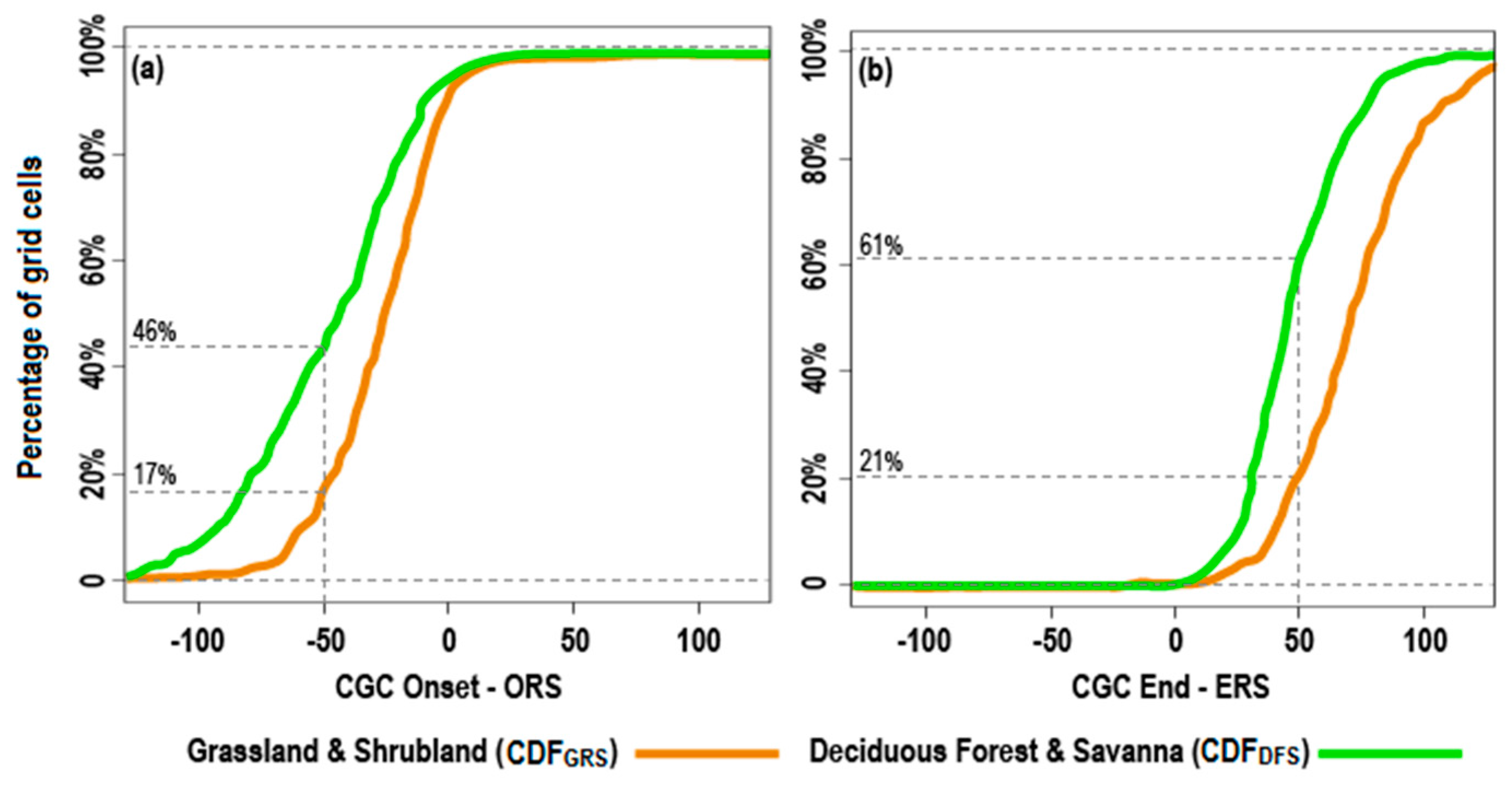
Figure 5.
Inter-annual variations in the rainy season and CGC timing at the deciduous woodland grid cell in NCB (a), the rainforest grid cell in ECB (b) and the grassland grid cell in SCB (c). Black and blue lines represent the reconstructed EVI2 temporal trajectory and the anomalous rainfall accumulation, respectively. Daily rainfall is shown as black bars. Green and orange triangles represent CGC onset and end, respectively. Green and orange circles represent the rainy season onset and end, respectively. The onset and end dates are labeled next to the corresponding symbols using a MM/DD format. The left Y-axis indicates anomalous rainfall accumulation. The first Y-axis on the right represents daily rainfall, whereas the second Y-axis displays EVI2.

Figure 6.
The mean value and standard deviation of the rainy season and CGC timings during 2006–2013 across the Congo Basin. Mean value of rainy season timing (a–d); mean value of CGC timings (e–h); standard deviation of the rainy season timing (i–l); standard deviation of CGC timing (m–p). Note that for areas with two rainy seasons (or CGCs) in ECB, the first rainy season and CGC begin in the first cycle ((a) and (e)) and end in the second cycle ((c) and (g)), whereas the second rainy season and CGC begin in the second cycle ((b) and (f)) and end in the first cycle ((d) and (h)). The gray area indicates that the specific rainy season or CGC metric was detected less than four times during 2006–2013.
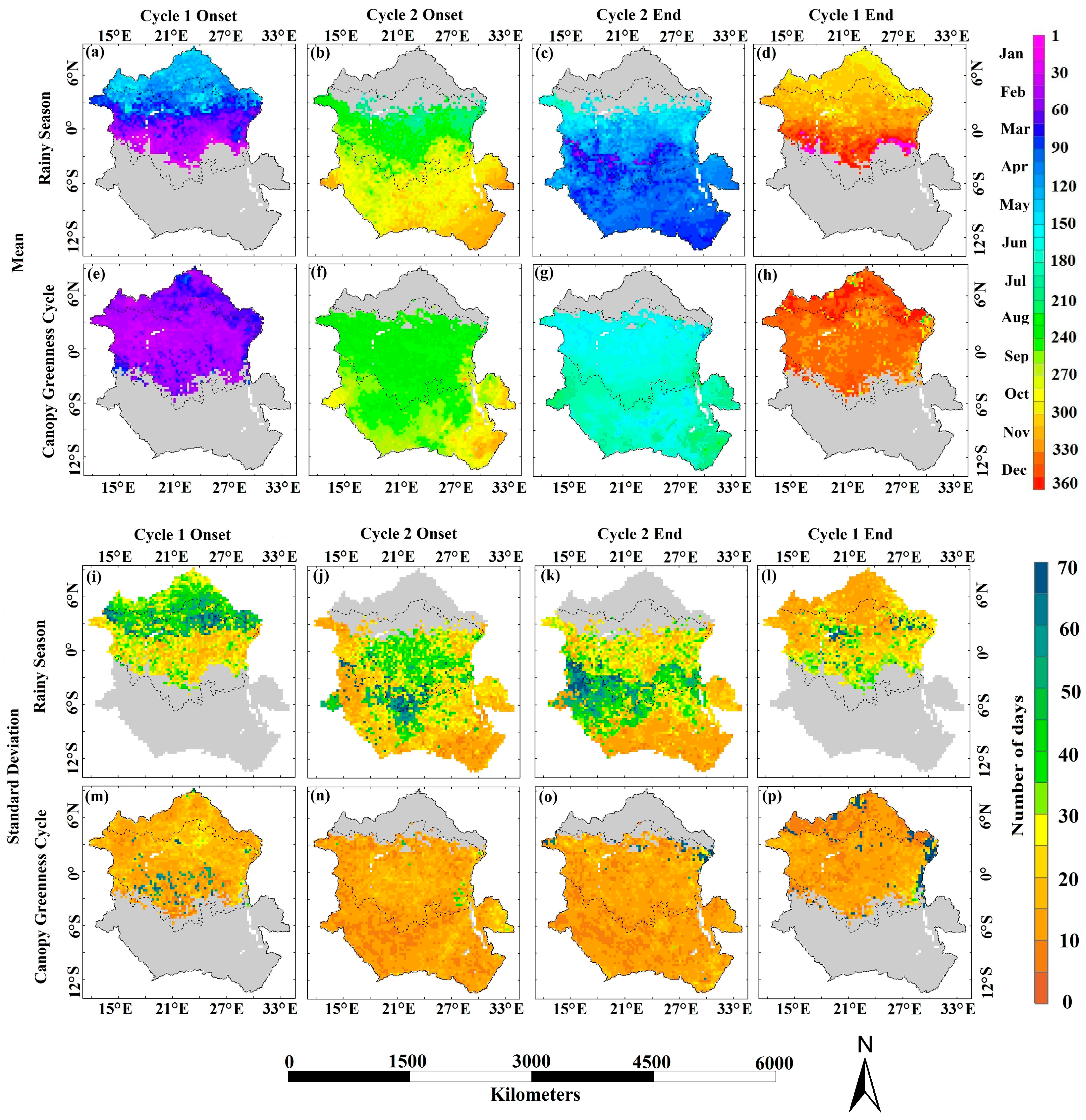
Figure 7.
Inter-comparison of cumulative distribution functions (CDF) of the timing differences between CGC and the rainy season, among the four land cover groups. Orange, dark red, green and dark green curves represent the CDF for grassland & shrubland, deciduous woodland & forest, deciduous forest & savanna mosaic and tropical rainforests, respectively. X-axis in (a–h) represents CGC onset lead time (i.e., CGC onset–ORS) whereas X-axis in (i–p) represents CGC end lag time (i.e., CGC end–ERS). For each land cover group, Y-axis specifies the proportion of grid cells with a timing difference, up to the difference specified on the X-axis.
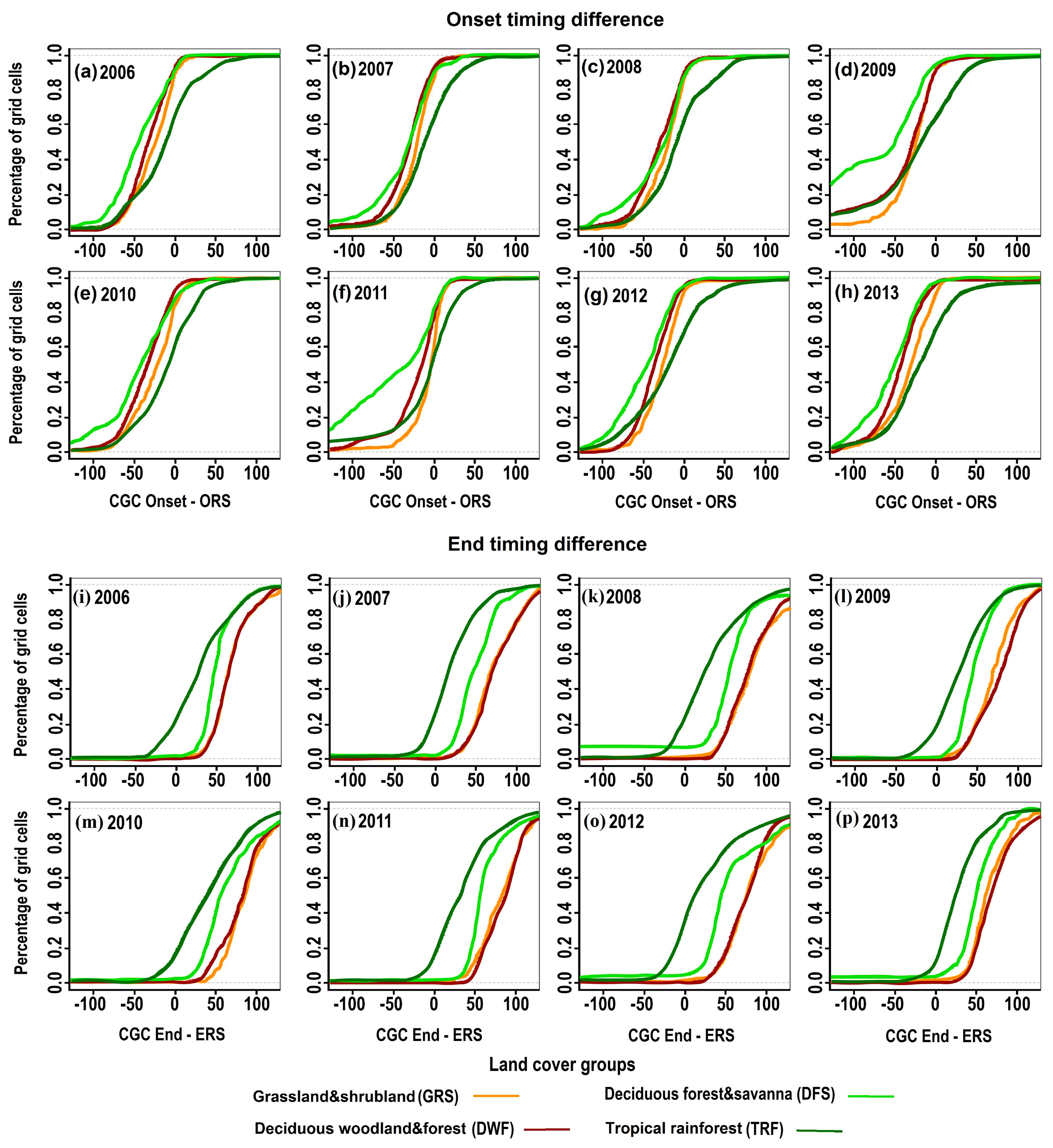
Figure 8.
Regression between spatial variation in ORS and CGC onset during 2006–2013 for grassland & shrubland (the top row), deciduous woodland (the middle row) and deciduous forest (the bottom row). X-axis represents ORS, whereas Y-axis represent CGC onset. The number of samples (N) used in each regression analysis is indicated at the upper left corner of a panel, whereas the R-squared value (R2) and residual standard error (RSE) are indicated at the lower right corner. The solid black lines represent the fitted regression lines, whereas the dashed black lines represent the 1:1 lines. Lighter shade indicates higher point density. The regressions shown in this figure are all significant at p < 0.001

© 2017 by the authors. Licensee MDPI, Basel, Switzerland. This article is an open access article distributed under the terms and conditions of the Creative Commons Attribution (CC BY) license (http://creativecommons.org/licenses/by/4.0/).
Share and Cite
MDPI and ACS Style
Yan, D.; Zhang, X.; Yu, Y.; Guo, W. Characterizing Land Cover Impacts on the Responses of Land Surface Phenology to the Rainy Season in the Congo Basin. Remote Sens. 2017, 9, 461. https://doi.org/10.3390/rs9050461
AMA Style
Yan D, Zhang X, Yu Y, Guo W. Characterizing Land Cover Impacts on the Responses of Land Surface Phenology to the Rainy Season in the Congo Basin. Remote Sensing. 2017; 9(5):461. https://doi.org/10.3390/rs9050461
Chicago/Turabian StyleYan, Dong, Xiaoyang Zhang, Yunyue Yu, and Wei Guo. 2017. "Characterizing Land Cover Impacts on the Responses of Land Surface Phenology to the Rainy Season in the Congo Basin" Remote Sensing 9, no. 5: 461. https://doi.org/10.3390/rs9050461
Note that from the first issue of 2016, this journal uses article numbers instead of page numbers. See further details here.