Optimizing the Processing of UAV-Based Thermal Imagery


1
Laboratory of Hydrology and Water Management (LHWM), Department of Forest and Water Management, Ghent University, Coupure Links 653—Bl. A, BE-9000 Ghent, Belgium
2
Ecosystem Dynamics Health and Resilience, Climate Change Cluster, University of Technology, Sydney (UTS), 745 Harris Street, Broadway NSW 2007, Australia
3
Laboratory of Plant Ecology, Department of Applied Ecology and Environmental Biology, Ghent University, Coupure Links 653—Bl. A, BE-9000 Ghent, Belgium
*
Author to whom correspondence should be addressed.
Remote Sens. 2017, 9(5), 476; https://doi.org/10.3390/rs9050476
Submission received: 3 March 2017
/
Revised: 5 May 2017
/
Accepted: 9 May 2017
/
Published: 12 May 2017
Abstract
:The current standard procedure for aligning thermal imagery with structure-from-motion (SfM) software uses GPS logger data for the initial image location. As input data, all thermal images of the flight are rescaled to cover the same dynamic scale range, but they are not corrected for changes in meteorological conditions during the flight. This standard procedure can give poor results, particularly in datasets with very low contrast between and within images or when mapping very complex 3D structures. To overcome this, three alignment procedures were introduced and tested: camera pre-calibration, correction of thermal imagery for small changes in air temperature, and improved estimation of the initial image position by making use of the alignment of RGB (visual) images. These improvements were tested and evaluated in an agricultural (low temperature contrast data) and an afforestation (complex 3D structure) dataset. In both datasets, the standard alignment procedure failed to align the images properly, either by resulting in point clouds with several gaps (images that were not aligned) or with unrealistic 3D structure. Using initial thermal camera positions derived from RGB image alignment significantly improved thermal image alignment in all datasets. Air temperature correction had a small yet positive impact on image alignment in the low-contrast agricultural dataset, but a minor effect in the afforestation area. The effect of camera calibration on the alignment was limited in both datasets. Still, in both datasets, the combination of all three procedures significantly improved the alignment, in terms of number of aligned images and of alignment quality.

1. Introduction
In recent years, the number of possible civil applications and the number of studies using UAVs (Unmanned Aerial Vehicles) or UAS (Unmanned Aerial Systems) has rapidly increased for a number of reasons. First, UAVs have become more affordable and reliable and their performance (flight execution, flight time, payload, range) has significantly increased. Second, the evolution in UAV development goes hand in hand with the miniaturisation of sensors. Potential imaging and non-imaging sensors include multispectral and hyperspectral spectrometers and cameras, LIDAR, microwave sensors, and thermal cameras (see e.g., Colomina and Molina [1] for a review). Third, processing software has been developed specifically for UAV data processing of both snapshot imaging and line scanning systems (such as most hyperspectral cameras).
Snapshot images are processed with Structure-from-Motion (SfM) photogrammetry [2]. SfM can be seen as an expansion of traditional stereoscopic photogrammetry in which matching features of a collection of overlapping images are automatically identified and used to calculate camera location and orientation. With this information, sparse and dense 3D point clouds are generated [3,4,5] that results in products such as a Digital Elevation Model (DEM) or an orthophoto.
In the last few years, SfM has been used extensively to process RGB (Red-Green-Blue) imagery and has become a reliable method for assessing the 3D structure of terrestrial systems, often matching the accuracies of much more expensive systems such as LIDAR. In geology, the technique has, for example, been used to monitor erosion rates [6] and landslide dynamics [7,8]. In agricultural and horticultural studies, it has proven to be a reliable tool for estimating crop [9,10] or tree [11] height. Similarly, the method has been embraced by forest engineers because it can provide high-quality forest inventory data, which is otherwise very time-consuming to assess from the ground [12,13,14,15,16]. In addition, SfM has become the standard tool for high-precision mapping (orthophoto generation) of agricultural and natural ecosystems e.g., [10,17,18].
SfM is not limited to processing standard RGB imagery. Most software packages have been extended and allow processing multi- and hyperspectral imagery as well [9,10,19]. Similarly, SfM can be used to process thermal images, which is the focus of this study.
As in other UAV disciplines, the number of applications of thermal imagery from UAVs in agricultural and ecological research has increased rapidly in recent years. In agriculture, UAV-based thermal remote sensing has been successfully applied for disease detection [20], high-throughput phenotyping in plant breeding [21], or for mapping drought stressed areas e.g., [22,23,24]. New developments also include the estimation of transpiration [25,26,27] or stomatal conductance [28]. In forestry and in ecological studies, the applications so far are less numerous, although the first studies indicate the usefulness of UAV-based thermal remote sensing in areas including fire detection [29], wildlife monitoring [30,31], assessing within-ecosystem variability in water availability [32], or in estimating plant growth and productivity [14].
Most of these applications rely on processing the thermal data with SfM for creating orthophotos. Turner et al. [33] provided a general framework for processing thermal imagery with UAV data, consisting of three steps:
- 1)
- Image pre-processing, which is the removal of blurry imagery and conversion of all images to 16-bit TIFF files in which all images have the same dynamic scale range, to ensure that a temperature value corresponds to the same digital number (DN) value in all images.
- 2)
- Image alignment, for which the initial estimations of the image position are derived from the on-board GPS log-file and the time stamp of each image.
- 3)
- Spatial image co-registration to RGB (or other) orthophotos is performed by manually adding ground control points (GCPs) with known position, either from real-time kinematic (RTK) GPS or from the processed RGB imagery.
Unfortunately, processing of thermal data with SfM does not always work flawlessly, and several studies have reported that SfM was not able to align thermal datasets properly [14,25,34]. In these cases, thermal maps could not be created or were created manually, by mosaicking separate images which were georeferenced manually using GCPs. These issues with thermal datasets are a consequence of the limited information contained by thermal images compared to RGB images, rendering the detection of common features needed for the bundle adjustment problematic. Indeed, in contrast to RGB or multispectral images, almost all thermal cameras for UAVs have one single band (one thermal measurement per pixel in the entire 8–12 μm region). In addition, the image resolution of the thermal images is very low. Whereas even consumer-grade RGB cameras have a resolution of 12 MP or higher, most UAV thermal cameras have a resolution of 0.077 (320 × 240 pixels) to 0.33 MP (640 × 512 pixels). This implies that small features that stand out in (for instance) RGB are less or not visible in the thermal imagery. In the studies with problematic thermal image alignment mentioned above, alignment was not possible because of the low contrast in surface temperature between and within the images (very homogeneous canopy). In addition, from our personal experience, we noticed that alignment is often problematic in ecosystems with complex structures, such as forests.
There are, however, a few ways to overcome this alignment issue. One option is to adjust the flight mission and to increase the vertical (lower flight speed) and horizontal overlap (flight lines closer to each other). However, this comes at the obvious cost of the reduction of the area that can be overflown in one flight and, moreover, it is not guaranteed that this will solve all alignment issues. Alternatively, some thermal cameras have an incorporated RGB or even multispectral camera, with similar or higher resolution, taking images simultaneously. In this case, the images can be processed as multispectral images and can be aligned based on the RGB information. Otherwise, if an RGB and thermal camera have fixed positions relative to each other and are triggered to take images at the same moment, the RGB and thermal data can be co-registered based on a fixed transformation of one image pair [35], and thermal data can also be aligned along with and based on the RGB images. In most applications, however, thermal cameras are not equipped with an integrated RGB camera, or the simultaneous triggering of the RGB and thermal camera is difficult or practically not feasible. Yahyanejad and Rinner [36] developed an algorithm to co-register RGB and thermal images. However, their algorithm was so far only tested on datasets with high contrasts in both the RGB and the thermal images, and moreover, their algorithm is not (yet) publicly available.
There is another issue related to the processing of UAV-based thermal imagery that has so far received little attention. Flights regularly take up to 20 min or longer. When larger areas need to be covered, several flights are required, and it is not uncommon that 45 min or more have passed between the first and final image of the dataset. Even if measurement conditions are ideal—low wind, open skies—the air temperature will likely have changed during this period. This has a large impact on the canopy surface temperature, which is the sum of air temperature and a complex function of vegetation features, wind speed, available energy, and transpiration [37,38].
In this study, we investigated methods to optimize UAV-based thermal image processing. We propose several improvements of the basic framework introduced by Turner et al. [33], which allows aligning and processing of complex and more challenging datasets to obtaining thermal orthophotos corrected for changing conditions over flight measurements. This improvement makes use of the information from a RGB (or NIR) camera on board the UAV, since in the large majority of the flights, these are taken along to be able to interpret the thermal information. The improvements are illustrated and tested using two datasets, for which the standard processing framework gave unreliable results. The first dataset is a very homogeneous agricultural field, while the second dataset, an afforestation site, has a complex canopy structure.
2. Materials and Methods
2.1. Background on the Influence of Meteorological Conditions on Thermal Data Collection and Processing
When working with thermal infrared data, there are several ways in which meteorological conditions influence the thermal signals and need to be corrected for.
First, meteorological conditions can exert an indirect effect on the observed temperatures. Thermal cameras on UAVs typically have uncooled microbolometer sensors with the thermal signal being highly influenced by the temperature of the sensor, body and lens. Even though this is (at least partially) corrected for in radiometric cameras, abrupt changes in sensor temperature (e.g., when moving from shaded to unshaded conditions) can cause errors in the observed temperature. Particularly lightweight thermal cameras can be more sensitive to these sensor temperature fluctuations and might require additional temperature corrections. This can for instance be done by taking images of wet or dry reference panels/surfaces with known temperatures (at least) before and after the flights. The temperature of these reference panels needs to be measured directly and accurately (e.g., with contact thermocouples) and these measurements can then be used to compensate for changes in sensor temperature. In this study, we used a relatively sturdy thermal camera with an excellent sensor temperature correction (temperature accuracy ±2%, see further). As we have not noticed a drift in Ts in these flights or even in more extreme conditions, no contact thermocouple measurements of references surfaces were taken.
The second way in which meteorological conditions influence thermal measurements is by attenuation of the thermal radiance by the atmosphere. The thermal sensor registers an at-sensor radiance, Lat-sensor [W m−2] for each pixel. This is determined by the surface radiance (Lsurf, [W m−2]) and by its attenuation by the atmosphere [39]:
where τ is the atmospheric transmittance (dimensionless; value between 0 and 1) and Latm [W m−2] is the upwelling thermal radiation originating from the particles in the atmosphere. Both τ and Latm are mainly a function of the atmospheric water content and the distance between the sensor and the object. Usually, Lat-sensor is automatically converted into Lsurf by the thermal camera software based on input from the user of the distance between the sensor and the surface, relative humidity and temperature. Alternatively, τ and Latm can be calculated from an atmospheric propagation model such as MODTRAN e.g., [40]. In this article, we used the input from the meteorological station and flight height (see further) as input for the thermal camera software (see further).
From Lsurf, the surface brightness temperature Tbr [K] can be calculated using Stefan Boltzmann’s law (L = σ·Tbr4, with σ = 5.67 × 10⁻⁸ W m−2 K−4 the Stefan Boltzmann constant):
The brightness temperature of an object is composed of two signals. The first signal is the thermal emission by the object, reflected by the surface temperature Ts [K]: this is the signal of interest in thermal remote sensing, as it is reflecting the energy balance of the object. The second signal composing Tbr is the reflectance of the incoming thermal radiation by the object, which is represented by the background temperature (Tbg, [K]), or the temperature corresponding to the incoming long-wave radiation. Ts can be estimated from Tbr and Tbg as [38],
with ε the emissivity of the object. From Equation (3), it is clear that a calculation of Ts from Tbr requires the additional measurement or estimation of Tbg and ε. Ways to measure/estimate Tbg are described by Maes and Steppe [38]. In this study, we used the common method of measuring the temperature of blotted aluminium foil. The emissivity, however, is more difficult to estimate, and small errors in its estimate can lead to relatively large errors in the estimate of Ts [38]. Dense plant canopies have an emissivity between 0.98 and 0.99 [41,42]; in this study, we used a value of 0.985. For open canopies, the NDVI method can be used [42], provided NDVI data are available.
Finally, meteorological conditions directly determine Ts, as Ts can be expressed as [38],
with Ta the air temperature [K or °C], Rn the net radiation [W m−2], G the ground heat flux [W m−2], VPD the vapour pressure deficit [Pa], s the slope of the curve relating temperature to saturated vapour pressure [Pa K−1], the air density [kg m−3], cp the specific heat of air [J kg−1 K−1], the psychrometric constant [Pa K−1], raH the resistance of heat transfer and rv the resistance of water transfer (both [s m−1]), which for vegetations is given as rv = raH + rc, with rc canopy resistance of water transfer. From Equation (4), it is obvious that an increase in air temperature will directly result in a similar increase in Ts. Furthermore, increasing net radiation or vapour pressure deficit will also increase Ts, although this effect is additionally controlled by adjustments by the vegetation in rc.
From Equation (4), it is clear that changes in meteorological conditions during the flight will influence Ts. Without correction of this noise, interpretation of the orthophoto is hampered, as colder or warmer areas can both indicate higher or lower transpiration, or lower or higher air temperature, radiation, etc. In Section 2.3, we introduce a way to correct for fluctuations in air temperature.
2.2. Flights and System Set-Up
2.2.1. Flight System
The UAV was a Vulcan hexacopter (Vulcan UAV, Gloucestershire, UK), equipped with an A2 flight control system (DJI, Shenzhen, China). Maximum flight time is approximately 20 min, with a maximum range of 2 km and a maximum take-off weight of 10 kg.
Rather than using the automatic waypoint generation included in Ground Station 4.0.11 (DJI, Shenzhen, China), the software used for communicating with the UAV, a Matlab script (Matlab R2015b; Mathworks Inc., Natic, MA, USA), was developed to generate the waypoint path. The waypoint path is exported as an AWM file, readable in Ground Station 4.0.11, and is sent to the UAV using the wireless 2.4 GHz Data Link module. Using the script offers the advantage that waypoints are not only restricted to the corners, but can also be positioned along the flight line, so that the UAV sticks to the path. Furthermore, the width between parallel lines can be accurately defined, guaranteeing sufficient horizontal overlap.
The UAV was equipped with a separate GPS logger system (Aaronia, AG, Strickscheid, Germany), logging with a frequency of 10 s−1, with an RGB and thermal camera mounted on a 2D AV2000 gimbal (PhotoHigher, Wellington, New Zealand), and programmed to maintain pitch and roll close to 0° during the flights.
The RGB camera was a 12MP Canon S110 (Canon, Tokyo, Japan). The focal length during the flights was set to 5.2 mm (24 mm equivalent), which corresponds with a field of view of 74° × 53° and a pixel resolution of 1.9 cm at 50 m flight height. The camera is programmed with CHDK to log continuously every 1.1 s and operated in Tv-mode (shutter speed priority). The camera automatically adjusted the camera aperture (f-number) based on the first shot and maintained the same image settings during the entire flight.
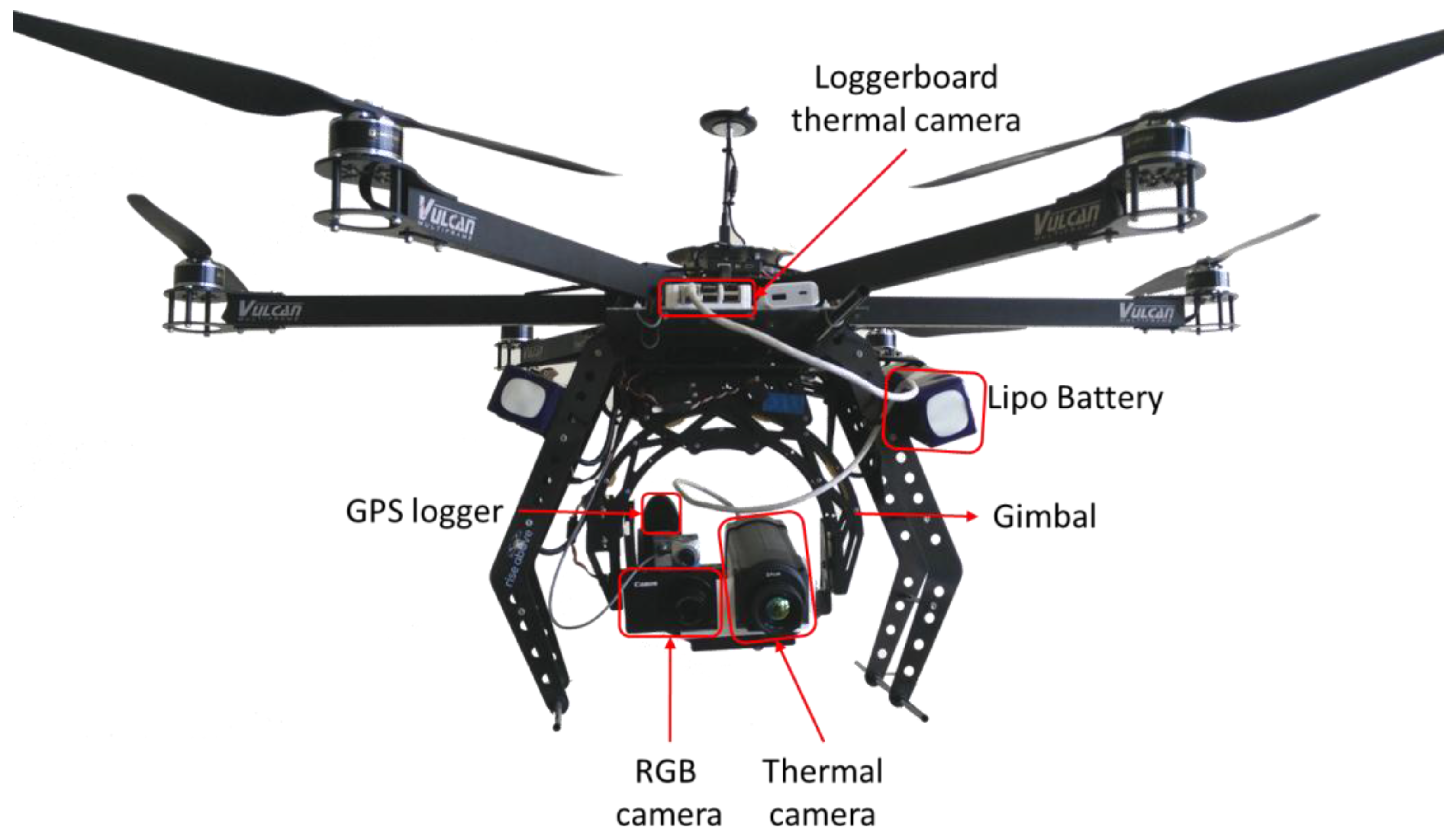
The thermal camera is a Flir SC305 (FLIR Systems, Inc., Wilsonville, OR, USA) with a resolution of 320 × 240 pixels, a thermal accuracy of 2 °C, and a thermal sensitivity of 0.05 °C. It was equipped with a 10 mm lens, offering a field of view of 45° × 34°. At 50 m altitude, the pixel resolution (central pixel) is 12.8 cm and each thermal image covers an area of 41.4 by 30.6 m. The camera is controlled through a Python script on a Raspberry Pi development board onboard the UAV and logs continuously every 0.8–1.1 s, although occasionally the interval between two consecutive photos was larger because of camera recalibration (gap of about 4 s). The thermal and RGB cameras were not synchronized. All images are stored as 8-bit lossless JPEGs. A schematic overview of the UAV, sensors, and components used in this study is given in Figure 1.
2.2.2. Agricultural Dataset
In this study, two datasets were analysed. The first dataset is a field of 8.7 ha, situated in Huldenberg (50°48′ N, 4°34′ E) in the loamy region of Flanders, Belgium. In 2016, it was cultivated with beets (Beta vulgaris L.), which had formed a dense crop of circa 0.5 m high by the time of the flights. The field was planted with two different cultivars of beet: the Northern part of the field was planted with Bambou, the Southern part with Gondola. The Gondola cultivar grows more slowly than the Bambou cultivar at the start of the growing season to become greener and typically has a larger photosynthetic activity towards the end of the growing season, when the flights were performed.
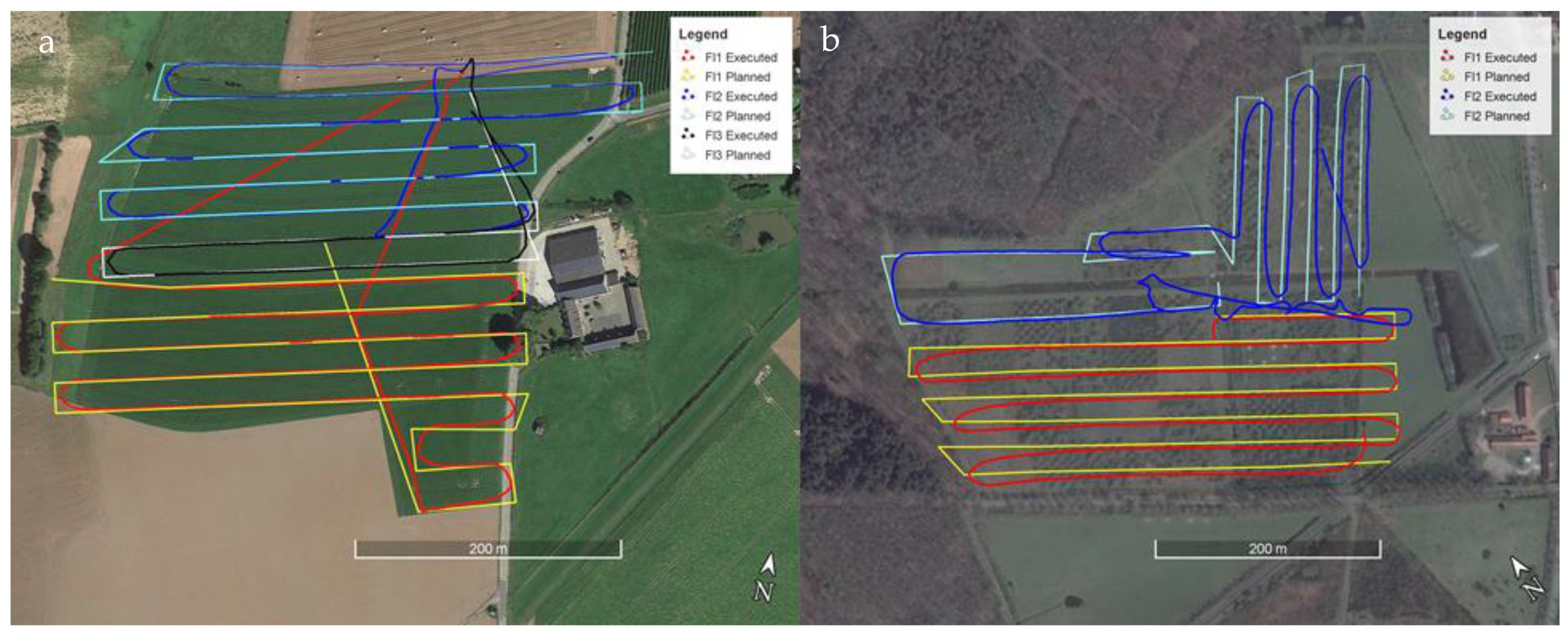
To cover the entire field, three flights were performed in cloud-free conditions on 25th August, 2016 (See Figure 2a), between 13:11 and 13:57 local time (Table 1). The flight altitude was set to 50 m and flight speed was 4 m s−1. The flight lines were 350 m in length with a distance of 20 m between each parallel line (Figure 2a). This resulted in a vertical overlap of 86% and a horizontal overlap of 52%. A microclimatic station (CR6 data logger, Campbell Scientific Inc., Logan, UT, USA) was installed next to the beet field, logging air temperature (MCP9700, Microchip Technologies Inc., Chandler, AR, USA), relative humidity (HIH4000, Honeywell International Inc., Morris Plains, NJ, USA), wind speed (A100R, Vector Instruments, Rhyl, UK) and net radiation (Q7.1, REBS, Seattle, WA, USA) every 10 s. An overview of the microclimatic conditions during the flight is given in Table 1.
Eight reference panels were laid out on the edges of the field. These reference panels were each 60 by 60 cm and were wooden panels painted with extra matt grey paint. They were visible in the RGB and thermal images. To measure Tbr, one panel was wrapped with crumpled aluminium foil and was positioned close to the take-off and landing position. At the start and at the end of each flight, the UAV was steered to hover directly above this reference panel.
2.2.3. Afforestation Dataset
The second dataset was collected above the Forbio site in Zedelgem, Flanders (51°9′ N; 3°07′ E), on 24 August 2016. This is an experimental afforestation site on relatively dry sandy to moderately wet loamy sand soil. The site belongs to the TreeDiv network [43] and consists of 42 blocks, each of 42 × 42 m, in which trees of five different species were planted in 2009–2010 within a 1.5 × 1.5 m planting grid. A detailed description of the experimental set-up can be found in Verheyen et al. [44] and Van de Peer et al. [45]. In total, the site covers about 11.4 ha. Two flights were needed to cover this area completely. The first flight had six parallel lines of 420 m long and with a distance of 21 m in between. The second flight covered a less regular shape, and consisted of six shorter parallel lines in perpendicular lines, followed by two more long lines parallel to the lines of the first flight (Figure 2b). The flight height was again 50 m and the flight speed 4 m s−1, so the vertical and horizontal overlap of the thermal images were 86% and 49%.
Similar to the agricultural dataset, eight reference panels were positioned across the site, with an aluminium reference panel close to the take-off and landing area for assessment of Tbr. The same microclimatic station was installed at the site and logged throughout the flights. Flight details can be found in Table 1.
2.3. Data Processing
2.3.1. Suggested Improvements
a. Camera Pre-Calibration
Lens distortion is a radially dependent geometric shift or deviation from the rectilinear projection [46]. As SfM is very sensitive to distortion, camera calibration is a crucial pre-processing step [4,47]. Some software packages, including the Agisoft PhotoScan Professional (Agisoft LLC, St Petersburg, Russia) software used in this study, automatically perform a camera calibration using the Brown-Conrady distortion model (on-the-job self-calibration). Unfortunately, this self-calibration is not performed on low-resolution thermal imagery.
The parameters of the Brown-Conrady distortion model can be obtained separately, for instance with Agisoft Lens (Agisoft LLC, St Petersburg, Russia), software, which is part of the Agisoft PhotoScan product (pre-calibration). This uses multiple images of a calibration grid, which is usually displayed on a flat panel screen and then imaged with the camera [46]. As this does not work with a thermal camera, the grid was printed on an A3 sheet of paper, which was fixed on a rigid wooden frame. This was placed horizontally under a tungsten light in a growth chamber to create enough contrast between the white and black parts of the paper. The thermal images of this grid then served to calculate the distortion parameters in Agisoft Lens and pre-calibrate the camera. The parameters of the calibration are given in Table 2.
b. Temperature Correction
As explained in Section 2.1 Equation (4), Ts is closely coupled to air temperature Ta. Hence, as Ta changes during the flight or over consecutive flights, so will Ts (Figure 3). Therefore, we applied following correction for Ta:
with Ts_c the corrected Ts, Ta the air temperature at the moment of image capture and Ta_mean the mean air temperature during the three (agricultural) or two (afforestation dataset) flights. Air temperature (Ta) was obtained from the logged air temperature measurements and the timestamp of the thermal image using a linear spline function. The corrected surface temperature (Ts_c) images were calculated in Matlab R2015b and converted to 16 bit TIFF images.
Ts_c = Ts − Ta + Ta_mean
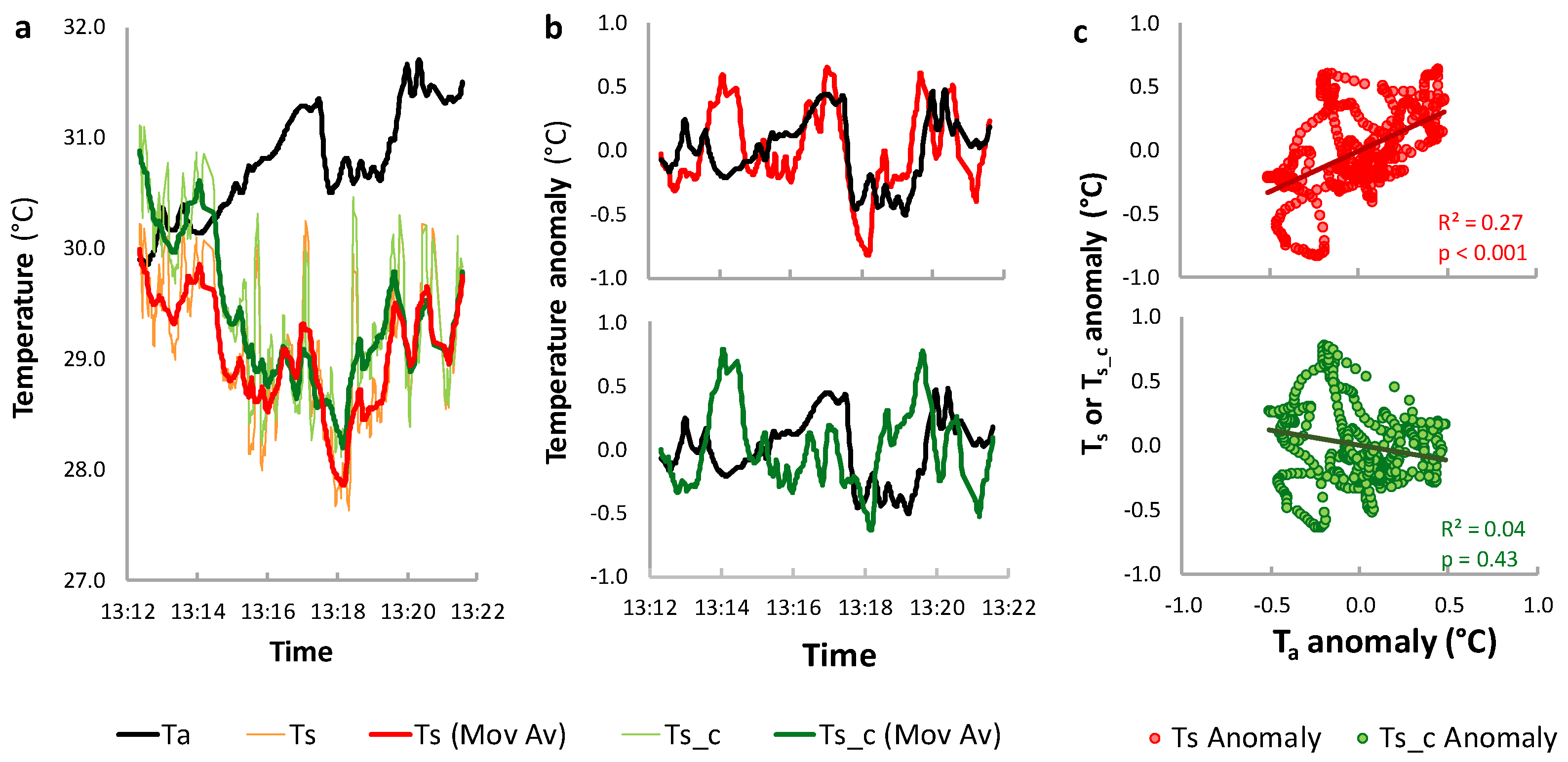
The close correlation between Ta and Ts and the effect of the temperature correction Ts_c is shown in Figure 3 for the first flight of the agricultural dataset. Figure 3a shows Ta, Ts and Ts_c as well as the moving averages (of 20 images, about 20 s) of Ts and Ts_c as a function of time. Ta seems only weekly coupled with the moving average of Ts, as Ts first decreases at the start of the flight, whereas Ta is then increasing. However, the sudden drop in Ta at about 13:17 has a clear impact impact on Ts, as does the abrupt increases in Ta at 13:19. The anomalies of the moving averages of Ts and Ts_c and of Ta are plotted as a function of time in Figure 3b. The anomalies were calculated as (Tobs − Texp), with Tobs the observed and Texp the expected Ta, Ts or Ts_c. Texp was calculated as a function of the time from a 2nd order polynomial function fitted through Ta (R2 = 0.68) and through the moving averages of Ts (R2 = 0.54) and Ts_c (R2 = 0.75). Plotting the anomalies as a function of time confirms the close connection between the abrupt increases or decreases of Ta on Ts (Figure 3b, upper part), which is nearly completely corrected for when using Ts_c (Figure 3b, bottom part). In Figure 3c, scatter plots of the anomalies of Ta vs. Ts and of the anomalies of Ta vs. Ts_c are drawn, revealing that the anomalies of Ta vs. Ts are significantly correlated, whereas the anomalies of Ta vs. Ts_c are not (Figure 3c).
c. Improved Estimation of Image Position
In general, the better the initial estimate of the image position, the better the image alignment will be. In the standard approach, the image position is derived from the on-board GPS log-file and the time stamp of each image. In our proposed alternative approach, we first optimize the alignment of the RGB imagery. This includes the image alignment of the RGB images, the addition of GCPs and the optimization (in the Agisoft software) of the image positions (Section 2.3.2). We then used the optimized RGB image positions (latitude, longitude, altitude, pitch, yaw, and roll), and estimated those of the thermal images based on the time stamp of the RGB and thermal images using a linear spline function. In addition, we also ran the model without using any information of the image position.
2.3.2. Data Processing
a. Data Processing of RGB Imagery
After all data were collected, the visual images were inspected and blurred images were removed. In both datasets, less than 1% of images were removed. Based on the timestamp of each image and on the GPS log, a Matlab R2015b script was developed to estimate the latitude, longitude, and altitude of the RGB images using a linear spline function. In the afforestation dataset, there was a problem with the GPS logger and no GPS data were available. Instead, we derived the estimated latitude, longitude and altitude of each RGB image from the planned waypoint route. This was done by first identifying the images taken at the start and at the end of each flight lines. The target position of the waypoint was then attributed to these images and the position of all other images was estimated based on the time stamp of this image and those of the images at the start and the end of the flight line.
Agisoft PhotoScan Professional version 1.2.6 was used to process the visual data. The RGB images of the two (afforestation) and three (agricultural) flights were aligned (selecting highest accuracy and reference pair selection as settings). In the agricultural dataset, 1033 of 1044 images were aligned. Next, 33 GCPs were identified and added, of which 17 GCPs had known latitude, longitude, and altitude coordinates. As no GPS-RTK measurements were available, these coordinates were identified from high-resolution aerial imagery available from Google Earth, from which the altitude estimates were also taken. In the afforestation dataset, 1027 of the 1031 images were aligned and 31 GCPs (of which 16 with known coordinates) were used to co-register and georeference the images. Finally, the image positions were optimized and exported, a 3D mesh was calculated and a visual orthophoto generated and exported.
b. Thermal Data Pre-Processing
All thermal data were originally stored as lossless 8-bit JPEG files and blurred images were removed. In the agricultural dataset, 10% of the images (148 of 1488 images) were removed, in the afforestation dataset, this was 17.3% of the images (219 of 1264 images). The remaining images were opened in ThermaCam Researcher Pro 2.10 (FLIR Systems, Inc., Wilsonville, OR, USA), embedded in Excel 2010 (Microsoft, Redmont, WA, USA). Using the microclimatic conditions (RH, Ta) and the target height and setting the emissivity to 1, the at-sensor radiance was converted to Tbr Equations (1) and (2), as described by Maes et al. [48]. The background temperature (Tbg) before and after the flight was derived from the temperature of the aluminium foil-covered reference target and was averaged and a suited temperature range (maximum and minimum temperature) was defined.
All images were opened in Matlab R2015b and were converted to surface temperature Equation (3). Emissivity was set at 0.985 for all flights and images were saved as 16 bit TIFF files. In addition, the Ts_c images were calculated Equation (4) and also saved as 16 bit TIFF files. Using the timestamp of the thermal image and a linear spline function, the GPS-based image position (latitude, longitude, altitude) was estimated based on the GPS logfile (agricultural dataset) and the planned waypoint flight (afforestation dataset), similar as was done for the visual dataset. In addition, based on the exported image position of the visual images, the improved image position (latitude, longitude, altitude, yaw, pitch and roll) of each thermal image was calculated, again using a linear spline function.
c. Alignment Procedures
For both datasets, we tested the calibration methods (two levels: with and without calibration), the temperature correction (two levels: with and without temperature correction) and the influence of the initial estimate of the image position (three levels: without initial estimate, with input from GPS logger, with input from RGB image position), resulting in 12 different processing treatments.
All alignment tests were performed with Agisoft PhotoScan Professional version 1.2.6. For each scenario, the correct TIFF files (Ts or Ts_c files) were imported. The calibration file was imported if required and the images were aligned. The highest accuracy, reference pair selection (generic pair selection when no initial GPS position was used as input) and standard key point limit of 20,000 and tie point limit of 1000 were used as alignment settings.
Often, not all images were aligned after a first alignment procedure. However, PhotoScan allows selecting non-aligned images together with overlapping aligned images and re-aligning the selected images. If this re-alignment resulted in meaningful, realistic alignments, they were maintained.
d. Comparison of Different Alignment Approaches
To compare the different alignment approaches, we first looked at the number of aligned images and at the number of points in the point cloud. However, we also looked at the quality of the alignment. For this, we checked for the presence of the following:
- A bowl effect, where there is a systematic deviation in image alignment, causing a flat surface to become bent in the X- and Y-direction the shape of a bowl;
- Alignment gaps, defined as areas where several consecutive images were not aligned, leading to areas without any points;
- Images that are clearly not aligned correctly, which can be detected by clear deviations in the point cloud.
e. Further Processing
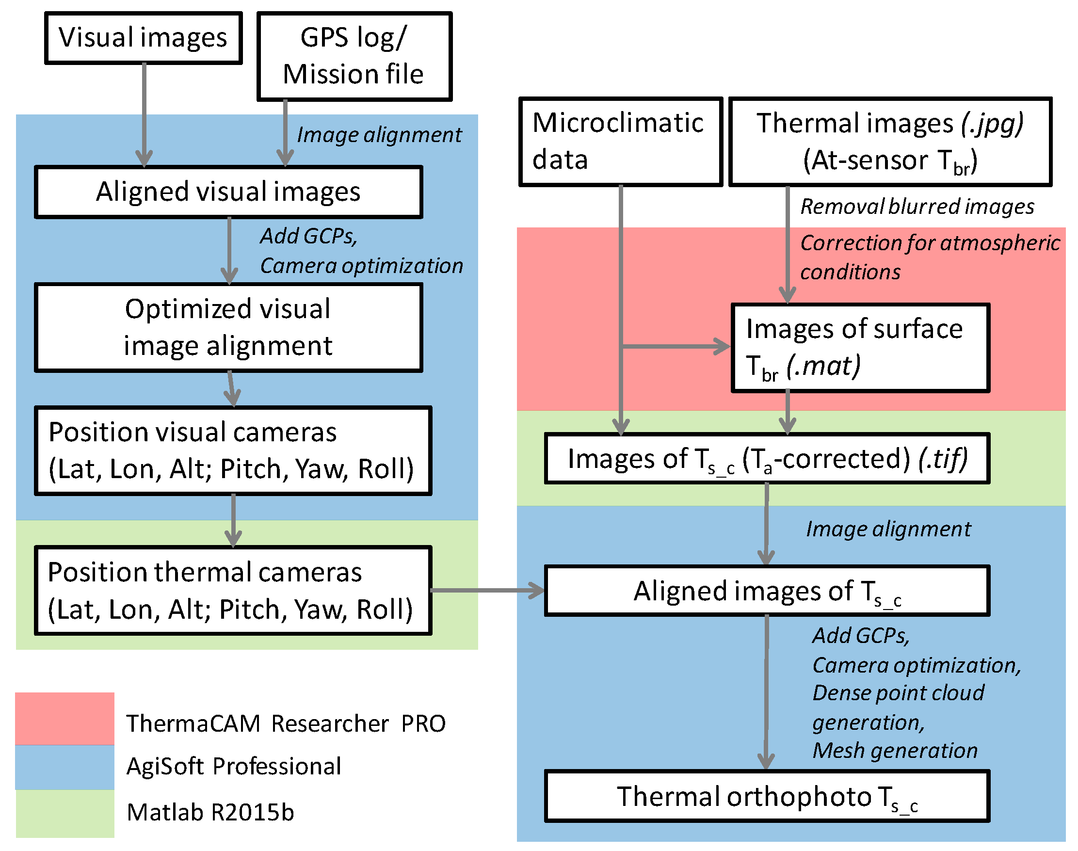
For each dataset, an orthophoto was created using the imagery of the best performing alignment approach. The same GCPs as for the RGB image alignment were used, the dense point cloud was calculated using the highest density setting, a 3D mesh was created based on which the orthophoto was finally created and exported. An overview of all thermal image processing steps is provided in Figure 4.
3. Results
3.1. Agricultural Dataset
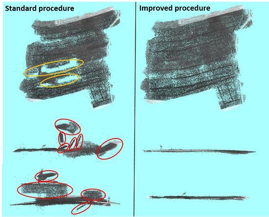
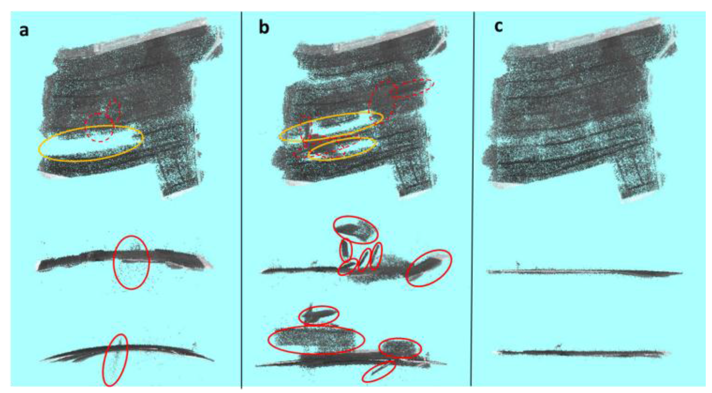
An overview of the resulting alignment of the agricultural dataset is given in Table 3. The method used for the initial thermal image position had clearly the strongest effect on image alignment. When no initial thermal image position was used, a larger number of images was not aligned, fewer points were aligned, a bowl effect was clearly visible, and large gaps in the dataset were present (Figure 5a). When the GPS-log was used as original image positions estimate, the bowl effect was no longer present (except for one alignment scenario), but several sections were wrongfully aligned (Figure 5b and Table 3). The best alignment results were obtained when the initial thermal image positions were based on the estimated positions of the RGB images during the flight (Figure 5c). Replacing Ts with Ts_c had a small, yet clearly positive effect on the alignment, slightly increasing the percentage of aligned images and the number of aligned points (Table 3).
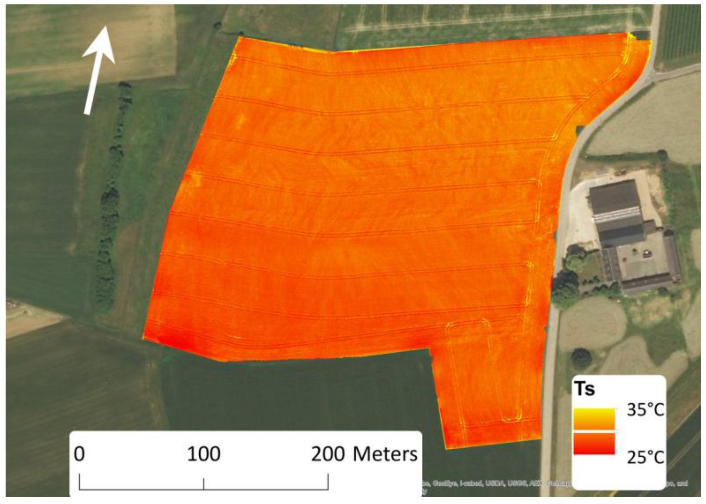
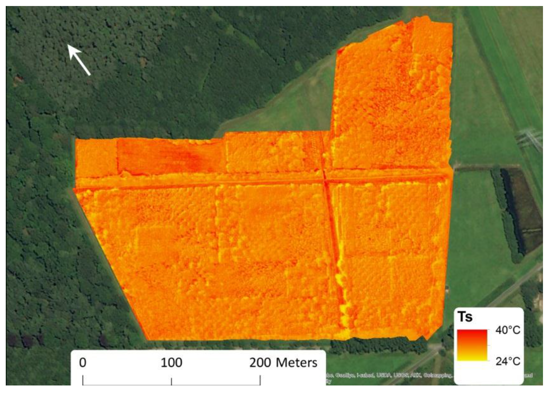
In contrast, the effect of the camera pre-calibration overall was negative, with one exception: when Ts_c was used as variable in combination with the RGB-based initial image position estimate and the use of the camera calibration file, all sections were correctly aligned, without any gaps, and with a very high number of images and number of points that were aligned (Table 3). Hence, this can be regarded as the best performing model. The thermal map resulting from this optimized model is shown in Figure 6. Note that the Southern part of the field, which was planted with the Gondola variety, is slightly cooler, in agreement with the expected higher photosynthetic activitiy at this time of year.
3.2. Afforestation Dataset
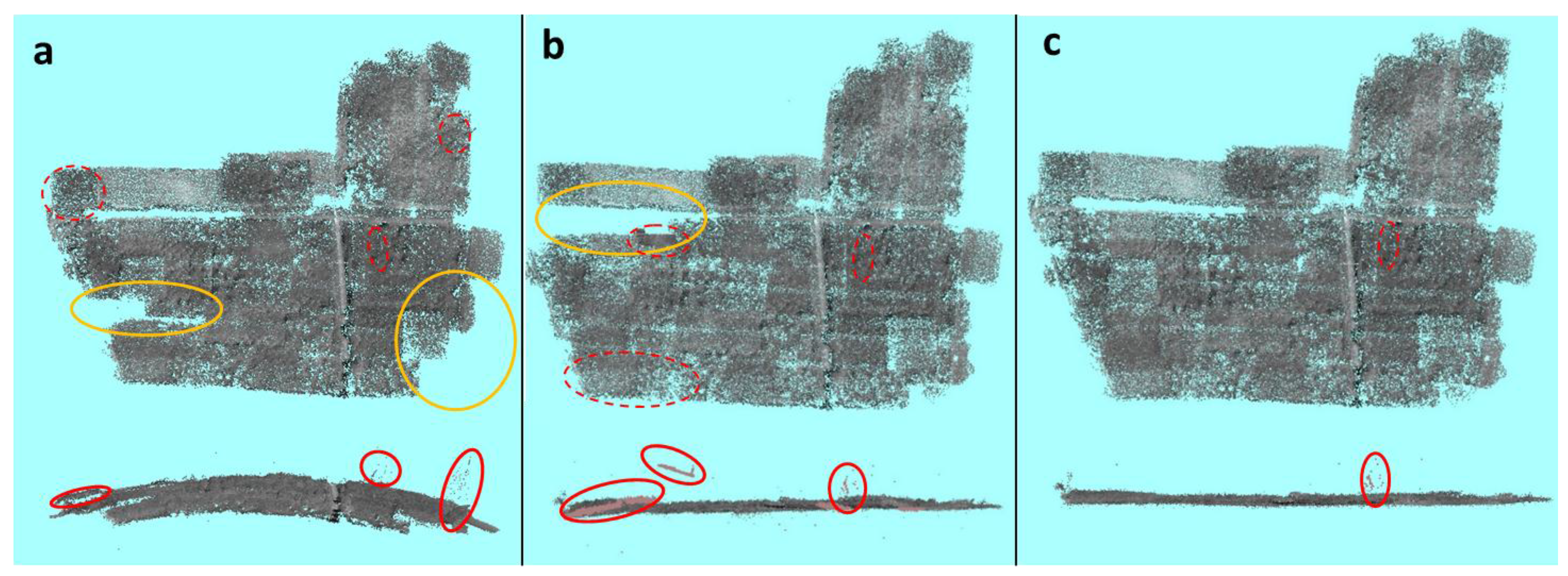
An overview of the resulting alignment of the afforestation dataset is given in Table 4. The number of images aligned and the number of points are clearly lower for the alignments without any initial image position input. As a consequence, these alignment methods also had most gaps and had a few sections that were not aligned correctly (Figure 7a). The two methods with information on image position had nearly all images aligned and had a comparably high number of aligned points. Although the alignments with the mission file-based GPS positions overall had a slightly higher number of aligned points and slightly higher number of images aligned, there were several sections not aligned properly. This was not the case for the alignments using RGB-based image positions as initial input (Figure 7b,c).
In general, the effect of using Ts_c improved the alignment although this effect was very limited. Camera calibration had a very small effect and only improved the alignment where no GPS input was given and when the GPS input was based on the RGB alignment. The thermal map using the RGB-based image position is shown in Figure 8.
4. Discussion
It is clear from the datasets that the use of image positions of the RGB imagery for initial estimates of thermal image positions greatly improved thermal image alignment, both in terms of number of aligned images and in quality of the alignment (absence of bowl effect; fewest misaligned areas; absence of alignment gaps). With this method, on all flights, the few non-aligned thermal images were those taken when the UAV was turning to move to the next waypoint. With the DJI A2 flight control system, the UAV turns quite abruptly at the end of each flight line. At these instances, the spline function from the yaw position of the RGB images, used to estimate the yaw of the thermal image, can have a relatively large error leading to misalignments. In addition, these images are often less sharp, particularly in the corners, due to the sudden turns.
The most important reason for the superior performance of the RGB imagery-based image positions is probably the availability of the pitch-yaw-roll information. Similar alignment results could be obtained when using a GPS unit in combination with an inertial measurement unit (IMU), monitoring pitch, yaw, and roll, mounted on the gimbal. Small and low-cost IMUs have become available for this purpose. The benefit of using a GPS + IMU unit is that it does not rely on the RGB images and thus removes the need to first align the RGB imagery, thus speeding up the process considerably, which can be very relevant in case rapid thermal maps need to be constructed. Aligning the RGB images, manually adding GCPs, and optimizing the images can take several hours, with the computing time, depending on the settings (alignment precision), the computer specifications, and the number of images used. On the other hand, IMUs can be sensitive to magnetic errors when mounted on drones [49]—in fact, the GPS system used in this study was equipped with an IMU as well, but the pitch-yaw-roll readings were unusable because of magnetic interference. Proper shielding of the IMU unit can prevent this. It needs to be confirmed if the precision of the pitch-yaw-roll log from cheaper IMUs can match those of the image alignment.
On the other hand, an advantage of using the RGB imagery-based image positions is that it facilitates co-registration of visual and thermal images, required for further data processing as well as for data interpretation. Moreover, the afforestation dataset analysis demonstrated that GPS measurements are not required to come to high-quality thermal alignment, if the optimized method (RGB images as initial image position) is used. One possible disadvantage of the method is that the UAV needs to be equipped with an RGB camera (or IMU). This is the case in most applications, but else can increase the payload and reduce the flight time.
The temperature correction had a different effect in both datasets. In the agricultural dataset, temperature correction had a small but clearly positive effect on image alignment. This dataset is characterized by low contrast within and between the images. If no correction is made for the influence of air temperature on surface temperature, small, artificial differences in Ts between the images can hamper image alignment. In the afforestation dataset, on the other hand, temperature correction had little effect on image alignment. This is in line with the expectations. The alignment of this dataset is problematic because of the complex 3D structure of the vegetation—this is not solved by temperature correction.
We want to emphasize that temperature correction not only has an effect on the image alignment but also removes the influence of Ta on Ts. In our flights, maximal air temperature differences during the flights were as much as 1.9 and 1.7 °C for the agricultural and afforestation datasets, respectively, and has large consequences on Ts (Figure 2). This can be corrected for using Ts_c. As explained in Section 2.1, it can be useful, particularly when working with lightweight thermal cameras, to additionally lay out reference surfaces, whose temperature is monitored continuously, e.g., with contact thermocouples, to correct for temperature fluctuations of the temperature of the camera sensor, lens and body
Adding the camera pre-calibration did not significantly improve the photogrammetric alignment, in contrast with findings by Harwin et al. [47] for visual images. In some trials, pre-calibration even seemed to yield worse alignment results (e.g., see Table 3 and Table 4). Still, although the contribution was limited, the best performing methods were those who also incorporated calibration, next to optimized GPS positioning and temperature correction.
5. Conclusions
In this study, we provide an improved framework for aligning and further processing UAV-based thermal imagery. Three improvements were introduced: camera pre-calibration, correction of thermal imagery for small changes in air temperature, and improved image position estimation by making use of RGB camera alignment. These improvements were tested in two datasets that are problematic for thermal image processing: a dataset over a beet field with very low temperature contrasts within the field, and a dataset over an experimental afforestation area, with very complex 3D structure.
In both datasets, the standard alignment procedure failed to align the images properly. Using RGB image-based image positions significantly improved image alignment in all datasets. Air temperature correction had a small yet positive impact on image alignment in the low-contrast agricultural dataset, but a minor effect in the afforestation area. The effect of camera calibration on image alignment was limited in both datasets, yet the best alignment, in terms of numbers of images aligned and of alignment quality, was obtained when the three improvements were combined.
Acknowledgments
This study was funded by the Marie Curie IOF project (PIOF-GA-2012-331934) within the 7th European Community Framework Programme. The thermal camera was funded by the Flemish Agency for Innovation by Science and Technology (IWT) on the Agricultural Research project TipRelet. The flights over the agricultural site were performed in the framework of and supported by the Bayer Forward Farming endowed chair at the Faculty of Bioscience Engineering, Ghent University. We would like to thank Kris Verheyen and the FORBIO team (www.treedivbelgium.ugent.be) for access to the FORBIO site as well as Bjorn Rombouts for assistance during the FORBIO flights. We are also grateful to Erik Moerman for his technical assistance with the programming of the logger board of the thermal camera. We would also like to thank three anonymous reviewers for their useful comments on a previous version of the manuscript.
Author Contributions
W.H.M, A.R.H., and K.S. conceived and designed the measurements campaign and wrote the paper; W.H.M. performed the measurement campaign and analyzed the data.
Conflicts of Interest
The authors declare no conflict of interest.
References
- Colomina, I.; Molina, P. Unmanned aerial systems for photogrammetry and remote sensing: A review. ISPRS J. Photogramm. Remote Sens. 2014, 92, 79–97. [Google Scholar] [CrossRef]
- Snavely, N.; Seitz, S.M.; Szeliski, R. Modeling the world from Internet photo collections. Int. J. Comput. Vis. 2008, 80, 189–210. [Google Scholar] [CrossRef]
- Carrivick, J.L.; Smith, M.W.; Quincey, D.J. Structure from Motion in the Geosciences; Wiley-Blackwell: Hoboken, NJ, USA, 2016; p. 208. [Google Scholar]
- Fonstad, M.A.; Dietrich, J.T.; Courville, B.C.; Jensen, J.L.; Carbonneau, P.E. Topographic structure from motion: A new development in photogrammetric measurement. Earth Surf. Process. Landf. 2013, 38, 421–430. [Google Scholar] [CrossRef]
- Westoby, M.J.; Brasington, J.; Glasser, N.F.; Hambrey, M.J.; Reynolds, J.M. ‘Structure-from-Motion’ photogrammetry: A low-cost, effective tool for geoscience applications. Geomorphology 2012, 179, 300–314. [Google Scholar] [CrossRef]
- Neugirg, F.; Stark, M.; Kaiser, A.; Vlacilova, M.; Della Seta, M.; Vergari, F.; Schmidt, J.; Becht, M.; Haas, F. Erosion processes in calanchi in the Upper Orcia Valley, Southern Tuscany, Italy based on multitemporal high-resolution terrestrial LiDAR and UAV surveys. Geomorphology 2016, 269, 8–22. [Google Scholar] [CrossRef]
- Turner, D.; Lucieer, A.; de Jong, S.M. Time series analysis of landslide dynamics using an Unmanned Aerial Vehicle (UAV). Remote Sens. 2015, 7, 1736–1757. [Google Scholar] [CrossRef]
- Lucieer, A.; de Jong, S.M.; Turner, D. Mapping landslide displacements using Structure from Motion (SfM) and image correlation of multi-temporal UAV photography. Prog. Phys. Geogr. 2014, 38, 97–116. [Google Scholar] [CrossRef]
- Bendig, J.; Yu, K.; Aasen, H.; Bolten, A.; Bennertz, S.; Broscheit, J.; Gnyp, M.L.; Bareth, G. Combining UAV-based plant height from crop surface models, visible, and near infrared vegetation indices for biomass monitoring in barley. Int. J. Appl. Earth Obs. Geoinform. 2015, 39, 79–87. [Google Scholar] [CrossRef]
- Shi, Y.Y.; Thomasson, J.A.; Murray, S.C.; Pugh, N.A.; Rooney, W.L.; Shafian, S.; Rajan, N.; Rouze, G.; Morgan, C.L.S.; Neely, H.L.; et al. Unmanned Aerial Vehicles for high-yhroughput phenotyping and agronomic research. PLoS ONE 2016, 11, e0159781. [Google Scholar] [CrossRef] [PubMed]
- Zarco-Tejada, P.J.; Diaz-Varela, R.; Angileri, V.; Loudjani, P. Tree height quantification using very high resolution imagery acquired from an unmanned aerial vehicle (UAV) and automatic 3D photo-reconstruction methods. Eur. J. Agron. 2014, 55, 89–99. [Google Scholar] [CrossRef]
- Mikita, T.; Janata, P.; Surovy, P. Forest Stand Inventory Based on Combined Aerial and Terrestrial Close-Range Photogrammetry. Forests 2016, 7, 165. [Google Scholar] [CrossRef]
- Li, D.; Guo, H.D.; Wang, C.; Li, W.; Chen, H.Y.; Zuo, Z.L. Individual tree delineation in windbreaks using airborne-laser-scanning data and unmanned aerial vehicle stereo images. IEEE Geosci. Remote Sens. Lett. 2016, 13, 1330–1334. [Google Scholar] [CrossRef]
- Dillen, M.; Vanhellemont, M.; Verdonckt, P.; Maes, W.H.; Steppe, K.; Verheyen, K. Productivity, stand dynamics and the selection effect in a mixed willow clone short rotation coppice plantation. Biomass Bioenerg. 2016, 87, 46–54. [Google Scholar] [CrossRef]
- Staben, G.W.; Lucieer, A.; Evans, K.G.; Scarth, P.; Cook, G.D. Obtaining biophysical measurements of woody vegetation from high resolution digital aerial photography in tropical and arid environments: Northern Territory, Australia. Int. J. Appl. Earth Obs. Geoinform. 2016, 52, 204–220. [Google Scholar] [CrossRef]
- Wallace, L.; Lucieer, A.; Malenovsky, Z.; Turner, D.; Vopenka, P. Assessment of Forest Structure Using Two UAV Techniques: A Comparison of Airborne Laser Scanning and Structure from Motion (SfM) Point Clouds. Forests 2016, 7, 62. [Google Scholar] [CrossRef]
- Boon, M.A.; Greenfield, R.; Tesfamichael, S. Unmanned Aerial Vehicle (UAV) Photogrammetry Produces Accurate High-resolution Orthophotos, Point Clouds and Surface Models for Mapping Wetlands. S. Afr. J. Geomat. 2016, 5, 186–200. [Google Scholar] [CrossRef]
- Cunliffe, A.M.; Brazier, R.E.; Anderson, K. Ultra-fine grain landscape-scale quantification of dryland vegetation structure with drone-acquired structure-from-motion photogrammetry. Remote Sens. Environ. 2016, 183, 129–143. [Google Scholar] [CrossRef]
- Honkavaara, E.; Eskelinen, M.A.; Polonen, I.; Saari, H.; Ojanen, H.; Mannila, R.; Holmlund, C.; Hakala, T.; Litkey, P.; Rosnell, T.; et al. Remote Sensing of 3-D Geometry and Surface Moisture of a Peat Production Area Using Hyperspectral Frame Cameras in Visible to Short-Wave Infrared Spectral Ranges Onboard a Small Unmanned Airborne Vehicle (UAV). IEEE Trans. Geosci. Remote Sens. 2016, 54, 5440–5454. [Google Scholar] [CrossRef]
- Calderon, R.; Montes-Borrego, M.; Landa, B.B.; Navas-Cortes, J.A.; Zarco-Tejada, P.J. Detection of downy mildew of opium poppy using high-resolution multi-spectral and thermal imagery acquired with an unmanned aerial vehicle. Precis. Agric. 2014, 15, 639–661. [Google Scholar] [CrossRef]
- Tattaris, M.; Reynolds, M.P.; Chapman, S.C. A Direct Comparison of Remote Sensing Approaches for High-Throughput Phenotyping in Plant Breeding. Front. Plant Sci. 2016, 7, 1131. [Google Scholar] [CrossRef] [PubMed]
- Gonzalez-Dugo, V.; Zarco-Tejada, P.; Nicolas, E.; Nortes, P.A.; Alarcon, J.J.; Intrigliolo, D.S.; Fereres, E. Using high resolution UAV thermal imagery to assess the variability in the water status of five fruit tree species within a commercial orchard. Precis. Agric. 2013, 14, 660–678. [Google Scholar] [CrossRef]
- Gonzalez-Dugo, V.; Zarco-Tejada, P.J.; Fereres, E. Applicability and limitations of using the crop water stress index as an indicator of water deficits in citrus orchards. Agric. For. Meteorol. 2014, 198, 94–104. [Google Scholar] [CrossRef]
- Baluja, J.; Diago, M.P.; Balda, P.; Zorer, R.; Meggio, F.; Morales, F.; Tardaguila, J. Assessment of vineyard water status variability by thermal and multispectral imagery using an unmanned aerial vehicle (UAV). Irrig. Sci. 2012, 30, 511–522. [Google Scholar] [CrossRef]
- Hoffmann, H.; Nieto, H.; Jensen, R.; Guzinski, R.; Zarco-Tejada, P.; Friborg, T. Estimating evaporation with thermal UAV data and two-source energy balance models. Hydrol. Earth Syst. Sci. 2016, 20, 697–713. [Google Scholar] [CrossRef]
- Ortega-Farias, S.; Ortega-Salazar, S.; Poblete, T.; Kilic, A.; Allen, R.; Poblete-Echeverria, C.; Ahumada-Orellana, L.; Zuniga, M.; Sepulveda, D. Estimation of Energy Balance Components over a Drip-Irrigated Olive Orchard Using Thermal and Multispectral Cameras Placed on a Helicopter-Based Unmanned Aerial Vehicle (UAV). Remote Sens. 2016, 8, 638. [Google Scholar] [CrossRef]
- Sepúlveda-Reyes, D.; Ingram, B.; Bardeen, M.; Zúñiga, M.; Ortega-Farías, S.; Poblete-Echeverría, C. Selecting canopy zones and thresholding approaches to assess grapevine water status by using aerial and ground-based thermal imaging. Remote Sens. 2016, 8, 822. [Google Scholar] [CrossRef]
- Berni, J.A.J.; Zarco-Tejada, P.J.; Sepulcre-Canto, G.; Fereres, E.; Villalobos, F. Mapping canopy conductance and CWSI in olive orchards using high resolution thermal remote sensing imagery. Remote Sens. Environ. 2009, 113, 2380–2388. [Google Scholar] [CrossRef]
- Christensen, B.R. Use of UAV or remotely piloted aircraft and forward-looking infrared in forest, rural and wildland fire management: Evaluation using simple economic analysis. N. Z. J. For. Sci. 2015, 45, 16. [Google Scholar] [CrossRef]
- Gonzalez, L.F.; Montes, G.A.; Puig, E.; Johnson, S.; Mengersen, K.; Gaston, K.J. Unmanned Aerial Vehicles (UAVs) and Artificial Intelligence Revolutionizing Wildlife Monitoring and Conservation. Sensors 2016, 16, 97. [Google Scholar] [CrossRef] [PubMed]
- Chretien, L.P.; Theau, J.; Menard, P. Visible and thermal infrared remote sensing for the detection of white-tailed deer using an unmanned aerial system. Wildl. Soc. Bull. 2016, 40, 181–191. [Google Scholar] [CrossRef]
- Cleverly, J.; Eamus, D.; Restrepo Coupe, N.; Chen, C.; Maes, W.; Li, L.; Faux, R.; Santini, N.S.; Rumman, R.; Yu, Q.; et al. Soil moisture controls on phenology and productivity in a semi-arid critical zone. Sci. Total Environ. 2016, 568, 1227–1237. [Google Scholar] [CrossRef] [PubMed]
- Turner, D.; Lucieer, A.; Malenovsky, Z.; King, D.H.; Robinson, S.A. Spatial co-registration of ultra-high resolution visible, multispectral and thermal images acquired with a micro-UAV over Antarctic moss beds. Remote Sens. 2014, 6, 4003–4024. [Google Scholar] [CrossRef]
- Pech, K.; Stelling, N.; Karrasch, P.; Maas, H.G. Generation of Multitemporal Thermal Orthophotos from UAV Data in Uav-G2013; Grenzdorffer, G., Bill, R., Eds.; Copernicus Gesellschaft Mbh: Gottingen, Germany, 2013; pp. 305–310. [Google Scholar]
- Raza, S.-E.-A.; Smith, H.K.; Clarkson, G.J.J.; Taylor, G.; Thompson, A.J.; Clarkson, J.; Rajpoot, N.M. Automatic detection of regions in spinach canopies responding to soil moisture deficit using combined visible and thermal imagery. PLoS ONE 2014, 9, e9761. [Google Scholar] [CrossRef] [PubMed]
- Yahyanejad, S.; Rinner, B. A fast and mobile system for registration of low-altitude visual and thermal aerial images using multiple small-scale UAVs. ISPRS J. Photogramm. Remote Sens. 2015, 104, 189–202. [Google Scholar] [CrossRef]
- Jones, H.G. Plants and microclimate. In a Quantitative Approach to Environmental Plant Physiology, 2nd ed.; Cambridge University Press: Cambridge, UK, 1992. [Google Scholar]
- Maes, W.H.; Steppe, K. Estimating evapotranspiration and drought stress with ground-based thermal remote sensing in agriculture: A review. J. Exp. Bot. 2012, 63, 4671–4712. [Google Scholar] [CrossRef] [PubMed]
- Maes, W.H.; Pashuysen, T.; Trabucco, A.; Veroustraete, F.; Muys, B. Does energy dissipation increase with ecosystem succession? Testing the ecosystem exergy theory combining theoretical simulations and thermal remote sensing observations. Ecol. Model. 2011, 23–24, 3917–3941. [Google Scholar] [CrossRef]
- Berni, J.A.J.; Zarco-Tejada, P.J.; Suarez, L.; Fereres, E. Thermal and narrowband multispectral remote sensing for vegetation monitoring from an unmanned aerial vehicle. IEEE Trans. Geosci. Remote Sens. 2009, 47, 722–738. [Google Scholar] [CrossRef]
- Huband, N.D.S.; Monteith, J.L. Radiative surface-temperature and energy-balance of a wheat canopy, 1: Comparison of radiative and aerodynamic canopy temperature. Bound.-Layer Meteorol. 1986, 36, 1–17. [Google Scholar]
- Sobrino, J.A.; Raissouni, N.; Li, Z.L. A comparative study of land surface emissivity retrieval from NOAA data. Remote Sens. Environ. 2001, 75, 256–266. [Google Scholar] [CrossRef]
- Verheyen, K.; Vanhellemont, M.; Auge, H.; Baeten, L.; Baraloto, C.; Barsoum, N.; Bilodeau-Gauthier, S.; Bruelheide, H.; Castagneyrol, B.; Godbold, D.; et al. Contributions of a global network of tree diversity experiments to sustainable forest plantations. Ambio 2016, 45, 29–41. [Google Scholar] [CrossRef] [PubMed]
- Verheyen, K.; Ceunen, K.; Ampoorter, E.; Baeten, L.; Bosman, B.; Branquart, E.; Carnol, M.; De Wandeler, H.; Grégoire, J.-C.; Lhoir, P.; et al. Assessment of the functional role of tree diversity: The multi-site FORBIO experiment. Plant Ecol. Evol. 2013, 146, 26–35. [Google Scholar] [CrossRef]
- Van de Peer, T.; Verheyen, K.; Baeten, L.; Ponette, Q.; Muys, B. Biodiversity as insurance for sapling survival in experimental tree plantations. J. Appl. Ecol. 2016, 53, 1777–1786. [Google Scholar] [CrossRef]
- Kelcey, J.; Lucieer, A. Sensor correction of a 6-Band multispectral imaging sensor for UAV remote sensing. Remote Sens. 2012, 4, 1462–1493. [Google Scholar] [CrossRef]
- Harwin, S.; Lucieer, A.; Osborn, J. The impact of the calibration method on the accuracy of point clouds derived using Unmanned Aerial Vehicle multi-view stereopsis. Remote Sens. 2015, 7, 11933–11953. [Google Scholar] [CrossRef]
- Maes, W.H.; Minchin, P.E.H.; Snelgar, W.P.; Steppe, K. Early detection of Psa infection in kiwifruit by means of infrared thermography at leaf and orchard scale. Funct. Plant Biol. 2014, 41, 1207–1220. [Google Scholar] [CrossRef]
- Miao, C.; Zhang, Q.; Fang, J.; Lei, X. Design of orientation estimation system by inertial and magnetic sensors; Proceedings of the Institution of Mechanical Engineers. J. Aerosp. Eng. 2013, 228, 1105–1113. [Google Scholar]
Figure 1.
Overview of the unmanned aerial vehicle (UAV) set-up used in this study.

Figure 2.
Overview of the planned and the executed flights at (a) the agricultural site (top) and (b) the afforestation site (bottom). The executed flight positions were extracted from the calculated camera locations of the visual images. Image made in Google Earth Pro (Google Inc., Mountain View, CA, USA).

Figure 3.
Influence of air temperature Ta on surface temperature Ts and on the corrected surface temperature Ts_c. (a) Air temperature Ta (red), surface temperature Ts and corrected surface temperature Ts_c as a function of time of Flight 1 of the agricultural dataset; (b) Anomalies of Ta and Ts (upper part) and of Ta and Ts_c (bottom part) as a function of time of this same flight; (c) Scatter plot of the anomalies of Ta (X-axis) versus anomalies of Ts (upper part) and Ts_c (bottom part) of this flight. See text for the calculation of the anomalies.

Figure 4.
Overview of the proposed thermal processing framework.

Figure 5.
The effect of initial estimate of thermal image position on the image alignment of the agricultural dataset. The sparse point cloud is shown. (a) No initial image position; (b) GPS-based initial image position; (c) RGB image-based initial image position. Top: Top view (nadir), middle and bottom: side views. The yellow markers indicate gaps in the data alignment, the red markers indicate errors in the image alignment. In the top views, dashed red lines indicate the position of the misaligned areas shown in the middle and bottom views. For this alignment, thermal pre-calibration was used with air temperature-corrected surface temperature (Ts_c) as input data.

Figure 6.
Thermal map of the agricultural field. This map was generated using the improved alignment method, using thermal camera pre-calibration, RGB-based image position and using the air-temperature corrected surface temperature (Ts_c) as input variable.
Figure 6.
Thermal map of the agricultural field. This map was generated using the improved alignment method, using thermal camera pre-calibration, RGB-based image position and using the air-temperature corrected surface temperature (Ts_c) as input variable.

Figure 7.
The effect of initial estimate of thermal image position on the image alignment of the afforestation dataset. The sparse point cloud is shown. (a) No initial image position; (b) mission file -based initial image position; (c) RGB image-based initial image position. Top: Top view (nadir), bottom: side view. The yellow markers indicate gaps in the data alignment, and the red markers indicate errors in the image alignment. In the top views, dashed red lines indicate the position of the misaligned areas shown in the middle and bottom views. For this alignment, thermal pre-calibration was used with air-temperature corrected surface temperature (Ts_c) as input data.

Figure 8.
Resulting thermal map of the afforestation field. This map was generated using the improved alignment method, using thermal camera pre-calibration, RGB-based image position and using the air-temperature corrected surface temperature (Ts_c) as input variable.
Figure 8.
Resulting thermal map of the afforestation field. This map was generated using the improved alignment method, using thermal camera pre-calibration, RGB-based image position and using the air-temperature corrected surface temperature (Ts_c) as input variable.


Table 1.
Timing and mean meteorological conditions during the flights. All measurements were obtained from a meteostation with sensors at 2 m above the ground.
Table 1.
Timing and mean meteorological conditions during the flights. All measurements were obtained from a meteostation with sensors at 2 m above the ground.
| Time Start | Time End | Tair (°C) | VPD (kPa) | Wind Speed (m s−1) | Net Radiation (W m−2) | |
|---|---|---|---|---|---|---|
| Agricultural Dataset (25 August 2016) | ||||||
| Flight 1 | 13:11 | 13:22 | 30.7 ± 0.5 | 2.31 ± 0.13 | 1.5 ± 0.6 | 608 ± 8 |
| Flight 2 | 13:32 | 13:45 | 30.9 ± 0.3 | 2.29 ± 0.08 | 1.1 ± 0.5 | 602 ± 9 |
| Flight 3 | 13:53 | 13:57 | 31.1 ± 0.3 | 2.41 ± 0.12 | 1.4 ± 0.8 | 598 ± 17 |
| Afforestation Dataset (24 August 2016) | ||||||
| Flight 1 | 12:28 | 12:41 | 28.7 ± 0.2 | 1.88 ± 0.05 | 1.4 ± 0.6 | 595 ± 5 |
| Flight 2 | 13:08 | 13:20 | 29.4 ± 0.3 | 2.28 ± 0.08 | 1.6 ± 0.8 | 627 ± 9 |
Table 2.
Pre-calibration parameters of the thermal camera.
| Principal Point | Affinity | Skew | Radial | Tangential | |||||
|---|---|---|---|---|---|---|---|---|---|
| cx | cy | B1 | B2 | k1 | k2 | k3 | P1 | P2 | |
| Parameter/estimate | −7.38 | 10.71 | 0.94 | 1.12 | −0.19 | 0.95 | −4.27 | 0.003745 | −0.00611 |
| Standard Deviation | 1.16 | 1.01 | 0.13 | 0.15 | 0.03 | 0.38 | 1.56 | 0.00059 | 0.00053 |
Table 3.
Overview of the alignment of the different alignment scenarios for the agricultural dataset. For clarity, the best performing methods for each category are underlined.
Table 3.
Overview of the alignment of the different alignment scenarios for the agricultural dataset. For clarity, the best performing methods for each category are underlined.
| Variable | Initial Estimate of Image Position | Calibrated? | % Aligned | # Not Aligned | # of Points (103) (% of Total) | Bowl Effect | Gaps? | Wrongfully Aligned Images? |
|---|---|---|---|---|---|---|---|---|
| Ts | None | No | 96 | 48 | 202.6 (88.7) | Y | Large | No |
| Ts_c | None | No | 98 | 31 | 207.8 (90.9) | Y | No | One large section |
| Ts | None | Yes | 91 | 114 | 194.3 (85.0) | Y | Large | No |
| Ts_c | None | Yes | 93 | 100 | 196.9 (86.2) | Y | Large | No |
| Ts | GPS log | No | 93 | 96 | 195.4 (85.5) | N | Large | Several sections |
| Ts_c | GPS log | No | 94 | 75 | 202.5 (88.6) | N | No | Several sections |
| Ts | GPS log | Yes | 98 | 30 | 209.1 (91.5) | N | No | Several sections |
| Ts_c | GPS log | Yes | 98 | 29 | 208.0 (91.0) | (Y) | No | Several sections |
| Ts | RGB-based | No | 99 | 13 | 210.5 (92.1) | N | No | One small section |
| Ts_c | RGB-based | No | 99 | 13 | 212.0 (92.8) | N | No | One small section |
| Ts | RGB-based | Yes | 94 | 87 | 196.2 (85.9) | N | Large | Several sections |
| Ts_c | RGB-based | Yes | 99 | 14 | 210.9 (92.3) | N | No | No |
Y indicates clear presence of bowl effect; (Y) indicates slight presence of bowl effect.
Table 4.
Overview of the alignment of the different alignment scenarios for the afforestation dataset. For clarity, the best performing method for each category is underlined.
Table 4.
Overview of the alignment of the different alignment scenarios for the afforestation dataset. For clarity, the best performing method for each category is underlined.
| Variable | Initial Estimate of Image Position | Calibrated? | % Aligned | # not Aligned | # of Points (103) (% of Total) | Bowl Effect | Gaps? | Wrongfully Aligned Images? |
|---|---|---|---|---|---|---|---|---|
| Ts | None | No | 86.9 | 137 | 190.3 (80.5) | Y | Several | Few sections |
| Ts_c | None | No | 94.2 | 61 | 205.8 (87.1) | (Y) | Three | Few sections |
| Ts | None | Yes | 94.2 | 61 | 205.0 (86.7) | Y | Three | Few sections |
| Ts_c | None | Yes | 94.2 | 61 | 206.2 (87.2) | (Y) | Two | Few sections |
| Ts | Mission File | No | 99.8 | 2 | 219.0 (92.7) | N | One | Several sections |
| Ts_c | Mission File | No | 99.8 | 2 | 218.9 (92.6) | N | One | Several sections |
| Ts | Mission File | Yes | 99.8 | 2 | 218.7 (92.5) | N | One | Several sections |
| Ts_c | Mission File | Yes | 99.9 | 1 | 219.0 (92.7) | N | One | Several sections |
| Ts | RGB-based | No | 99.5 | 5 | 218.5 (92.4) | N | No | One small, one large section |
| Ts_c | RGB-based | No | 99.9 | 1 | 218.9 (92.6) | N | No | One small section |
| Ts | RGB-based | Yes | 99.5 | 5 | 218.3 (92.4) | N | No | One small section |
| Ts_c | RGB-based | Yes | 99.6 | 4 | 218.6 (92.5) | N | No | One small section |
Y indicates clear presence of bowl effect; (Y) indicates slight presence of bowl effect; N indicates no bowl effect.
© 2017 by the authors. Licensee MDPI, Basel, Switzerland. This article is an open access article distributed under the terms and conditions of the Creative Commons Attribution (CC BY) license (http://creativecommons.org/licenses/by/4.0/).
Share and Cite
MDPI and ACS Style
Maes, W.H.; Huete, A.R.; Steppe, K. Optimizing the Processing of UAV-Based Thermal Imagery. Remote Sens. 2017, 9, 476. https://doi.org/10.3390/rs9050476
AMA Style
Maes WH, Huete AR, Steppe K. Optimizing the Processing of UAV-Based Thermal Imagery. Remote Sensing. 2017; 9(5):476. https://doi.org/10.3390/rs9050476
Chicago/Turabian StyleMaes, Wouter H., Alfredo R. Huete, and Kathy Steppe. 2017. "Optimizing the Processing of UAV-Based Thermal Imagery" Remote Sensing 9, no. 5: 476. https://doi.org/10.3390/rs9050476
Note that from the first issue of 2016, this journal uses article numbers instead of page numbers. See further details here.