Estimation and Mapping of Winter Oilseed Rape LAI from High Spatial Resolution Satellite Data Based on a Hybrid Method

Abstract

Leaf area index (LAI) is a key input in models describing biosphere processes and has widely been used in monitoring crop growth and in yield estimation. In this study, a hybrid inversion method is developed to estimate LAI values of winter oilseed rape during growth using high spatial resolution optical satellite data covering a test site located in southeast China. Based on PROSAIL (coupling of PROSPECT and SAIL) simulation datasets, nine vegetation indices (VIs) were analyzed to identify the optimal independent variables for estimating LAI values. The optimal VIs were selected using curve fitting methods and the random forest algorithm. Hybrid inversion models were then built to determine the relationships between optimal simulated VIs and LAI values (generated by the PROSAIL model) using modeling methods, including curve fitting, k-nearest neighbor (kNN), and random forest regression (RFR). Finally, the mapping and estimation of winter oilseed rape LAI using reflectance obtained from Pleiades-1A, WorldView-3, SPOT-6, and WorldView-2 were implemented using the inversion method and the LAI estimation accuracy was validated using ground-measured datasets acquired during the 2014–2015 growing season. Our study indicates that based on the estimation results derived from different datasets, RFR is the optimal modeling algorithm amidst curve fitting and kNN with R² > 0.954 and RMSE <0.218. Using the optimal VIs, the remote sensing-based mapping of winter oilseed rape LAI yielded an accuracy of R² = 0.520 and RMSE = 0.923 (RRMSE = 93.7%). These results have demonstrated the potential operational applicability of the hybrid method proposed in this study for the mapping and retrieval of winter oilseed rape LAI values at field scales using multi-source and high spatial resolution optical remote sensing datasets. Details provided by this high resolution mapping cannot be easily discerned at coarser mapping scales and over larger spatial extents that usually employ lower resolution satellite images. Our study therefore has significant implications for field crop monitoring at local scales, providing relevant data for agronomic practices and precision agriculture.

1. Introduction

Knowledge of temporal and spatial variability of canopy biophysical characteristics is vital for understanding the interaction between atmosphere, solar radiation, and vegetation [1]. Among the many vegetation characteristics, leaf area index (LAI), defined as half the total green leaf area per unit ground surface area [2], is of prime importance. It is a critical canopy structural parameter that controls the energy, water, and gaseous exchanges in plant ecosystems [3] and an important indicator of vegetation productivity, health, and degree of stress [4,5].

Direct and indirect methods are often used for determining LAI [6,7,8]. These methods are subjective, time-consuming, and may be destructive. Therefore, it is difficult to achieve adequate information on the spatiotemporal distribution of LAI using ground measurement techniques. Remote sensing techniques provide an alternative for monitoring the spatial and temporal variations of LAI using various types of sensors at different scales. The most commonly used method is to establish the empirical relationship between the biophysical variables of interest and the spectral characteristics or their transformed values [9,10,11]. Statistical models established on the basis of these empirical relationships may display good predictive power at specific sites and sampling conditions but are not usually applicable to different experimental conditions [12]. In contrast, physically based approaches can obtain more robust results. Radiative transfer models (RTMs) generally provide a simplified description of the photon-vegetation interaction based on some parameters such as canopy structure, soil background, and the view and illumination geometry of the sensing device.

Different strategies have been proposed for the inversion of crop biophysical parameters using RTMs, and they include the iterative optimization method [13,14], look-up table approach [10,15,16], and artificial neural networks [17,18,19]. All these methods have their strengths and weaknesses under specific circumstances. Iterative optimization is a direct retrieval approach of biophysical parameters from observed reflectance but is however, computationally intensive. It is also sensitive to the initial values of model parameters and may get trapped in local minima before reaching the global minimum. Artificial neural networks are often criticized as being black boxes [20]. Moreover, neural networks always need the same number of inputs. A network designed to retrieve biophysical variables from a four-band imagery will not be applicable on imagery with only three-bands [21]. In contrast to numerical optimization and artificial neural networks, the look up table approach performs a global search and thus, avoids the danger of being trapped in local minima [22], but the definition of the cost function to be minimized still remains an open question when the uncertainties and their structure is not very well known, which is generally the case.

To overcome the limitations of empirical and radiative transfer models, a hybrid method has been proposed in this study. This hybrid method utilizes RTMs to generate a simulation dataset which includes spectral data and the corresponding biophysical and biochemical parameters. A regression model is then constructed based on the simulation dataset using parametric (curve fitting) or non-parametric (machine learning) methods. The choice of appropriate RTMs is extremely important for the successful retrieval of vegetation state variables [23,24]. In this study, we employed the PROSAIL model: a coupling of the canopy bidirectional reflectance model SAIL (Scattering by Arbitrary Inclined Leaves) [25] and the PROSPECT leaf optical properties model [26] to simulate canopy spectra. As oilseed rape is a rather homogeneous target, it can be adequately approximated by a 1D model formulation. Some studies have applied this model in the retrieval of oilseed rape biophysical parameters [16,17].

During the last two decades, many studies have demonstrated the potential of optical sensors for estimating LAI spatially and temporally using different resolution satellites. However, few studies have been published on the estimation of oilseed rape LAI using high spatial resolution remote sensing data such as Pleiades, WorldView-2/3 (WV-2/3), and SPOT-6 data. In view of their high spatial resolution (pixel sizes < 10 m), these satellite images could discern even intra-field crop variability, information which would guide the application of fertilizers and other agrochemical inputs [27], irrigation scheduling, and other management practices that ensure precision agriculture. Therefore, it is necessary to evaluate the potential of these high resolution optical images for estimating the LAI of important agricultural crops such as winter oilseed rape.

In the current study, nine vegetation indices (VIs) have been used as predictors to retrieve oilseed rape LAI. Curve fitting, k-near neighbor (kNN) and random forest regression (RFR) algorithms are used to establish the relationships between optimal independent variables and LAI values based on the PROSAIL simulation datasets. Specifically, the objectives of this study were to: (1) identify suitable independent variables for oilseed rape LAI estimation; (2) determine the optimal algorithm by comparing different regression models established using curve fitting and machine learning methods; (3) map the spatio-temporal variability of winter oilseed rape LAI at different growth stages.

2. Materials and Methods

2.1. Study Area

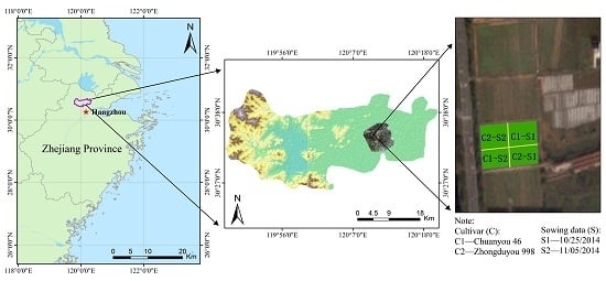
The field campaigns were conducted in Deqing County (Figure 1), an agricultural area located in Zhejiang Province, southeast China. This area is characterized by a subtropical humid monsoon climate with mean annual temperatures between 13 °C and 16 °C and annual precipitation of 1379 mm. Paddy rice is the main summer crop, whereas oilseed rape is the main crop in winter. The experimental field is centered at latitude 30°33′55.5″N, and longitude 120°10′48.42″E. The area has an average elevation of about 20 m above sea level. The experiment was carried out during the 2014–2015 growing season with two cultivars (Chuanyou 46 and Zhongduyou 998) at two sowing dates (25 October 2014 and 5 November 2014). The seeds were sown by broadcasting. Field management practices such as fertilization and herbicide application, and pest and disease control were conducted in line with local agronomic standards. As a dry land crop, no irrigation was applied on oilseed rape plots throughout the growing season.

2.2. Ground LAI Measurements

Plant (oilseed rape) samples were collected to determine LAI using a quadrat scale of 0.5 m× 0.5 m. Due to the relatively high sowing density and canopy volume of oilseed rape in the later stages of growth, only one-quarter of the area of the quadrat scale was used to collect plant samples. Five samples were taken from each plot using the above dimensions. This resulted in a total of 72 samples being sampled (from the original 80 samples, 8 samples showed poor quality and had to be discarded). The geographic locations of these sample points were collected using a Differential Global Positioning System device. The collected samples were transported indoors, and green leaves were separated and scanned using the LI-3000 leaf area meter (Li-Cor, Lincoln, NE, USA). LAI values were calculated by dividing the total leaf area by the corresponding ground sampling area. The LAI measurements of each campaign are listed in

Table 1. Summary of LAI Measurements.

Growth Stage	Acquisition Date	LAI Measurements
		Number of Samples	Mean Value	Value Range	Standard Deviation
Seedling	8 December 2014	18	0.254	0.039–0.713	0.171
Seedling	31 December 2014	20	0.379	0.056–1.096	0.342
Seedling	5 February 2015	16	1.077	0.215–1.844	0.514
Budding	12 March 2015	18	2.302	0.584–3.913	0.931

.

2.3. Satellite Image Acquisition and Processing

Four high spatial resolution satellite images corresponding to dates of field observations have been acquired during the growing season. Due to the generally unfavorable weather conditions (persistent clouds) for optical sensors in the test site, it is extremely difficult to acquire image data from a single optical sensor at periods consistent or coincidental with ground measurements. Hence, we have employed in this study, a multi-source satellite data acquisition approach, so as to overcome the problem of missing temporal data associated with the use of a single sensor, at important crop phonological stages. WV-2, launched in October 2009, is the first high-resolution eight-band multispectral commercial satellite. WV-3, launched in 2014, brings the spatial and spectral resolution to extraordinary levels with eight visible to near-infrared bands (0.42 to 1.04  μm) and eight shortwave infrared bands (1.2 to 2.33 μm). More information on WV-2 and WV-3 can be found on the web pages of Digital Globe Inc. (Oakland, CA, USA) (http://www.digitalglobe.com/). The Pleiades-1A satellite sensor was successfully launched on 16 December 2011 and provides 0.5 m panchromatic and 2 m multispectral image data. This satellite is capable of providing daily revisit cycles for any point on Earth and it covers a total of one million square kilometers (approximately 386,102 square miles). SPOT-6 was successfully launched on 9 September 2012 and is capable of imaging the Earth with a resolution of 1.5 m panchromatic and 6 m multispectral data. Detailed literature on Pleiades-1A and SPOT-6 can be found at (http://www.intelligence-airbusds.com/cn/). In this study, the four visible near-infrared (VNIR) spectral bands (blue, green, red, and near-infrared) of all the sensors above were used to calculate the VIs. A summary of the acquired satellite data is given in

Table 2. Summary of Acquired Satellite Data.

Sensor	Acquisition Date	Spectral Range (μm)				Spatial Resolution (m)	Swath Width (km)
		Blue	Green	Red	Near-Infrared
Pleiades-1A	4 December 2014	0.430–0.550	0.490–0.610	0.600–0.720	0.750–0.950	2	20.0
WV-3	31 December 2014	0.450–0.510	0.510–0.580	0.630–0.690	0.770–0.895	2	13.1
SPOT-6	12 February 2015	0.455–0.525	0.530–0.590	0.625–0.695	0.760–0.890	6	60.0
WV-2	10 March 2015	0.450–0.510	0.510–0.580	0.630–0.690	0.770–0.895	2	16.4

.

To conduct a quantitative analysis of the remote sensing data, the images used in this study were converted from digital numbers to surface reflectance using the ENVI 5.1 software. Like most optical remote sensing data, conventional preprocessing procedures are applicable to these high spatial resolution images. The preprocessing procedures employed in this study include: (1) radiometric calibration of each band, with the necessary coefficients for radiometric calibration derived from the corresponding metadata file; (2) atmospheric correction was performed using the FLAASH (fast line-of-sight atmospheric analysis of spectral hypercubes) module, which is embedded in the ENVI software; and (3) even though geometric correction was not implemented due to the relatively low and flat topography of the test site, using WV-3 as master image, co-registration was performed to ensure the temporal consistency of pixel locations. For Pleiades-1A, WV-3 and WV-2, a 3 × 3 pixel window was used to extract the spectra while one pixel window was used to extract the spectra for SPOT-6. The average reflectance from nine pixels was regarded as corresponding to a ground sample point.

2.4. PROSAIL Model and Simulated Dataset

We have employed in this study, the widely used PROSAIL radiative transfer model [12], which is a combination of the PROSPECT leaf optical property model [26] and the SAIL canopy reflectance model [25]. This coupled modelling scheme has already been applied with success to a number of crops such as wheat, maize, rice, and soybean [28,29,30,31]. In our study, PROSAIL5B was used to simulate the canopy reflectance spectra of oilseed rape [32,33]. The main parameters of the model are shown in

Table 3. Range and Distribution of Radiative Transfer Model Input Variables.

Model	Variable	No. Class	Min	Max	Mean	Std.Dev.
PROSPECT-5B	Leaf chlorophyll content (μg/cm2)	3	25	75	40	20
	Leaf carotenoid content (μg/cm2)	2	5	20	10	7
	Brown pigment content (arbitrary units)	1	0	1.5	0	0.2
	Equivalent water thickness (cm)	2	0	0.05	0.02	0.025
	Dry matter content (g/cm2)	2	0.003	0.02	0.007	0.003
	Leaf structure parameter (unitless)	3	1	2.5	1.5	1
4SAIL	Leaf area index (unitless)	6	0	4	1.3	1
	Average leaf angle (°)	3	30	80	50	10
	Hot spot parameters (m/m)	1	0.1	0.5	0.3	0.2
	Soil brightness (unitless)	2	0	1	0.5	0.5

. The wavelength range of the simulated canopy spectra generated by PROSAIL5B is from 400 to 2500 nm at 1 nm steps.

Truncated Gaussian distribution was used to generate the necessary parameters. Table 3 shows the range and distribution of each PROSAIL input parameter. The individual settings are based on experiences and empirical values from several studies [16,17]. Because it has only a very small influence on canopy reflectance, the skyl parameter (unitless) was constantly set to 10% across all wavelengths. A full orthogonal experimental plan was adopted to combine the 10 input variables by splitting the whole range of variation of each variable into a small number of classes (Table 3). For each combination of the input variables, top of canopy reflectance was then computed for each wavelength, and then resampled according to the spectral response function of corresponding image bands. Because the illumination geometry varies from date to date, four simulated datasets were created, each corresponding to a specific date of observation and the associated sun zenith angle. The corresponding solar zenith angle (°) and observer zenith angle (°) are shown in

Table 4. Sun and Observation Angles for Each Image Used in This Study.

Sensor	Sun Zenith (°)	Sun Azimuth (°)	View Zenith (°)	View Azimuth (°)
Pleiades-1A	55.0	161.2	20.9	180.0
WV-3	57.0	157.4	7.5	156.1
SPOT-6	51.6	146.6	26.2	231.7
WV-2	37.8	153.6	18.9	280.5

, and are identical in each of the 2592 combinations. Each simulated dataset was randomly divided into two groups: 1944 simulations were used to construct the regression models and the rest were used as the independent validation subset.

2.5. Vegetation Indices and Inversion Algorithms

Nine commonly used VIs were calculated in this study (

Table 5. Summary of the Nine Vegetation Indices Tested in this Analysis.

Vegetation Index	Full Name	Formula	Reference
SR	Simple ratio vegetation index	$\frac{{\rho }_{NIR}}{{\rho }_R}$	Jordan [43]
NDVI	Normalized difference vegetation index	$\frac{\left({\rho }_{NIR}-{\rho }_R\right)}{\left({\rho }_{NIR}+{\rho }_R\right)}$	Rouse et al. [44]
PVI	Perpendicular vegetation index	$\frac{\left({\mathsf{\rho }}_{\mathrm{NIR}}-{\mathrm{a}*\mathsf{\rho }}_{\mathrm{R}}-\mathrm{b}\right)}{\sqrt{{\mathrm{a}}^2+1}}$	Huete et al. [45]
SAVI	Soil-adjusted vegetation index	$\frac{\left(1+L1\right)\left({\rho }_{NIR}-{\rho }_R\right)}{\left({\rho }_{NIR}+{\rho }_R+L1\right)}$	Huete [46]
NLI	Nonlinear vegetation index	$\frac{\left({\rho }_{NIR}^2-{\rho }_R\right)}{\left({\rho }_{NIR}^2+{\rho }_R\right)}$	Gong et al. [47]
MSR	Modified simple ratio vegetation index	$\frac{\left(\frac{{\rho }_{NIR}}{{\rho }_R}-1\right)}{\left(\sqrt{\frac{{\rho }_{NIR}}{{\rho }_R}}+1\right)}$	Chen [48]
TSAVI	Transformed soil-adjusted vegetation index	$\frac{a*\left({\rho }_{NIR}-a*{\rho }_R-b\right)}{\left[a*{\rho }_{NIR}+{\rho }_R-a*b+X*\left(1+a^2\right)\right]}$	Baret and Guyot [49]
EVI	Enhanced vegetation index	$\frac{G*\left({\rho }_{NIR}-{\rho }_R\right)}{\left({\rho }_{NIR}+C1*{\rho }_R-C2*{\rho }_B+L2\right)}$	Liu and Huete [50]
ARVI	Atmospherically resistant vegetation index	$\frac{\left({\rho }_{NIR}-{\rho }_R+\gamma *\left({\rho }_B-{\rho }_R\right)\right)}{\left({\rho }_{NIR}+{\rho }_R-\gamma *\left({\rho }_B-{\rho }_R\right)\right)}$	Kaufman and Tanré [51]

Note: ${\rho }_{NIR}, {\rho }_R, {\rho }_B$ represent reflectance in near-infrared, red, blue bands, respectively. a is the slope of the soil line (0.7601), and b is the soil line intercept (0.2343), L1 = 0.5, L2 = 1, G = 2.5, C1 = 6, C2 = 7.5, X = 0.08, $\mathsf{\gamma }=1$.

). These indices have been effectively and successfully used to estimate and map vegetation canopy LAI from moderate and high resolution multispectral remote sensing data [3,34,35]. To identify the optimal VIs for LAI estimation using the simulated datasets, five curve-fitting models were established for each VI at each growth stage. The curve fitting models include linear regression, logarithmic regression, quadratic regression, power regression, and exponential regression. The optimal model was determined based on predicted root mean squared error (RMSE) and the relative root mean square error (RRMSE) (i.e., RMSE divided by the sample mean and multiplied by 100). The process was performed using the cftool toolbox in the MATLAB environment.

In addition to parametric regression, two types of machine learning methods namely, kNN and RFR were used to construct the relationship between VIs and LAI values from simulated datasets. kNN as a non-parametric technique has been used in statistical estimation since the early 1970s [36]. The basic theory behind kNN is that it finds a group of k samples that are closest to the unknown sample in the calibration set based on a similarity measure (e.g., distance functions) and calculates the average of the response variables of the k-nearest neighbor as the predicted value of unknown samples. The parameter k was determined using a repeated cross-validation procedure.

Random forest is an ensemble learning technique developed by Breiman [37] to improve the classification and regression trees (CART) method by combining a large set of decision trees. Three parameters need to be optimized in random forest: ntree, the number of regression trees grown based on a bootstrap sample with replacement of the observations; mtry, the number of different independents tested at each node; and node size, the minimal size of the terminal nodes of the trees. To find ntree and mtry values that can best predict oilseed rape LAI, the two parameters (mtry and ntree) were optimized based on the root mean square error of calibration (RMSEC). The ntree values were tested from 500 to 9500 with 1000 intervals [38], while mtry was tested from 1 to 9 using a single interval. The default nodesize was accepted throughout the analysis [39]. The importance of each predictor was measured by calculating the percentage increase in mean squared error (%IncMSE) when OOB data (out of bag: the samples not in the bootstrap sample) for each variable are permuted, while all others are unchanged. These variable importance values were then used to rank the predictors in terms of the strength of their relationship to response variables.

After ranking the predictor variables with random forest, the challenge was to select the fewest number of predictors that offer the best predictive power and help in the interpretation of the final model [40]. In this regard, a backward feature elimination method (BFE) integrated with RFR as part of the evaluation process was implemented [41,42]. The method starts with all VIs and then progressively eliminates the least promising predictive variables (VIs). At each iteration (n = 9), the model is optimized by selecting the best mtry and ntree, the least promising predictive variable is eliminated and the five cross-validated root mean square error of calibration (RMSECV) is calculated. The smallest subset of variables with the lowest RMSECV was then selected to predict oilseed rape LAI. The kNN and RFR were performed using caret and randomForest packages developed in R software (version 3.3.0; Team 2014), respectively.

3. Results

3.1. LAI Estimation Using Single Independent Variables

Using the simulated datasets, the performance of independent variables for LAI estimation for each growth stage was obtained and the regression results of only the optimal three VIs of each growth stage are shown in

Table 6. Curve Fitting Results of Optimal Three VIs of Each Growth Stage for Oilseed Rape LAI Estimation

Acquisition Date	Predictor Variable	Model	Fitting Equation	R2	RMSE	RRMSE (%)
4 December 2014	MSR	Linear	1.731x + 0.186	0.783	0.474	47.4
		Logarithmic	1.280Log(x) + 2.165	0.878	0.355	35.5
		Quadratic	−1.341x2 + 4.285x − 0.695	0.884	0.346	34.6
		Power	2.001x0.771	0.817	0.445	44.5
		Exponential	0.829exp(0.780x)	0.668	0.596	59.6
	NDVI	Linear	4.706x − 0.679	0.875	0.359	35.9
		Logarithmic	1.848Log(x) + 3.192	0.872	0.364	36.4
		Quadratic	−2.130x2 + 6.691x − 1.046	0.883	0.348	34.8
		Power	4.280x1.388	0.859	0.387	38.7
		Exponential	0.407exp(2.638x)	0.797	0.468	46.8
	ARVI	Linear	4.084x − 0.080	0.861	0.379	37.9
		Logarithmic	1.126Log(x) + 2.959	0.853	0.390	39.0
		Quadratic	−2.599x2 + 6.182x − 0.357	0.879	0.354	35.4
		Power	3.867x0.958	0.864	0.379	37.9
		Exponential	0.604exp(2.187x)	0.773	0.494	49.4
31 December 2014	NDVI	Linear	4.310x − 0.427	0.842	0.404	40.4
		Logarithmic	1.697Log(x) + 3.140	0.865	0.374	37.4
		Quadratic	−3.769x2 + 7.868x − 1.086	0.870	0.367	36.7
		Power	3.887x1.162	0.831	0.425	42.5
		Exponential	0.524exp(2.238x)	0.749	0.519	51.9
	ARVI	Linear	3.744x + 0.204	0.819	0.432	43.2
		Logarithmic	0.848Log(x) + 2.851	0.834	0.414	41.4
		Quadratic	−3.831x2 + 6.743x − 0.154	0.864	0.375	37.5
		Power	3.568x0.730	0.847	0.401	40.1
		Exponential	0.759exp(1.869x)	0.720	0.548	54.8
	MSR	Linear	1.461x + 0.445	0.709	0.549	54.9
		Logarithmic	1.162Log(x) + 2.178	0.857	0.384	38.4
		Quadratic	−1.329x2 + 4.183x − 0.530	0.858	0.384	38.4
		Power	2.027x0.646	0.777	0.490	49.0
		Exponential	0.966exp(0.631x)	0.600	0.651	65.1
12 February 2015	NDVI	Linear	4.355x − 0.459	0.866	0.372	37.2
		Logarithmic	1.663Log(x) + 3.117	0.874	0.361	36.1
		Quadratic	−2.936x2 + 7.090x − 0.950	0.883	0.348	34.8
		Power	3.955x1.206	0.854	0.395	39.5
		Exponential	0.495exp(2.325x)	0.778	0.490	49.0
	MSR	Linear	1.514x + 0.387	0.742	0.517	51.7
		Logarithmic	1.157Log(x) + 2.176	0.875	0.360	36.0
		Quadratic	−1.285x2 + 4.105x − 0.525	0.879	0.354	35.4
		Power	2.019x0.668	0.804	0.461	46.1
		Exponential	0.938exp(0.657x)	0.627	0.630	63.0
	ARVI	Linear	3.829x + 0.157	0.847	0.398	39.8
		Logarithmic	0.814Log(x) + 2.822	0.836	0.413	41.3
		Quadratic	−3.250x2 + 6.331x − 0.129	0.879	0.354	35.4
		Power	3.635x0.765	0.867	0.374	37.4
		Exponential	0.722exp(1.956x)	0.750	0.519	51.9
10 March 2015	NDVI	Linear	4.769x − 0.393	0.815	0.438	43.8
		Logarithmic	1.789Log(x) + 3.399	0.860	0.381	38.1
		Quadratic	−6.476x2 + 10.419x − 1.391	0.864	0.376	37.6
		Power	4.310x1.109	0.805	0.458	45.8
		Exponential	0.579exp(2.329x)	0.711	0.557	55.7
	ARVI	Linear	4.216x + 0.310	0.784	0.472	47.2
		Logarithmic	0.857Log(x) + 3.019	0.835	0.414	41.4
		Quadratic	−6.478x2 + 8.651x − 0.170	0.856	0.386	38.6
		Power	3.876x0.667	0.830	0.425	42.5
		Exponential	0.844exp(1.989x)	0.678	0.586	58.6
	MSR	Linear	1.928x + 0.386	0.697	0.560	56.0
		Logarithmic	1.283Log(x) + 2.463	0.845	0.401	40.1
		Quadratic	−2.309x2 + 5.689x − 0.737	0.851	0.393	39.3
		Power	2.365x0.684	0.756	0.513	51.3
		Exponential	0.955exp(0.819x)	0.585	0.663	66.3

. To identify the high performance variables for LAI estimation, we ranked all variables according to predicted RMSE and RRMSE values in ascending order. NDVI, MSR, and ARVI appeared at the top of the ranking for every growth stage, indicating that these three predictor variables have a good relationship with LAI. The accuracies of TSAVI and PVI for LAI estimation were poor. Thus, to retrieve LAI from predictor variables, variable screening is necessary to ensure a higher accuracy. In addition, the quadratic equations were the optimal models for the best three VIs, which indicates that the non-linear relationships between LAI and VIs were most suitable for different growth stages.

3.2. LAI Estimation Using Simulated Spectral Data and Machine Learning Methods

3.2.1. Optimization of Key Parameters of Random Forest

The results of random forest parameters (mtry and ntree) are shown in Figure 2. The optimization was done using the calibration datasets (n = 1944) and RMSEC. Figure 2 clearly indicates that random forest parameters (ntree and mtry) affect the error of prediction. The optimal combination of ntree and mtry for the four growth stages in our case were 1500/2, 7500/6, 6500/1, and 8500/2, respectively.

3.2.2. Variable Importance Measures

The OOB estimates of error rate were used to measure the importance of VIs. The random forest model was able to explore and rank the predictors by their importance in estimating LAI. Figure 3 shows the variable importance measured in terms of the increase of OOB error, which represents the deterioration of the predictive performance of the model when each predictor is permuted. Among the predictors (VIs), TSAVI made the most notable contribution to the estimation accuracy of oilseed rape LAI at all growth stages.

The variable selection method used in this study was able to identify the smallest number of VIs that would offer the best predictive ability of the random forest. It is worth noting that RMSECV generally decreased as the least important variables were discarded progressively. The use of five, three, five, and one variable (VIs) respectively, for Pleiades-1A, WV-3, SPOT-6, and WV-2 simulated datasets, produced the lowest RMSECV using five-fold cross validation, while the use of all variables (n = 9) produced the highest RMSECV for all simulation datasets (Figure 4).The optimal variables were SR, PVI, MSR, TSAVI, and ARVI for the Pleiades-1A dataset; SR, NDVI, and TSAVI for the WV-3 dataset; SR, NDVI, NLI, MSR, and TSAVI for the SPOT-6 dataset; and MSR for the WV-2 dataset. These selected VIs were then used as input predictive variables in kNN and RFR to predict oilseed rape LAI using the validation datasets.

3.2.3. Predictive Performance of the Machine Learning Methods

The best variables selected by RFR and BFE methods were assessed using the independent validation datasets and the results are displayed in

Table 7. Machine learning results of simulated spectral data for oilseed rape LAI estimation using the optimal variables selected by RFR and validation datasets.

Acquisition Date	Algorithm	Independent Validation Dataset
		Number of the Best Variables	R2	RMSE	RRMSE (%)
4 December 2014	kNN	5	0.984	0.127	6.7
	RFR	5	0.994	0.078	4.2
31 December 2014	kNN	3	0.994	0.082	4.4
	RFR	3	0.997	0.060	3.2
12 February 2015	kNN	5	0.992	0.090	4.8
	RFR	5	0.998	0.051	2.7
10 March 2015	kNN	1	0.924	0.281	14.9
	RFR	1	0.954	0.218	11.6

. Compared to curve fitting, the accuracies of kNN and RFR using the independent validation set were generally better, as indicated by a higher R², and lower RMSE and RRMSE values. This result suggests that the RFR and kNN algorithms are better methods for modeling oilseed rape LAI values from VIs compared to the curving fitting method. In addition, the RFR algorithm consistently produced higher predicted accuracy than kNN for all simulated datasets, which suggests that RFR is the best modeling method in current study.

3.3. Validation of Inversion Models with High Spatial Resolution Images

3.3.1. LAI Map Using Pleiades-1A, WV-2, SPOT-6, and WV-3

The mapping results based on the RFR model established by the best variables are shown in Figure 5. To facilitate visual interpretation of the remote sensing images, the mapping results were divided into five levels of color density indicating the spatio-temporal variability of oilseed rape LAI. Images with a spatial resolution of 2 m presented more elaborate intra-field variations of LAI than images with a spatial resolution of 6 m (Figure 5). This implies that spatial resolution has an important effect on the estimation of LAI. With the growth of oilseed rape, the plots with relatively earlier sowing dates had higher LAI values than plots with later sowing dates. There is an obvious overestimation of LAI for the image on 4 December 2014.

3.3.2. Validation of LAI Using Ground Data

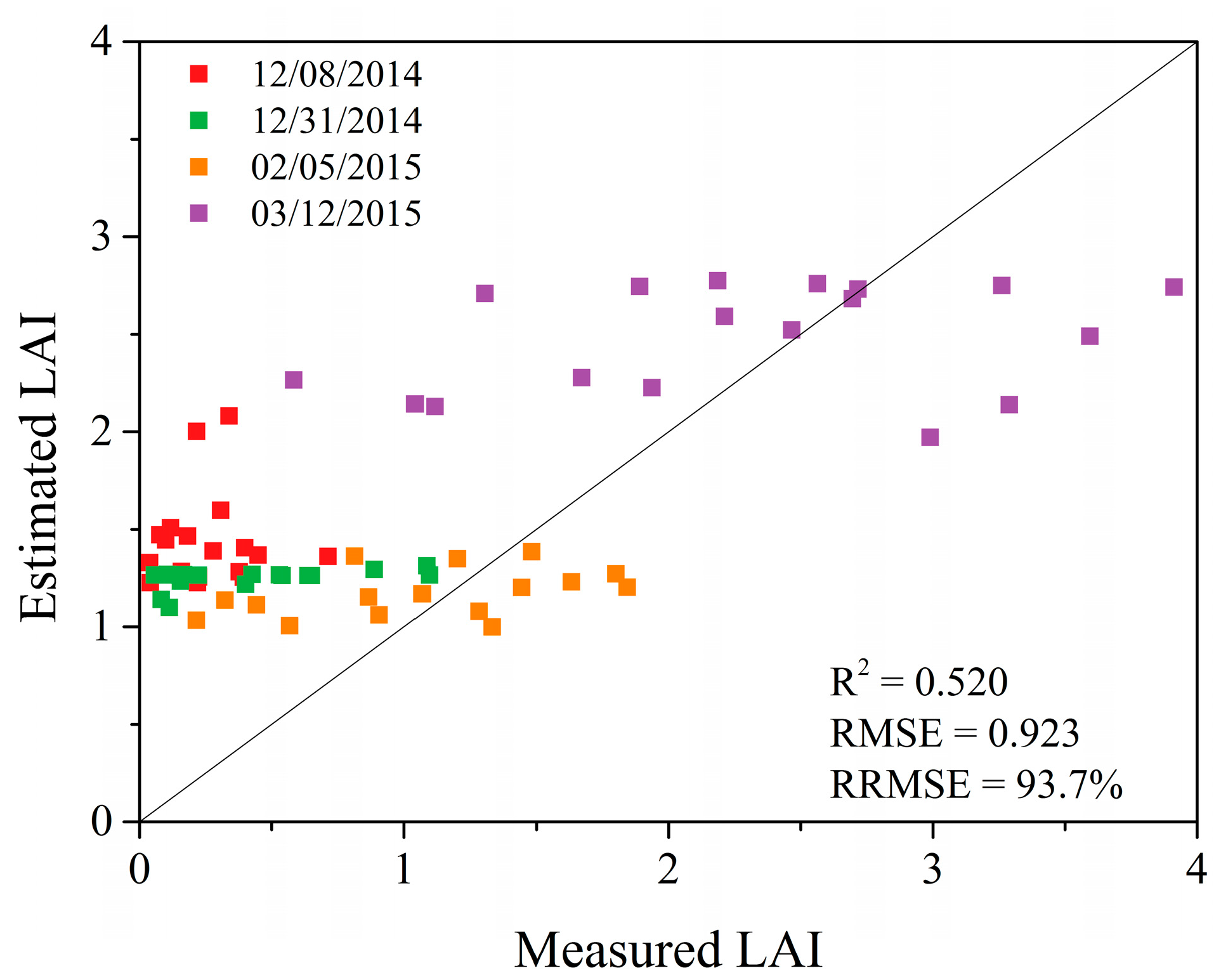
All ground-measured LAI samples acquired synchronously with remote sensing images were used for validation. The relationships between the measured and estimated LAI values are illustrated in Figure 6. The prediction accuracy for estimating LAI was relatively poor with an overall accuracy of R² = 0.520 and RMSE = 0.923 (RRMSE = 93.7%) based on 72 samples. There is an overestimation of LAI in first two observation dates, particularly for the observation on 8 December 2014.

4. Discussion

In this study, LAI values of oilseed rape were estimated using a hybrid inversion method based on a radiative transfer model. This method differs from empirical approaches that require several ground measured datasets for modeling. The hybrid inversion method employed in this study utilizes only a few ground measured biophysical data points to validate the accuracy of the model established with the simulation dataset. In contrast to other inversion strategies based on radiative transfer models, such as look up table, the hybrid inversion method has a greater potential for estimating crop biophysical parameters as the model construction is fast and simple, and the computation time is short with no need to consider the selection of optimal solutions.

The ranking of the three VIs (NDVI, MSR, and ARVI) selected by the curve fitting method at different growth stages was not consistent. The possible reason for this inconsistency is that the performance of VIs can be affected by sun and sensor geometry [52]. Many studies have assessed the effects of viewing and illumination geometry on VIs [53,54,55]. The impacts further hamper the interpretation of temporal variations in land-surface vegetation. In addition, the difference among the spectral response function of the four sensors used in this paper was another reason for this inconsistency. The quadratic equations were the optimal models for the best three VIs. Similar results were reported by Chen, et al. [56] who found the non-linear relationship between LAI and SR to be appropriate for agricultural crops in Landsat-5 Thematic Mapper (TM) scenes.

While VIs derived from satellite remote sensing have been used to map LAI, a drawback is that the general applicability of these regression approaches is reduced because the VIs are affected by many factors including atmospheric effects, canopy geometry, vegetation developmental stage, geometry of observation, understory vegetation and soil conditions, and type of sensors [9,49,57]. An ideal VI should be sensitive to the biophysical parameters of interest but insensitive to confounding factors. Thus, the sensitivity analysis of VIs is very important to obtain an accurate LAI estimate. In this paper, the optimal VIs were selected using curve fitting and random forest methods, and these VIs showed good accuracy for the estimation of LAI. Although the sensitivity analysis of VIs for oilseed rape LAI estimation was not performed, the methodology used in this paper reasonably estimated oilseed rape LAI and is therefore recommended for application at larger mapping scales.

To increase the inversion accuracy of biophysical parameters, several non-parametric regression methods, such as the kNN algorithm, have been used to build the relationship between the simulated spectral variables (VIs) and the crop biophysical parameters of interest [17,21]. These algorithms differ from ordinary least square regressions which need assumptions on the distribution of response variables. In this paper, RFR is regarded as the optimal method to establish the relationship between simulated VIs and LAI values, with a higher R², and lower RMSE and RRMSE values based on the simulated independent validation dataset (Table 7). This finding is consistent with recent studies which indicated the RFR algorithm to be a better alternative to other regression algorithms [52,53]. Random forest is not only used to predict biophysical variables of crops, but also provides an effective methodology for variable selection. The variable importance measure provided by random forest can be used to identify variables that are of relevance and explain the relationship between predictor and response variables. However, after the initial selection of optimal predictor variables, it would still be unclear as to which variable combination is best for the prediction of parameters such as oilseed rape LAI. To find the best subsets of variables, the backward elimination was used and integrated with the variable importance measure. This method has the advantage of shorter computational time while being robust against the problem of data over-fitting. Despite the overwhelming advantages of RFR models as detailed in [37], they also have limitations, especially with respect to the manner in which regression trees are constructed. In this study, random forest is prone to underestimation at high LAI values. This phenomenon has also been observed in [41] where the random forest algorithm, applied to wetland vegetation, exhibited gross underestimation at higher levels of plant biomass.

Four images with high spatial resolution were used to map the temporal and spatial distribution of oilseed rape LAI values in this study. The images with a spatial resolution of 2 m achieved more elaborate information on LAI distribution than images with a spatial resolution of 6 m (Figure 5). The validation result obtained using the optimal modeling algorithms and the optimal VIs displayed a relatively poor prediction accuracy. The image on 4 December 2014 showed an overestimation of LAI values and the validation results from the ground measured dataset also indicated that LAI values from observations on 8 December 2014 and 31 December 2014 were overestimated. The reason for this phenomenon is attributable to the growth of grass in the field which contributes to the pixel values of images. Although herbicides have been applied at the start of the seedling stage, there were still several grasses in the field as observed during in situ measurements. As a result, the retrieved LAI included oilseed rape and grass. Although the overall validation accuracy seems relatively poor in the current study, observations obtained on 5 February 2015 and 12 March 2015 were more close to the one to one line, which indicates the potential of high spatial resolution satellite data for monitoring intra-field variations of crop biophysical parameters, especially from the middle to the latter growth stages. This result is in line with previous studies which have demonstrated that high spatial resolution optical satellite imagery are an efficient data source for the estimation of crop biophysical and biochemical parameters [58,59,60] and their accurate quantification would help to improve the management of crops and agricultural lands.

5. Conclusions

The current study proposed a hybrid inversion method that combines the PROSAIL model and curve fitting and machine learning methods for oilseed rape LAI estimation. The inversion method was verified using field-observed data and high spatial resolution satellite data acquired at a lowland agro-ecology located in southeast China. Nine VIs were calculated and selected using curve fitting and random forest methods based on the PROSAIL model simulation datasets. The result showed that RFR is the optimal method for regression modeling of LAI with an accuracy of R² > 0.954 and RMSE < 0.218. The inversion performance was verified using ground measured LAI data and the corresponding satellite images. The resultant LAI maps confirmed the feasibility of estimating oilseed rape LAI (R² = 0.520, RMSE = 0.923, RRMSE = 93.7%) with high spatial resolution satellite data using VIs and a hybrid inversion method. With our use of multi-source and high spatial resolution satellite data, this contribution would provide a basis for more accurate oilseed rape LAI retrievals at field or parcel scales. Such information could be useful for crop management practices and yield estimation.

References

1. Gholz, H.L.; Vogel, S.A.; Cropper, W.P.; McKelvey, K.; Ewel, K.C.; Teskey, R.O.; Curran, P.J. Dynamics of canopy structure and light interception in Pinus-elliottii stands, North Florida. Econ. Monogr. 1991, 61, 33–51. [Google Scholar] [CrossRef]
2. Chen, J.M.; Black, T.A. Defining leaf-area index for non-flat leaves. Plant Cell Environ. 1992, 15, 421–429. [Google Scholar] [CrossRef]
3. Pu, R.L.; Cheng, J. Mapping forest leaf area index using reflectance and textural information derived from WorldView-2 imagery in a mixed natural forest area in Florida, US. Int. J. Appl. Earth Obs. Geoinf. 2015, 42, 11–23. [Google Scholar] [CrossRef]
4. Alton, P.B. The sensitivity of models of gross primary productivity to meteorological and leaf area forcing: A comparison between a penman-monteith ecophysiological approach and the MODIS light-use efficiency algorithm. Agric. For. Meteorol. 2016, 218, 11–24. [Google Scholar] [CrossRef]
5. Anderson, M.C.; Zolin, C.A.; Sentelhas, P.C.; Hain, C.R.; Semmens, K.; Yilmaz, M.T.; Gao, F.; Otkin, J.A.; Tetrault, R. The evaporative stress index as an indicator of agricultural drought in Brazil: An assessment based on crop yield impacts. Remote Sens. Environ. 2016, 174, 82–99. [Google Scholar] [CrossRef]
6. Weiss, M.; Baret, F.; Smith, G.J.; Jonckheere, I.; Coppin, P. Review of methods for in situ leaf area index (LAI) determination PartII. Estimation of LAI, errors and sampling. Agric. For. Meteorol. 2004, 121, 37–53. [Google Scholar] [CrossRef]
7. Jonckheere, I.; Fleck, S.; Nackaerts, K.; Muys, B.; Coppin, P.; Weiss, M.; Baret, F. Review of methods for in situ leaf area index determination—Part I. Theories, sensors and hemispherical photography. Agric. For. Meteorol. 2004, 121, 19–35. [Google Scholar] [CrossRef]
8. Gower, S.T.; Kucharik, C.J.; Norman, J.M. Direct and indirect estimation of leaf area index, fAPAR, and net primary production of terrestrial ecosystems. Remote Sens. Environ. 1999, 70, 29–51. [Google Scholar] [CrossRef]
9. Kamal, M.; Phinn, S.; Johansen, K. Assessment of multi-resolution image data for mangrove leaf area index mapping. Remote Sens. Environ. 2016, 176, 242–254. [Google Scholar] [CrossRef]
10. Verrelst, J.; Rivera, J.P.; Veroustraete, F.; Munoz-Mari, J.; Clevers, J.; Camps-Valls, G.; Moreno, J. Experimental Sentinel-2 LAI estimation using parametric, non-parametric and physical retrieval methods—A comparison. ISPRS J. Photogramm. Remote Sens. 2015, 108, 260–272. [Google Scholar] [CrossRef]
11. Yang, F.; Sun, J.L.; Fang, H.L.; Yao, Z.F.; Zhang, J.H.; Zhu, Y.Q.; Song, K.S.; Wang, Z.M.; Hu, M.G. Comparison of different methods for corn LAI estimation over northeastern China. Int. J. Appl. Earth Obs. Geoinf. 2012, 18, 462–471. [Google Scholar]
12. Jacquemoud, S.; Verhoef, W.; Baret, F.; Bacour, C.; Zarco-Tejada, P.J.; Asner, G.P.; Francois, C.; Ustin, S.L. PROSPECT plus SAIL models: A review of use for vegetation characterization. Remote Sens. Environ. 2009, 113, S56–S66. [Google Scholar] [CrossRef]
13. Houborg, R.; Soegaard, H.; Boegh, E. Combining vegetation index and model inversion methods for the extraction of key vegetation biophysical parameters using Terra and Aqua MODIS reflectance data. Remote Sens. Environ. 2007, 106, 39–58. [Google Scholar] [CrossRef]
14. Jacquemoud, S.; Bacour, C.; Poilve, H.; Frangi, J.P. Comparison of four radiative transfer models to simulate plant canopies reflectance: Direct and inverse mode. Remote Sens. Environ. 2000, 74, 471–481. [Google Scholar] [CrossRef]
15. Verrelst, J.; Rivera, J.P.; Leonenko, G.; Alonso, L.; Moreno, J. Optimizing LUT-based RTM inversion for semiautomatic mapping of crop biophysical parameters from Sentinel-2 and-3 data: Role of cost functions. IEEE Trans. Geosci. Remote Sens. 2014, 52, 257–269. [Google Scholar] [CrossRef]
16. Verger, A.; Vigneau, N.; Cheron, C.; Gilliot, J.M.; Comar, A.; Baret, F. Green area index from an unmanned aerial system over wheat and rapeseed crops. Remote Sens. Environ. 2014, 152, 654–664. [Google Scholar] [CrossRef]
17. Verger, A.; Baret, F.; Camacho, F. Optimal modalities for radiative transfer-neural network estimation of canopy biophysical characteristics: Evaluation over an agricultural area with CHRIS/PROBA observations. Remote Sens. Environ. 2011, 115, 415–426. [Google Scholar] [CrossRef]
18. Bacour, C.; Baret, F.; Beal, D.; Weiss, M.; Pavageau, K. Neural network estimation of LAI, fAPAR, fCover and LAIxC(ab), from top of canopy MERIS reflectance data: Principles and validation. Remote Sens. Environ. 2006, 105, 313–325. [Google Scholar] [CrossRef]
19. Atzberger, C. Object-based retrieval of biophysical canopy variables using artificial neural nets and radiative transfer models. Remote Sens. Environ. 2004, 93, 53–67. [Google Scholar] [CrossRef]
20. Kimes, D.S.; Knyazikhin, Y.; Privette, J.L.; Abuelgasim, A.A.; Gao, F. Inversion methods for physically-based models. Remote Sens. Rev. 2000, 18, 381–439. [Google Scholar] [CrossRef]
21. Duveiller, G.; Weiss, M.; Baret, F.; Defourny, P. Retrieving wheat green area index during the growing season from optical time series measurements based on neural network radiative transfer inversion. Remote Sens. Environ. 2011, 115, 887–896. [Google Scholar] [CrossRef]
22. Darvishzadeh, R.; Atzberger, C.; Skidmore, A.; Schlerf, M. Mapping grassland leaf area index with airborne hyperspectral imagery: A comparison study of statistical approaches and inversion of radiative transfer models. ISPRS J. Photogramm. Remote Sens. 2011, 66, 894–906. [Google Scholar] [CrossRef]
23. Vohland, M.; Mader, S.; Dorigo, W. Applying different inversion techniques to retrieve stand variables of summer barley with PROSPECT plus SAIL. Int. J. Appl. Earth Obs. Geoinf. 2010, 12, 71–80. [Google Scholar] [CrossRef]
24. Weiss, M.; Baret, F.; Myneni, R.B.; Pragnere, A.; Knyazikhin, Y. Investigation of a model inversion technique to estimate canopy biophysical variables from spectral and directional reflectance data. Agronomie 2000, 20, 3–22. [Google Scholar] [CrossRef]
25. Verhoef, W. Light-scattering by leaf layers with application to canopy reflectance modeling—The SAIL model. Remote Sens. Environ. 1984, 16, 125–141. [Google Scholar] [CrossRef]
26. Jacquemoud, S.; Baret, F. PROSPECT—A model of leaf optical-properties spectra. Remote Sens. Environ. 1990, 34, 75–91. [Google Scholar] [CrossRef]
27. Moran, M.S.; Inoue, Y.; Barnes, E.M. Opportunities and limitations for image-based remote sensing in precision crop management. Remote Sens. Environ. 1997, 61, 319–346. [Google Scholar] [CrossRef]
28. Nigam, R.; Bhattacharya, B.K.; Vyas, S.; Oza, M.P. Retrieval of wheat leaf area index from AWIFS multispectral data using canopy radiative transfer simulation. Int. J. Appl. Earth Obs. Geoinf. 2014, 32, 173–185. [Google Scholar] [CrossRef]
29. Duan, S.B.; Li, Z.L.; Wu, H.; Tang, B.H.; Ma, L.L.; Zhao, E.Y.; Li, C.R. Inversion of the PROSAIL model to estimate leaf area index of maize, potato, and sunflower fields from unmanned aerial vehicle hyperspectral data. Int. J. Appl. Earth Obs. Geoinf. 2014, 26, 12–20. [Google Scholar] [CrossRef]
30. Darvishzadeh, R.; Matkan, A.A.; Ahangar, A.D. Inversion of a radiative transfer model for estimation of rice canopy chlorophyll content using a Lookup-Table approach. IEEE J. Sel. Top. Appl. Earth Obs. Remote Sens. 2012, 5, 1222–1230. [Google Scholar] [CrossRef]
31. Mridha, N.; Sahoo, R.N.; Sehgal, V.K.; Krishna, G.; Pargal, S.; Pradhan, S.; Gupta, V.K.; Kumar, D.N. Comparative evaluation of inversion approaches of the radiative transfer model for estimation of crop biophysical parameters. Int. Agrophys. 2015, 29, 201–212. [Google Scholar] [CrossRef]
32. Feret, J.B.; Francois, C.; Asner, G.P.; Gitelson, A.A.; Martin, R.E.; Bidel, L.P.R.; Ustin, S.L.; Le Maire, G.; Jacquemoud, S. PROSPECT-4 and 5: Advances in the leaf optical properties model separating photosynthetic pigments. Remote Sens. Environ. 2008, 112, 3030–3043. [Google Scholar] [CrossRef]
33. Verhoef, W.; Jia, L.; Xiao, Q.; Su, Z. Unified optical-thermal four-stream radiative transfer theory for homogeneous vegetation canopies. IEEE Trans. Geosci. Remote Sens. 2007, 45, 1808–1822. [Google Scholar] [CrossRef]
34. Omer, G.; Mutanga, O.; Abdel-Rahman, E.M.; Adam, E. Empirical prediction of leaf area index (LAI) of endangered tree species in intact and fragmented indigenous forests ecosystems using WorldView-2 data and two robust machine learning algorithms. Remote Sens. 2016, 8, 324. [Google Scholar] [CrossRef]
35. Li, X.C.; Zhang, Y.J.; Luo, J.H.; Jin, X.L.; Xu, Y.; Yang, W.Z. Quantification winter wheat LAI with HJ-1CCD image features over multiple growing seasons. Int. J. Appl. Earth Obs. Geoinf. 2016, 44, 104–112. [Google Scholar] [CrossRef]
36. Franco-Lopez, H.; Ek, A.R.; Bauer, M.E. Estimation and mapping of forest stand density, volume, and cover type using the k-nearest neighbors method. Remote Sens. Environ. 2001, 77, 251–274. [Google Scholar] [CrossRef]
37. Breiman, L. Random forests. Mach. Learn. 2001, 45, 5–32. [Google Scholar] [CrossRef]
38. Prasad, A.M.; Iverson, L.R.; Liaw, A. Newer classification and regression tree techniques: Bagging and random forests for ecological prediction. Ecosystems 2006, 9, 181–199. [Google Scholar] [CrossRef]
39. Vincenzi, S.; Zucchetta, M.; Franzoi, P.; Pellizzato, M.; Pranovi, F.; Leo, G.A.D.; Torricelli, P. Application of a Random Forest algorithm to predict spatial distribution of the potential yield of Ruditapes philippinarum in the Venice lagoon, Italy. Ecol. Model. 2015, 222, 1471–1478. [Google Scholar] [CrossRef]
40. Ismail, R.; Mutanga, O.; Woldai, T.; Annegarn, H. A comparison of regression tree ensembles: predicting Sirex noctilio induced water stress in Pinus patula forests of Kwazulu-Natal, South Africa. Int. J. Appl. Earth Obs. Geoinf. 2010, 12, S45–S51. [Google Scholar] [CrossRef]
41. Mutanga, O.; Adam, E.; Cho, M.A. High density biomass estimation for wetland vegetation using WorldView-2 imagery and random forest regression algorithm. Int. J. Appl. Earth Obs. Geoinf. 2012, 18, 399–406. [Google Scholar] [CrossRef]
42. Guyon, I.; Elisseeff, A. An introduction to variable and feature selection. J. Mach. Learn Res. 2003, 3, 1157–1182. [Google Scholar]
43. Jordan, C.F. Derivation of leaf area index from quality of light on forest floor. Ecology 1969, 50, 663–666. [Google Scholar] [CrossRef]
44. Rouse, J.W.; Haas, R.H.; Schell, J.A.; Deering, D.W. Monitoring vegetation systems in the Great Plains with ERTS. In Proceedings of the 3rd ERTS Symposium, Washington, DC, USA, 10–14 December 1973; pp. 309–317. [Google Scholar]
45. Huete, A.R.; Jackson, R.D.; Post, D.F. Spectral response of a plant canopy with different soil backgrounds. Remote Sens. Environ. 1985, 17, 37–53. [Google Scholar] [CrossRef]
46. Huete, A.R. A soil-adjusted vegetation index (SAVI). Remote Sens. Environ. 1988, 25, 295–309. [Google Scholar] [CrossRef]
47. Gong, P.; Pu, R.; Biging, G.S.; Larrieu, M.R. Estimation of forest leaf area index using vegetation indices derived from hyperion hyperspectral data. IEEE Trans. Geosci. Remote Sens. 2003, 41, 1355–1362. [Google Scholar] [CrossRef]
48. Chen, J.M. Evaluation of vegetation indices and a modified simple ratio for boreal applications. Can. J. Remote Sens. 1996, 22, 229–242. [Google Scholar] [CrossRef]
49. Baret, F.; Guyot, G. Potentials and limits of vegetation indices for LAI and APAR assessment. Remote Sens. Environ. 1991, 35, 161–173. [Google Scholar] [CrossRef]
50. Liu, H.Q.; Huete, A. A feedback based modification of the NDVI to minimize canopy background and atmospheric noise. IEEE Trans. Geosci. Remote Sens. 1995, 33, 457–465. [Google Scholar]
51. Kaufman, Y.J.; Tanré, D. Atmospherically resistant vegetation index (ARVI) for EOS-MODIS. IEEE Trans. Geosci. Remote Sens. 1992, 30, 261–270. [Google Scholar] [CrossRef]
52. Xiao, Y.; Zhao, W.; Zhou, D.; Gong, H. Sensitivity analysis of vegetation reflectance to biochemical and biophysical variables at leaf, canopy, and regional scales. IEEE Trans. Geosci. Remote Sens. 2014, 52, 4014–4024. [Google Scholar] [CrossRef]
53. Bhandari, S.; Phinn, S.; Gill, T. Assessing viewing and illumination geometry effects on the MODIS vegetation index (MOD13Q1) time series: Implications for monitoring phenology and disturbances in forest communities in Queensland, Australia. Int. J. Remote Sens. 2011, 32, 7513–7538. [Google Scholar] [CrossRef]
54. Los, S.O.; North, P.R.J.; Grey, W.M.F.; Barnsley, M.J. A method to convert AVHRR normalized difference vegetation index time series to a standard viewing and illumination geometry. Remote Sens. Environ. 2005, 99, 400–411. [Google Scholar] [CrossRef]
55. Middleton, E.M. Solar zenith angle effects on vegetation indexes in tallgrass prairie. Remote Sens. Environ. 1991, 38, 45–62. [Google Scholar] [CrossRef]
56. Chen, J.M.; Pavlic, G.; Brown, L.; Cihlar, J.; Leblanc, S.G.; White, H.P.; Hall, R.J.; Peddle, D.R.; King, D.J.; Trofymow, J.A.; et al. Derivation and validation of Canada-wide coarse-resolution leaf area index maps using high-resolution satellite imagery and ground measurements. Remote Sens. Environ. 2002, 80, 165–184. [Google Scholar] [CrossRef]
57. Vina, A.; Gitelson, A.A. New developments in the remote estimation of the fraction of absorbed photosynthetically active radiation in crops. Geophys. Res. Lett. 2005, 32. [Google Scholar] [CrossRef]
58. Claverie, M.; Demarez, V.; Duchemin, B.; Hagolle, O.; Ducrot, D.; Marais-Sicre, C.; Dejoux, J.F.; Huc, M.; Keravec, P.; Béziat, P. Maize and sunflower biomass estimation in southwest France using high spatial and temporal resolution remote sensing data. Remote Sens. Environ. 2012, 124, 844–857. [Google Scholar] [CrossRef]
59. Hadria, R.; Duchemin, B.; Jarlan, L.; Dedieu, G.; Baup, F.; Khabba, S.; Olioso, A.; Toan, T.L.; Woldai, T.; Annegarn, H.; et al. Potentiality of optical and radar satellite data at high spatio-temporal resolutions for the monitoring of irrigated wheat crops in Morocco. Int. J. Appl. Earth Obs. Geoinf. 2010, 12, S32–S37. [Google Scholar] [CrossRef]
60. Courault, D.; Bsaibes, A.; Kpemlie, E.; Hadria, R.; Hagolle, O.; Marloie, O.; Hanocq, J.; Olioso, A.; Bertrand, N.; Desfonds, V.; et al. Assessing the potentialities of FORMOSAT-2 data for water and crop monitoring at small regional scale in south-eastern France. Sensors 2008, 8, 3460–3481. [Google Scholar] [CrossRef] [PubMed]
Figure 1. Location of the experimental field and distribution of experimental plots. The study area is shown on a Pleiades-1A image acquired on 4 December 2014.
Remotesensing 09 00488 g001
Figure 2. Optimization of random forest parameters (ntree and mtry) using RMSEC. The optimal ntree and mtry that yielded the lowest RMSEC are identified with black arrows.
Remotesensing 09 00488 g002
Figure 3. Measuring the variables (VIs) importance in predicating oilseed rape LAI using RFR method. The models of each growth stage were developed using the optimal combination of mtry and ntree. Higher % IncMSE indicates greater variable importance.
Remotesensing 09 00488 g003
Figure 4. Selecting the optimal number of variables (VIs) using backward elimination search function. The RMSECV is calculated from the calibration datasets (n = 1944) using five-fold cross validation.
Remotesensing 09 00488 g004
Figure 5. Spatial distribution of oilseed rape LAI estimated from high spatial resolution images and optimal VIs (a) SR, PVI, MSR, TSAVI, and ARVI; (b) SR, NDVI, and TSAVI; (c) SR, NDVI, NLI, MSR, and TSAVI; and (d) MSR, respectively, for Pleiades-1A, WV-3, SPOT-6, and WV-2, based on the RFR method.
Remotesensing 09 00488 g005
Figure 6. Relationship between measured oilseed rape LAI values and oilseed rape LAI values estimated using the RFR modelwith the optimal predictive variables.
Remotesensing 09 00488 g006