Article

Retrieving Soybean Leaf Area Index from Unmanned Aerial Vehicle Hyperspectral Remote Sensing: Analysis of RF, ANN, and SVM Regression Models

1
Beijing Research Center for Information Technology in Agriculture, Key Laboratory of Quantitative Remote Sensing in Agriculture, Ministry of Agriculture, Beijing 100097, China
2
School of Surveying and Land Information Engineering, Henan Polytechnic University, Jiaozuo 454000, China
3
National Engineering Research Center for Information Technology in Agriculture, Beijing 100097, China
4
Beijing Engineering Research Center for Agriculture Internet of Things, Beijing 100097, China
*
Author to whom correspondence should be addressed.
Remote Sens. 2017, 9(4), 309; https://doi.org/10.3390/rs9040309
Submission received: 28 December 2016 / Revised: 15 March 2017 / Accepted: 21 March 2017 / Published: 25 March 2017
(This article belongs to the Special Issue Earth Observations for Precision Farming in China (EO4PFiC))

Abstract

:
Leaf area index (LAI) is an important indicator of plant growth and yield that can be monitored by remote sensing. Several models were constructed using datasets derived from SRS and STR sampling methods to determine the optimal model for soybean (multiple strains) LAI inversion for the whole crop growth period and a single growth period. Random forest (RF), artificial neural network (ANN), and support vector machine (SVM) regression models were compared with a partial least-squares regression (PLS) model. The RF model yielded the highest precision, accuracy, and stability with V-R2, SDR2, V-RMSE, and SDRMSE values of 0.741, 0.031, 0.106, and 0.005, respectively, over the whole growth period based on STR sampling. The ANN model had the highest precision, accuracy, and stability (0.452, 0.132, 0.086, and 0.009, respectively) over a single growth phase based on STR sampling. The precision, accuracy, and stability of the RF, ANN, and SVM models were improved by inclusion of STR sampling. The RF model is suitable for estimating LAI when sample plots and variation are relatively large (i.e., the whole growth period or more than one growth period). The ANN model is more appropriate for estimating LAI when sample plots and variation are relatively low (i.e., a single growth period).

Graphical Abstract

1. Introduction

Soybeans are the most widely grown oil crops in the world. Soybean leaf area index (LAI) reflects photosynthetic rate [1,2] and crop yield [3]. Therefore, LAI is an essential parameter for breeding high-yield soybean plants [4,5]. Methods for estimating LAI can be categorized as direct methods and indirect methods [6,7]. Indirect methods adopt devices such as plant canopy analyzers (e.g., LAI-2000, LI-COR, Inc., Lincoln, NE, USA), digital hemispherical photography (DHP), and remote sensing [8]. Remote sensing technology is cost-effective and non-destructive and, thus, a prevalent technology for estimating LAI [9].
Studies have proposed numerous methods for LAI extraction based on observed hyperspectral reflectance bands [10,11], making accurate LAI retrieval a popular theme of remote sensing applications [12]. Retrieval models can be divided into physical models and statistical models [13,14,15,16]. Physical models are often applied to simple homogeneous crops but require several prerequisites (e.g., a homogeneous canopy), specific circumstances, and structural parameters, which limits their application [17,18,19]. Statistical models for LAI retrieval include parametric and non-parametric regression models. Parametric models are simple and easy to understand, but they make poor use of available spectral information and the inversion accuracy is largely dependent on selected bands [16,20]. In contrast, non-parametric regression methods make full use of spectral information and have a high non-linear adaptation; however, one of their main drawbacks is instability when applied to datasets that deviate from the training dataset [21]. Since soybean breeding uses many varieties, we focused on the application of nonparametric models for LAI inversion. Non-parametric regression models have high methodological accuracy and robust performance [16] and, thus, are widely used for physiological and biochemical parameter inversion. For instance, Darvishzadeh et al. used partial least squares regression (PLS) to retrieve chlorophyll content and LAI of heterogeneous grassland canopies, respectively, and the prediction accuracy of LAI was higher than chlorophyll content [22]. Han et al. used random forest (RF) and support vector machine (SVM) methods to invert the canopy LAI of apple trees; the estimation accuracy of the RF model was better than that of the SVM model, and RF was suitable for apple LAI estimation throughout the full fruit growth period [23]. Omer et al. used artificial neural network (ANN) and SVM methods to predict the LAI of six endangered tree species and found that the SVM model had higher prediction accuracy compared with the ANN model [24]. Verrelst et al. used ANN, SVM, nuclear ridge regression (KRR), and Gaussian process regression (GPR) methods to predict LAI and concluded that GPR was a fast and accurate nonlinear retrieval algorithm [25]. Mustafa et al. combined the Bayesian network (BN) method with a forest growth model to improve LAI prediction accuracy [26].
Numerous studies have employed remote sensing to estimate crop LAI, but few have focused on crop-breeding fields (i.e., multiple strains) using different sampling methods [27]. Given that nonparametric models are affected by training sets, previous studies have proposed probabilistic sampling [21], K-fold sampling [28], and Markov Chain Monte Carlo (MCMC) sampling [29] methods. K-fold sampling and MCMC sampling can overcome the influence of data distribution on the calibration set to a certain extent, but the calibration set should be adjusted repeatedly in combination with the model [28], and it is difficult to ensure agreement of the calibration set with the overall data distribution. The least absolute shrinkage and selection operator (LASSO) does not fully utilize hyperspectral data. Bayesian networks cannot ensure that the calibration set distribution is close to the overall data distribution. To overcome these shortcomings, we used two sampling methods (simple random sampling, SRS, and stratified type sampling or stratified sampling, STR) [30] and four nonparametric models (decision tree learning, artificial neural networks, kernel methods, and linear non-parametric models; RF, ANN, SVM, and PLS, respectively) [16] for LAI inversion over a single growth stage and the whole growth stage of multiple strains of soybean plants.
The objective of this study was to comprehensively evaluate the performance of RF, ANN, and SVM models in LAI inversion using hyperspectral data and corresponding ground data for heterogeneous soybean crops. All ground measurements and remote sensing data were collected in Jiaxiang County, Jining City, Shandong Province in 2015. Following a brief introduction on the merits and shortcomings of LAI inversion, the RF, ANN, and SVM regression methods and SRS and STR [30] sampling methods are presented. The theoretical basis and application of the RF, ANN, and SVM methods and the evaluation index are discussed in Section 2. LAI results for the whole growth period from the RF, ANN, and SVM models are presented in Section 3. Finally, the discussion and conclusions of this study are summarized in Section 4 and Section 5, respectively.

2. Materials and Methods

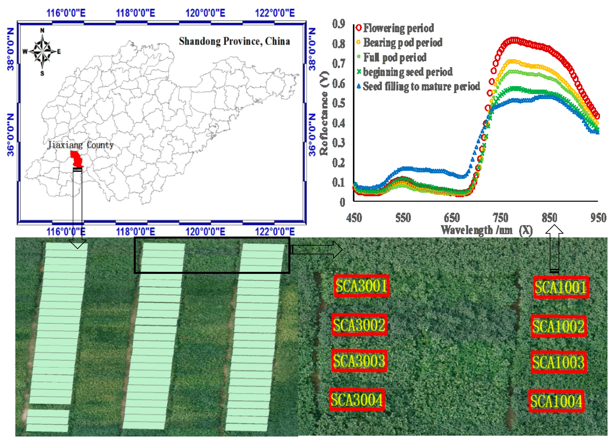
2.1. Study Site and Experimental Design

The experiment was carried out in Jiaxiang County, Jining City, Shandong Province (116°22′10″~116°22′20″E, 35°25′50″~35°26′10″N), located at the junction of the Zhongnan Mountains and the North China Plain (Figure 1). The terrain is mainly composed of plains, is located in the warm temperate zone, and experiences a monsoon continental climate. The average elevation is 35–40 m, the average temperature is 13.3 °C–14.1 °C, the average annual precipitation is 597–820 mm, and the frost-free period is approximately 199 days. A total of 126 sampling plots of hybridized breed combinations were used as the research target. The breed combinations were generated from 46 varieties of soybeans planted on 13 June 2015, using 300 kg/hm2 of compound fertilizer (i.e., 15% NPK) as the base fertilizer and conventional agricultural management practices. Data were collected five times on 1 August 2015 (flowering period, R1), 13 August (bearing period, R3), 1 September (full pod period, R5), 17 September (beginning of the seed period, R6), and 28 September (seed filling to mature stages, R7). Planting density in the test area was approximately 195,000/hm2. There were 126 sampling plots during each growth period.

2.2. Data Collection
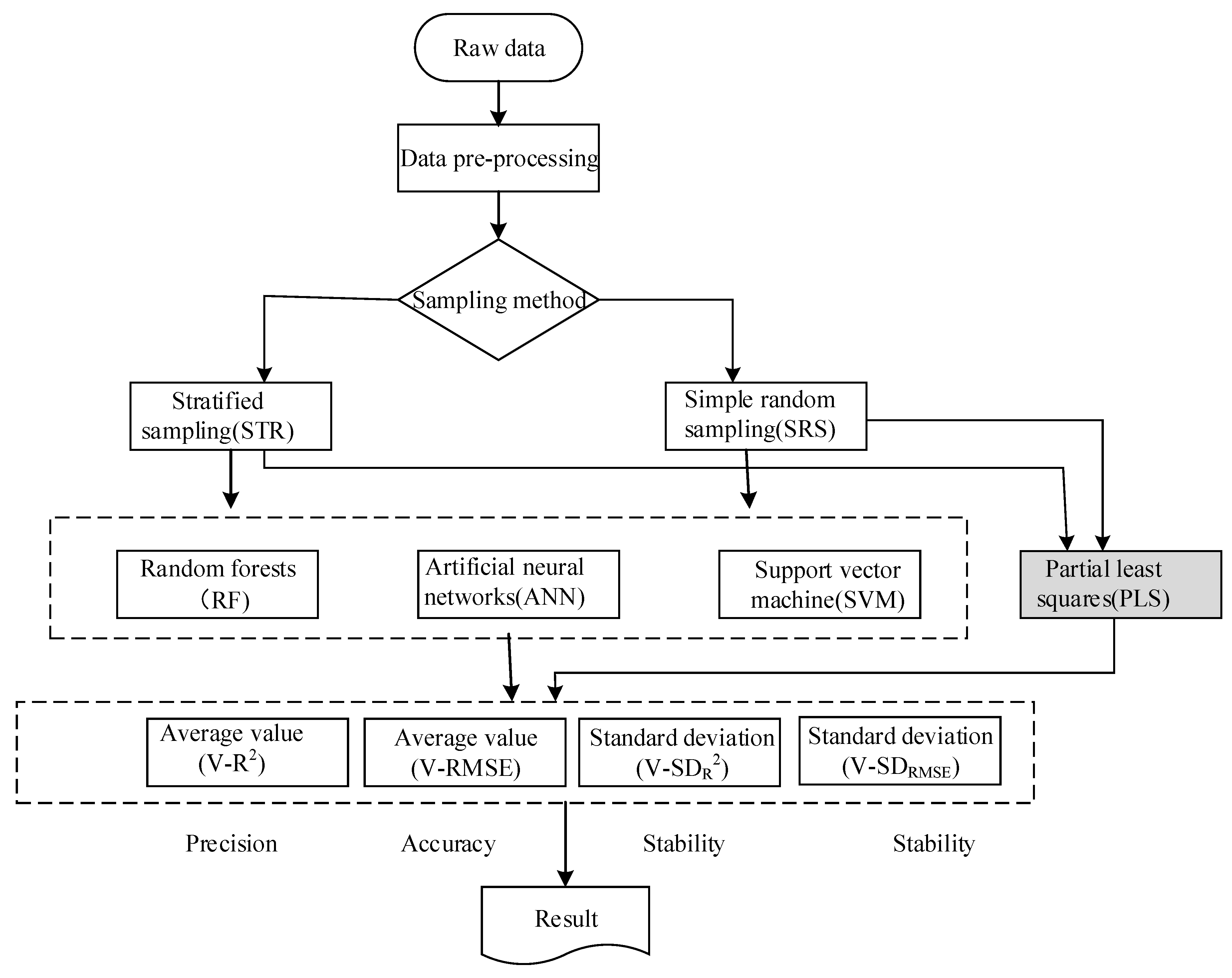
Unmanned aerial vehicles with eight rotors, a maximum load capacity of approximately 6 kg, and a flying altitude ranging from 50 m to 100 m were equipped with a hyperspectral snapshot camera (Cubert GmbH, Ulm, Baden-Württemberg, Germany) and a single Pokini Z small board computer (EXTRA Computer GmbH, Sachsenhausen, Germany). The total weight of the camera was ~470 g, and its housing dimensions were about 28 × 6.5 × 7 cm. The instrument had a spectral range of 450 to 950 nm, a spectral sampling interval of 4 nm, a spectral resolution of 8 nm at 532 nm, and a total of 125 spectral channels. For each band, a 50 × 50 pixel image with a 12 bit (4096 DN) dynamic range was created by projecting different bands to different parts of a charged coupled device (CCD). A grayscale image with a resolution of 990 × 1000 pixels was captured at the same time the HS image was recorded.
Before data collection, a black and white board was used for radiation calibration of the UHD 185. Under the control of Pokini Z software (produced by German Extra Computer Gmbh), data were collected with a sampling interval of 1 m from a height of 50 m and a focal distance of 23 mm. Hyperspectral pixels were acquired with a spatial resolution of 35 cm, and grey-scale pixels were acquired with a spatial resolution of 1.4 cm. Data were stored in the Pokini Z computer, and the ground control station remotely controlled the flight via a wireless network created by Pokini Z [31]. With the camera software, the hyperspectral resolution could be pan-sharpened to the same resolution as the grayscale image. The unmanned aerial vehicles followed the same routes during each of the five growing periods.
Ground data were acquired simultaneously with the unmanned aerial vehicle data. LAI was measured with an LAI-2200C canopy analyzer (produced by the USA Li-Cor, Lincoln, NE, USA) [32]. The instrument uses a “fish-eye” optical sensor with a 270° vertical field of view and a 360° horizontal field of view to measure transmitted light at 5 angles above and below the canopy. The leaf area index was calculated using the radiation transfer model for vegetation canopy. The first order derivatives of 125 spectra were taken to eliminate noise from the soil, resulting in 124 first order derivative spectra [33,34]. A boxplot was used to remove outliers [35,36]. Table 1 shows the distribution of LAI at different growth stages. LAI values were significant (p > 0.05) during the R6 and R3 periods only, indicating that the LAI distribution was unbalanced during most growth periods.
Data distributions influence machine learning [21]. When the population data is uniformly distributed, SRS provides a calibration set that reflects the population data. When the data distribution is unbalanced, it is difficult to produce a good calibration set, but the STR method can avoid this problem [30]. The STR method used in this study divided the overall data into small groups by based on LAI, and a simple random sample was collected from each group. The more stratified the data, the closer a random sample is to the population dataset. However, sampling efficiency and sample representativeness are reduced when the number of strata is less than 30 [37,38]. Every 7–10 days represents one soybean growth period, for a total of approximately 16 periods throughout the whole growth process. Therefore, 543 samples from the whole growth period were divided into 16 layers, with each layer including 34 samples. Sampling points from the full pod grain period (total of 123) were divided into 4 layers with 31 samples per layer. Approximately 70% of the samples collected in 2015 were used for the calibration set, and the remaining samples were used for the validation set [23]. For unbiased evaluation of the RF, ANN, and SVM regression models, the LAI data were normalized before being input into the models.

2.3. Methods

To further study LAI estimation by RF, ANN, and SVM models, the SRS and STR sampling methods were used to produce calibration sets [30]. The calibration set contained 70% of the total samples, and the remaining samples were used as validation set. To explore model performance, LAI inversion was carried out over the whole growth period and a single growth period. The full pod period is the most important period for soybean breeding [27], and LAI during this period is uniformly distributed and similar to distributions during most of the other growth periods. There were some shortcomings in the comparative study of the inverse LAI models for multiple strains used in this study. We only considered the effects of object characteristics (heterogeneous vegetation) and important influential factors (model calibration set) of nonparametric models on LAI model performance. In the next step, we will further compare the performance among Bayesian, Gaussian process regression (GPR), and models combined with sampling methods for physiological and biochemical parameter inversion for multiple soybean strains.
One-hundred and twenty four first order derivative spectra and two sampling methods were used to establish the RF, ANN, and SVM models, and the results reveal the necessary conditions and advantages of the three models. A flowchart is illustrated in Figure 2.

2.3.1. Random Forest Algorithm

The RF algorithm is based on the classification tree algorithm [39]. RF regression uses bootstrap sampling, and each bootstrap sample is used to construct a decision tree. Training samples are constantly selected to minimize the sum of squared residuals until a complete tree is formed. Multiple decision trees are formed, and voting is used to obtain the final prediction [40]. RF models can handle high-dimensional data and evaluate the feature order, which affects the sample classification and limits interactions between features. An advantageous characteristic of RF modeling is that it is not subject to over-fitting [23]. The most important parameter of RF is the number of trees; the more trees, the higher the accuracy of the RF prediction. Sufficient tree size can ensure the diversity of integrated classifiers. The model was established and validated using the RF function in the “randomForest” package [41] within the statistical software package R 3.2.0.

2.3.2. Artificial Neural Network Algorithm

ANN regression is based on the gradient learning method. It is a nonparametric nonlinear model that uses neural network spreading between layers and simulates human brain receivers and information processing [42]. ANN includes an input layer, hidden layer, and output layer, as well as network initialization (i.e., the number of neurons is determined by the input and expected output to initialize weights between neurons), hidden layer, and output layer calculations. The error values and weights are updated to obtain the final weight [43]. ANN is a learning classification method based on large samples and is affected by the complexities of the network structure and the sample, making it prone to over-learning and reducing the ability for generalization. The most important parameter in ANN regression models is the number of neurons; the more neurons, the higher the learning accuracy and the weaker the generalization ability. The model was established and validated by repeatedly using the nnet function in the “nnet” package to determine the suitable number of neurons [44].

2.3.3. Support Vector Machine Algorithm

SVM is a pattern recognition method based on statistical learning theory. SVM was initially used for classification [45] but is now mainly used for classification and regression of small non-linear and high-dimensional samples. SVM is built based on the VC-dimension of statistical learning theory and the minimum structural risk principle. The model learning accuracy is analyzed, and learning is performed without error recognition using limited sample information. The minimum deviation of the hyperplane from the sample points is used to obtain the best universal ability [46]. SVMs include linear and non-linear regressions [47]. Important parameters include the kernel function, which reflects similarity between data points (i.e., between reflectance values) and the cost loss function (regularization parameter) [25]. The radial basis function (RBF) was used as the kernel function, using the ”tune.svm” and “svm” functions in the “e1071” package within R 3.2.0 to obtain the optimal cost and gamma values [41,48].

2.3.4. Partial Least Squares Algorithm

PLS regression is a multiple linear regression method that concentrates the merits of multiple linear regression analysis, canonical correlation analysis, and principal component analysis [49]. PLS reduces the dimensionality of high-dimensional data using principal component analysis and uses the leave one out (LOO) method to establish the regression model [50] and reduce multi-collinearity between variables [51]. The PLS model was created and validated through the pls functions in the “pls” package within the statistical software R 3.2.0 [52].

2.3.5. Precision Evaluation

The validation coefficient of determination (V-R2), validation root mean square error (V-RMSE), standard deviation of the validation coefficient of determination (SDR2), and standard deviation of the validation root mean square error (SDRMSE) were employed to evaluate model performance. The modeling and validation process was repeated 100 times; therefore, the V-R2 and V-RMSE values represent the average of 100 iterations and indicate the precision (how closely model-predicted values are to the true values) and accuracy (how closely individual model-predicted values are to each other) of the models [53]. The SDR2 and SDRMSE values represent model stability [23] averaged over 100 iterations. The higher the V-R2, the smaller the V-RMSE, and the closer SD is to 0, the higher the model precision, accuracy, and stability.
RMSE = i = 1 n ( y i y i ^ ) 2 / n
R 2 = i = 1 n ( y i ^ y ¯ ) 2 / i = 1 n ( y i y ¯ ) 2
SD = i = 1 N ( x i x ¯ ) 2 / N
where y i , y ¯ , and y ^ i are the LAI of the validation set for measured, average, and predictive values; n is the plots of the validation set; Xi is repeated R2 or RMSE of the validation set; and N is the number of modeling and validation repetitions.

3. Results and Analysis

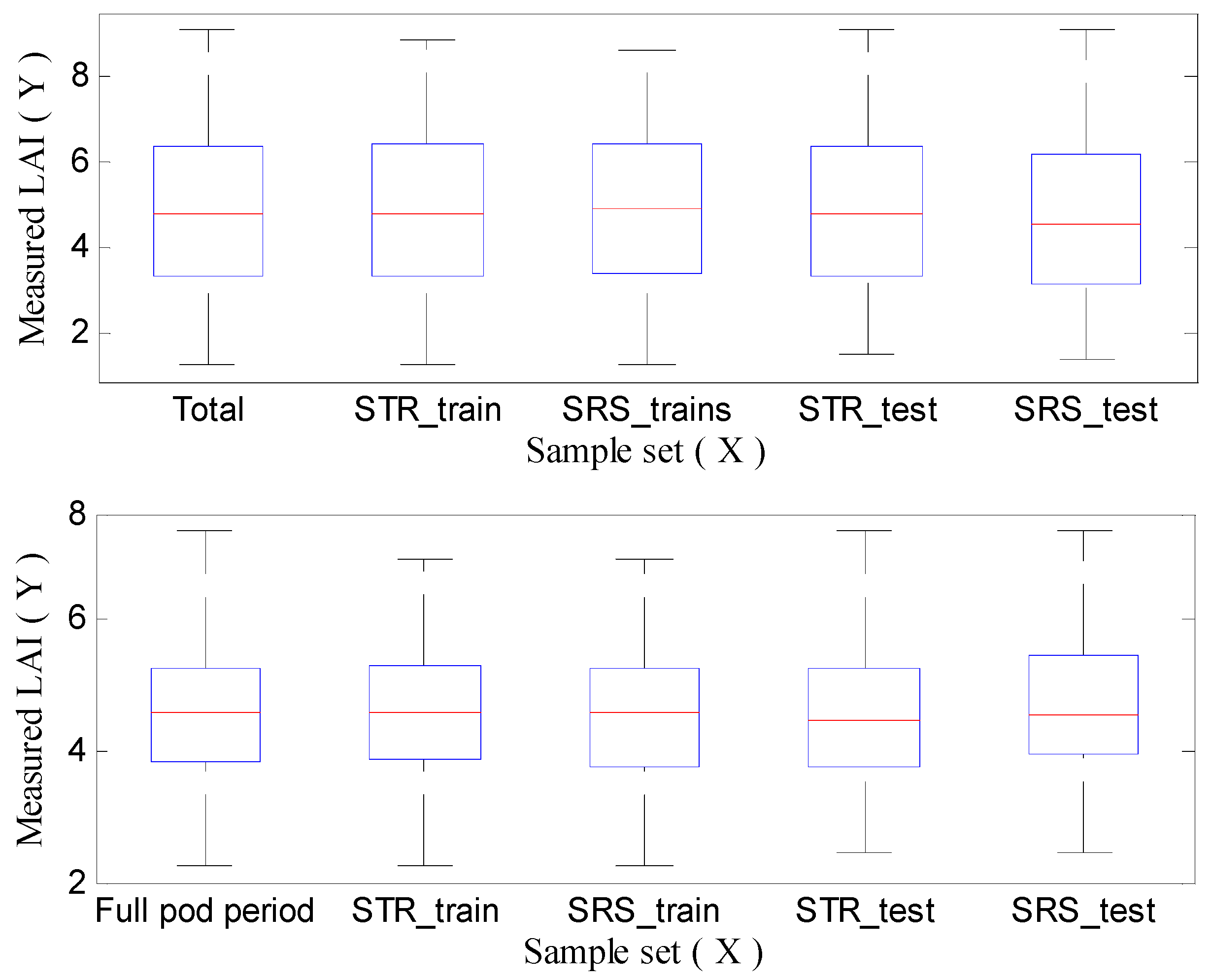
3.1. Calibration Set and Validation Set Based on Sampling Strategy

SRS and STR sampling strategies were used to classify all samples into calibration and validation sets. Over the whole growth period, the number of modeling samples was 400, and the number of validation samples was 143; the corresponding numbers for single growth periods were 92 and 31. Figure 3 shows the results of the set.seed (0) for SRS and STR in the statistical software package R 3.2.0. Boxplots for the population set, calibration set, and verification sample set based on STR were similar for the whole growth and single growth periods. The boxplot for the calibration set acquired by SRS similar to that for the population set, but the boxplot for the validation set was slightly different. Calibration sets aquired by the two sampling methods and the verification set based on STR were close to the distribution of the population set, indicating that the stratified sampling method was more reasonable.

3.2. Appropriate Model Parameters for LAI Inversion Model

Model construction and verification were carried out using R 3.2.0 software. The RF regression model references parameters reported in previous literature [23,32], and the tree number was set to 500 for the whole and single growth periods. The ANN regression model used a training subset and multiple iterations to derive the appropriate parameters [32]. The “tune.svm” function in R3.2.0 was used to find the optimal parameters for the SVM regression model [11,23]. Suitable principal components for the PLS model were chosen based on the variance explained by the independent variable. The optimal number of principal components was 5, and the cumulative rate of variables was 94% for the whole growth period; the optimal number of principal components and cumulative rate of variables were 5 and 80% for the single growth period [32]. The parameters of the final model after parameter optimization and multiple training are shown in Table 2.

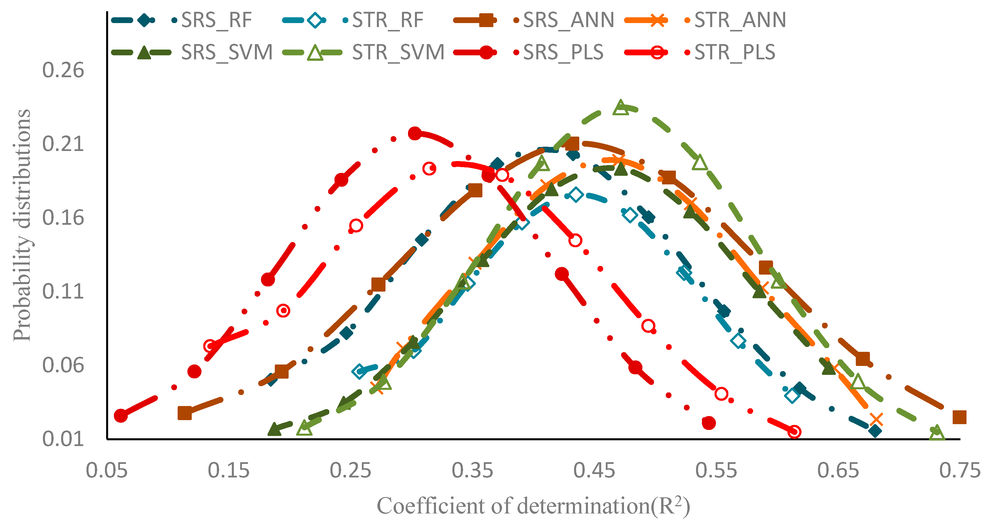
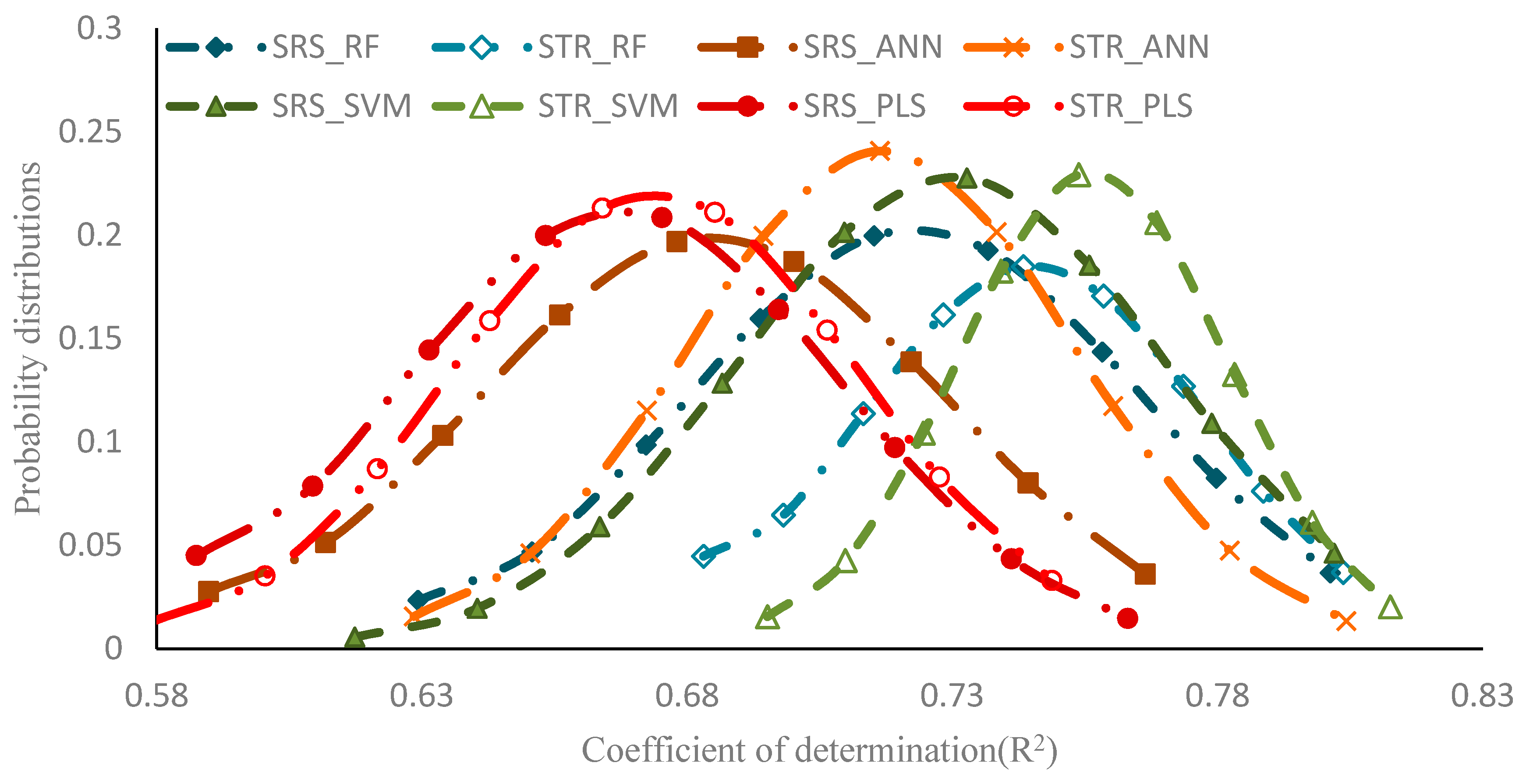
3.3. Comparison of Whole Growth Period Models

The validation accuracy (R2) of the regression models is shown in Figure 4 and Table 3. The regression models based on both sampling methods were tested for significance (p < 0.01). Compared to the non-parametric regression methods, the PLS model had similar R2 range of values for both SRS and STR methods (0.173 and 0.171, respectively). In contrast, the SPS and STR methods produced largely different results for the RF, SVM, and ANN models. The R2 values for the RF and SVM models based on SRS were significantly lower than the values for these models based on STR.
The STR method somewhat improved model performance (Table 3). The SVM method based on STR exhibited the lowest SDR2 (0.025), RMSE (0.104), and SDRMSE (0.005), and the highest R2 (0.749). The RF method based on STR was nearly as good, with R2 of 0.741, SDR2 of 0.031, RMSE of 0.106, and SDRMSE of 0.005, indicating an obvious improvement compared to the RF model based on SRS. Although PLS based on STR performed satisfactorily (R2 of 0.689, SDR2 of 0.033, RMSE of 0.114, and SDRMSE of 0.006), this model exhibited the poorest performance. The STR sampling method increased the precision (R2) and stability (SDR2 and SDRMSE) of the three regression models and the linear model (PLS) by varying degrees. Both the SVM and RF regression methods showed high precision in LAI estimation. The ANN model performed relatively poorly but still exhibited higher precision compared with the linear model. Based on SDRMSE, the STR method slightly increased the stability of model accuracy.

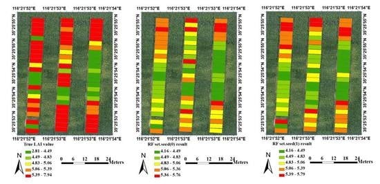
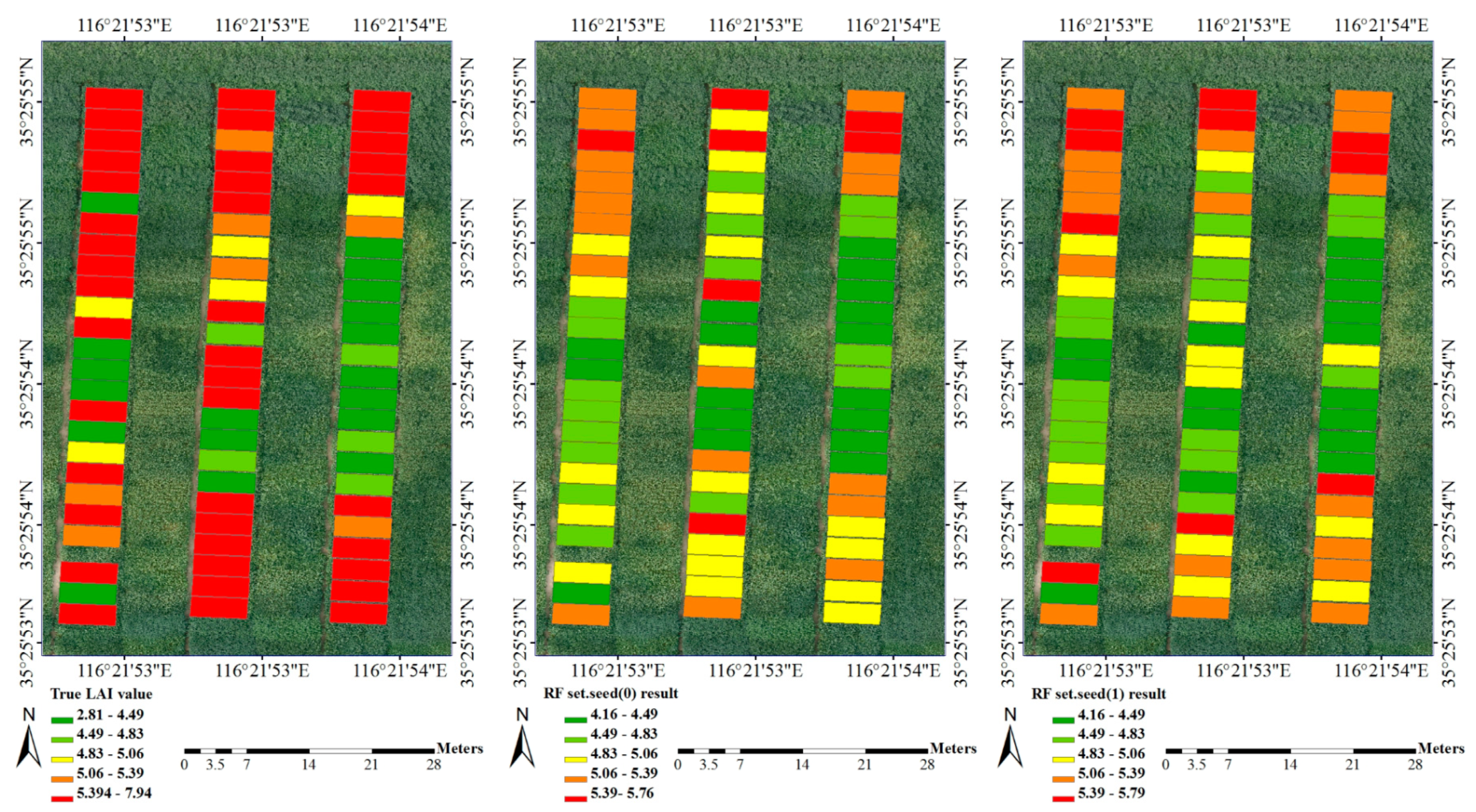
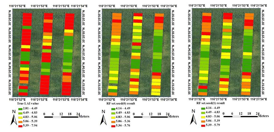
3.4. Comparison of Single Growth Period Models

The LAI values predicted using RF, SVM, ANN, and PLS for a single growth period (R4~R5 growth period) are shown in Figure 5 and Table 4. The difference between the maximum and minimum R2 of the PLS model based on SRS and STR was 0.482 and 0.480, respectively. The minimum R2 of the PLS model based on STR was higher than that of the SRS-based PLS model. The R2 values for the RF, SVM, and ANN models based on STR were similar, but not all R2 values were significant. R2 values for models based on the STR method were higher than values for models based on the SRS method to some extent, but the minimum R2 (0.235) of the ANN model was larger than that of other models.
Table 4 presents an evaluation of model performance for the single growth period (full pod period). ANN had the highest R2 and lowest RMSE for both the STR and SRS methods. The SDR2, RMSE, and SDRMSE values were lower and the R2 was higher for the ANN model based on the STR method compared with the SRS-based model. The STR sampling method remarkably improved the stability of both the non-parametric regression (i.e., RF, ANN, and SVM) and linear (i.e., PLS) models. The ANN model exhibited the highest accuracy, precision, and stability, whereas the RF model had the lowest precision, accuracy, and stability. However, the RF model performed better than the linear PLS model. Therefore, the ANN model was the most suitable for LAI inversion during a single growth period.

4. Discussion

The precision and stability of the LAI inversion model based on STR sampling were higher compared with those values for models based on SRS sampling for the whole and single growth periods (Table 3 and Table 4). The linear PLS estimation model also exhibited the same trend. The RF model was most suitable for LAI estimation during the whole growth period, and the ANN model was most appropriate for LAI estimation for a single growth period.
The maximum V-R2 values for the two LAI estimation models were approximately the same, but the minimum values were different (Figure 4 and Figure 5). The V-R2 values for models based on STR were more stable compared with values for SRS-based models because the RF, SVM, and ANN methods use sample feature dimensions to obtain prediction results. The stronger the representation of the samples, the stronger the generalization ability of the trained model (universal). The STR method can ensure that samples are sufficiently representative and reduce the complexity of learning [21]. From the principle of probability sampling (SRS and STR), we can see that the same set of data produced different calibration sets and predicted values. As shown in Figure 6, STR ensured that the calibration and verification sets were close to the distribution of the population set, although the prediction accuracy was variable. To avoid the effect of the model calibration set on model evaluation, we compared the average predicted results of the RF, SVM, ANN, and PLS models rather than case-specific results. STR reduced the probability of case-specific results to a certain extent and enhanced model transferability.
The selection of training samples by the two sampling methods varied slightly. The average and median values of training samples selected based on SRS deviated from the mean and median of the population samples. However, the distributions of training samples selected by STR were closer to the overall sample distribution. Results for the whole and single growth periods based on the two sampling strategies showed that the calibration set sampled based on STR for the whole growth period was significantly better than the SRS-extracted sample. Two factors affected the sampling method results: the sampling method and total sample distribution. SRS is a random sampling method, and the probability of becoming part of the training sample was the same for each sample in the population. STR divided samples into several layers using random sampling and, thus, could avoid the effect of small sample size, resulting in a sample distribution similar to the population distribution [30]. When collecting LAI data for the same growth period of the same soybean variety, the calibration set obtained by SRS was close to uniform distribution. The distribution of collected LAI data for different soybean varieties in each growth period was not balanced, which is consistent with results of previous studies [27]. To overcome the influence of growth period and soybean variety on model comparison, previous studies have compared model performance for single or whole growth periods of the same crop variety [23]. Most sampling methods cannot be sampled independently and must be used in conjunction with the model. We adopted STR sampling independently to avoid the above-mentioned factors [21,30].
One hundred repetitive extraction model calibration sets were used for LAI estimation, and models were evaluated based on the average of 100 results. The SVM and RF models were more accurate for the whole growth period, whereas the ANN model had the lowest accuracy (Table 3 and Table 4). However, the accuracy of the ANN model was higher for the single growth period, and that for the RF model was the lowest. ANN models can approximate complex nonlinear relationships sufficiently; however, when the data distribution is highly dispersed, the neural network model requires more parameters, which influences the generalization ability and credibility of the results [54]. The performance of the RF model was lower compared with the ANN and SVM models for the single growth period. Previous studies on SVM and RF model comparison have reported contrasting results [23], possibly due to use of only a single plant strain and one calibration set. The RF model is based on a large sample decision tree for high-dimensional data training and, thus, has a strong tolerance for data faults [39]. However, it is difficult to effectively train RF models with a small sample size [55]. The SVM model can avoid the effects of small sample size and high dimensionality as well as neural network structure selection and local optimization problems [46]. Based on our results, the RF model is suitable for estimating LAI over the whole growth period, and ANN is appropriate for estimations made over a single growth period. The SVM model exhibited high accuracy and stability over both the whole growth period and the single stage, which is consistent with previous studies [17].

5. Conclusions

Models were constructed using datasets obtained from SRS and STR sampling methods during the whole growth period and a single growth period to determine the optimal model for soybean (multiple strains) LAI inversion. RF, ANN, and SVM models were compared with a PLS model based on V-R2, SDR2, V-RMSE, and SDRMSE. The V-R2 values of the RF, ANN, and SVM estimation models for a single growth period were lower than the corresponding values for the whole growth period. The RF model, which is the optimal model for the whole growth period, could accurately (V-R2 = 0.741; V-RMSE = 0.106) and stably (SDR2 = 0.031; SDRMSE = 0.005) predict LAI for the whole growth period. The ANN model obtained more accurate (V-R2 = 0.452; V-RMSE = 0.086) and stable (SDR2 = 0.132 and SDRMSE = 0.009) estimation results than the RF model for a single growth period. The STR sampling method was superior to the SRS sampling method, and models based on this method performed equally well for LAI estimations over the whole and single growth periods. The ANN model produced the best estimation for the single growth period in which sample plots and sample variation were relatively low. The RF model was best for LAI estimations made over the whole growth period in which sample plots and sample variation were relatively large.

Acknowledgments

This study was supported by the Natural Science Foundation of China (61661136003, 41471285, 41471351), the National Key Research and Development Program (2016YFD0300602), the Special Funds for Technology innovation capacity building sponsored by the Beijing Academy of Agriculture and Forestry Sciences (KJCX20170423), and the UK Science and Technology Facilities Council through the PAFiC project (Ref: ST/N006801/1). Thanks to Guozheng Lu, Jibo Yue, etc., in the field sampling collection. Thanks to all employees of Shandong Shengfeng soybean breeding group. We are grateful to the anonymous reviewers for their valuable comments and recommendations.

Author Contributions

Huanhuan Yuan, Guijun Yang, and Jiangang Liu analyzed the data and wrote the manuscript; Changchun Li, Yanjie Wang, Haiyang Yu, Haikuan Feng, Bo Xu, and Xiaoqing Zhao provided comments and suggestions for the manuscript and checked the writing; Xiaodong Yang provided data and data acquisition capacity.

Conflicts of Interest

The authors declare no conflict of interest.

References

  1. Lugg, D.G.; Sinclair, T.R. Seasonal changes in photosynthesis of field-grown soybean leaflets. 2. Relation to nitrogen content. Photosynthetica 1981, 15, 138–144. [Google Scholar]
  2. Burkey, K.O.; Wells, R. Response of soybean photosynthesis and chloroplast membrane function to canopy development and mutual shading. Plant Physiol. 1991, 97, 245–252. [Google Scholar] [CrossRef] [PubMed]
  3. Boerma, H.R.; Specht, J.E. Soybeans: Improvement, Production and Uses; American Society of Agronomy: Madison, WI, USA, 2004. [Google Scholar]
  4. Chen, J.M.; Pavlic, G.; Brown, L.; Cihlar, J.; Leblanc, S.G. Derivation and validation of Canada-wide coarse-resolution leaf area index maps using high-resolution satellite imagery and ground measurements. Remote Sens. Environ. 2002, 80, 165–184. [Google Scholar] [CrossRef]
  5. Running, S.W.; Nemani, R.R.; Heinsch, F.A.; Zhao, M.; Reeves, M. A continuous satellite-derived measure of global terrestrial primary production. Bioscience 2004, 54, 547–560. [Google Scholar] [CrossRef]
  6. Breda, N. Ground-based measurements of leaf area index: A review of methods, instruments and current controversies. J. Exp. Bot. 2003, 54, 2403–2417. [Google Scholar] [CrossRef] [PubMed]
  7. Jonckheere, I.; Fleck, S.; Nackaerts, K.; Muys, B.; Coppin, P.; Weiss, M.; Baret, F. Review of methods for in situ leaf area index determination—Part I. Theories, sensors and hemispherical photography. Agric. For. Meteorol. 2004, 121, 19–35. [Google Scholar] [CrossRef]
  8. Campos-Taberner, M.; Javier Garcia-Haro, F.; Camps-Valls, G.; Grau-Muedra, G.; Nutini, F.; Crema, A.; Boschetti, M. Multitemporal and multiresolution leaf area index retrieval for operational local rice crop monitoring. Remote Sens. Environ. 2016, 187, 102–118. [Google Scholar] [CrossRef]
  9. Liu, K.; Zhou, Q.; Wu, W.; Xia, T.; Tang, H. Estimating the crop leaf area index using hyperspectral remote sensing. J. Integr. Agric. 2016, 15, 475–491. [Google Scholar] [CrossRef]
  10. Li, X.; Zhang, Y.; Bao, Y.; Luo, J.; Jin, X.; Xu, X.; Song, X.; Yang, G. Exploring the best hyperspectral features for LAI estimation using partial least squares regression. Remote Sens. 2014, 6, 6221–6241. [Google Scholar] [CrossRef]
  11. Liang, L.; Di, L.; Zhang, L.; Deng, M.; Qin, Z.; Zhao, S.; Lin, H. Estimation of crop LAI using hyperspectral vegetation indices and a hybrid inversion method. Remote Sens. Environ. 2015, 165, 123–134. [Google Scholar] [CrossRef]
  12. Fan, W.J.; Xu, X.R.; Liu, X.C.; Yan, B.Y.; Cui, Y.K. Accurate LAI retrieval method based on PROBA/CHRIS data. Hydrol. Earth Syst. Sci. 2010, 14, 1499–1507. [Google Scholar] [CrossRef]
  13. Delegido, J.; Verrelst, J.; Rivera, J.P.; Ruiz-Verdu, A.; Moreno, J. Brown and green LAI mapping through spectral indices. Int. J. Appl. Earth Obs. 2015, 35, 350–358. [Google Scholar] [CrossRef]
  14. Vuolo, F.; Dini, L.; D’Urso, G. Retrieval of leaf area index from CHRIS/PROBA data: An analysis of the directional and spectral information content. Int. J. Remote Sens. 2008, 29, 5063–5072. [Google Scholar] [CrossRef]
  15. Jihua, M.; Bingfang, W.; Qiangzi, L. Method for estimating crop leaf area index of China using remote sensing. Trans. Chin. Soc. Agric. Eng. 2007, 23, 160–167. [Google Scholar]
  16. Verrelst, J.; Camps-Valls, G.; Munoz-Mari, J.; Pablo Rivera, J.; Veroustraete, F.; Clevers, J.G.P.W.; Moreno, J. Optical remote sensing and the retrieval of terrestrial vegetation bio-geophysical properties—A review. ISPRS J. Photogramm. Remote Sens. 2015, 108, 273–290. [Google Scholar] [CrossRef]
  17. Liang, D.; Guan, Q.; Huang, W.; Huang, L.; Yang, G. Remote sensing inversion of leaf area index based on support vector machine regression in winter wheat. Trans. Chin. Soc. Agric. Eng. 2013, 29, 117–123. [Google Scholar]
  18. Meroni, M.; Colombo, R.; Panigada, C. Inversion of a radiative transfer model with hyperspectral observations for LAI mapping in poplar plantations. Remote Sens. Environ. 2004, 92, 195–206. [Google Scholar] [CrossRef]
  19. Duan, S.; Li, Z.; Wu, H.; Tang, B.; Ma, L.; Zhao, E.; Li, C. Inversion of the PROSAIL model to estimate leaf area index of maize, potato, and sunflower fields from unmanned aerial vehicle hyperspectral data. Int. J. Appl. Earth Obs. 2014, 26, 12–20. [Google Scholar] [CrossRef]
  20. Herrmann, I.; Pimstein, A.; Karnieli, A.; Cohen, Y.; Alchanatis, V.; Bonfil, D.J. LAI assessment of wheat and potato crops by VENμS and Sentinel-2 bands. Remote Sens. Environ. 2011, 115, 2141–2151. [Google Scholar] [CrossRef]
  21. Megainduction, J.C. Machine Leaming on Very Large Database; School of Computer Science, University of Technology: Sydney, Australia, 1991. [Google Scholar]
  22. Darvishzadeh, R.; Skidmore, A.; Schlerf, M.; Atzberger, C.; Corsi, F.; Cho, M. LAI and chlorophyll estimation for a heterogeneous grassland using hyperspectral measurements. ISPRS J. Photogramm. Remote Sens. 2008, 63, 409–426. [Google Scholar] [CrossRef]
  23. Han, Z.Y.; Zhu, X.C.; Fang, X.Y.; Wang, Z.Y.; Wang, L.; Zhao, G.X.; Jiang, Y.M. Hyperspectral estimation of apple tree canopy LAI based on SVM and RF regression. Spectrosc. Spectr. Anal. 2016, 36, 800–805. [Google Scholar]
  24. Omer, G.; Mutanga, O.; Abdel-Rahman, E.M.; Adam, E. Empirical prediction of Leaf Area Index (LAI) of endangered tree species in intact and fragmented indigenous forests Ecosystems using WorldView-2 data and two robust machine learning algorithms. Remote Sens. 2016, 8, 324. [Google Scholar] [CrossRef]
  25. Verrelst, J.; Munoz, J.; Alonso, L.; Delegido, J.; Pablo Rivera, J.; Camps-Valls, G.; Moreno, J. Machine learning regression algorithms for biophysical parameter retrieval: Opportunities for Sentinel-2 and -3. Remote Sens. Environ. 2012, 118, 127–139. [Google Scholar] [CrossRef]
  26. Mustafa, Y.T.; Van Laake, P.E.; Stein, A. Bayesian network modeling for improving forest growth estimates. IEEE Trans. Geosci. Remote 2011, 49, 639–649. [Google Scholar] [CrossRef]
  27. Bo, Q.I.; Zhang, N.; Zhao, T.J.; Xing, G.N.; Zhao, J.M.; Gai, J.Y. Prediction of leaf area index using hyperspectral remote sensing in breeding programs of soybean. Acta Agron. Sin. 2015, 41, 1073. [Google Scholar]
  28. Wong, T. Parametric methods for comparing the performance of two classification algorithms evaluated by k-fold cross validation on multiple data sets. Pattern Recogn. 2017, 65, 97–107. [Google Scholar] [CrossRef]
  29. Mingliang, L.I.; Yang, D.; Chen, J. Probabilistic flood forecasting by a sampling-based Bayesian model. J. Hydroelectr. Eng. 2011, 30, 27–33. [Google Scholar]
  30. Cochran, W.G. Sampling Technique; China Statistical Publishing House: Beijing, China, 1985. [Google Scholar]
  31. Aasen, H.; Burkart, A.; Bolten, A.; Bareth, G. Generating 3D hyperspectral information with lightweight UAV snapshot cameras for vegetation monitoring: From camera calibration to quality assurance. ISPRS J. Photogramm. 2015, 108, 245–259. [Google Scholar] [CrossRef]
  32. Li, Z.; Wang, J.; Tang, H.; Huang, C.; Yang, F.; Chen, B.; Wang, X.; Xin, X.; Ge, Y. Predicting grassland leaf area index in the Meadow Steppes of Northern China: A comparative study of regression approaches and hybrid geostatistical methods. Remote Sens. 2016, 8, 632. [Google Scholar] [CrossRef]
  33. Wang, J.; Zhao, C.; Huang, W. Foundations and Applications of Quantitative Remote Sensing in Agriculture, 1st ed.; Science Press: Beijing, China, 2008; pp. 156–157. [Google Scholar]
  34. Demetriades-Shah, T.H.; Steven, M.D.; Clark, J.A. High resolution derivative spectra in remote sensing. Remote Sens. Environ. 1990, 33, 55–64. [Google Scholar] [CrossRef]
  35. Frigge, M.; Hoaglin, D.C.; Iglewicz, B. Some implementations of the boxplot. Am. Stat. 1989, 43, 50–54. [Google Scholar] [CrossRef]
  36. Benjamini, Y. Opening the box of a boxplot. Am. Stat. 1988, 42, 257–262. [Google Scholar] [CrossRef]
  37. Cheng, T.; Riaño, D.; Koltunov, A.; Whiting, M.L.; Ustin, S.L.; Rodriguez, J. Detection of diurnal variation in orchard canopy water content using MODIS/ASTER Airborne Simulator (MASTER) data. Remote Sens. Environ. 2013, 132, 1–12. [Google Scholar] [CrossRef]
  38. Sandelowski, M. Sample size in qualitative research. Res. Nurs. Health 1995, 18, 179–183. [Google Scholar] [CrossRef] [PubMed]
  39. Breiman, L. Random forests. Mach. Learn. 2001, 45, 5–32. [Google Scholar] [CrossRef]
  40. Krishnan, P.; Alexander, J.D.; Butler, B.J.; Hummel, J.W. Reflectance technique for predicting soil organic matter. Soil Sci. Soc. Am. J. 1980, 44, 1282–1285. [Google Scholar] [CrossRef]
  41. Liaw, A.; Wiener, M. Classification and regression by randomForest. R News 2002, 2, 18–22. [Google Scholar]
  42. He, Q. Neural Network and its Application in IR; Graduate School of Library and Information Science, University of Illinois at Urbana-Champaign Spring: Champaign, IL, USA, 1999. [Google Scholar]
  43. Kimes, D.S.; Nelson, R.F.; Manry, M.T.; Fung, A.K. Review article: Attributes of neural networks for extracting continuous vegetation variables from optical and radar measurements. Int. J. Remote Sens. 1998, 19, 2639–2663. [Google Scholar] [CrossRef]
  44. R Core Team. R: A Language and Environment for Statistical Computing; R Foundation for Statistical Computing: Vienna, Austria, 2011. [Google Scholar]
  45. Cortes, C.; Vapnik, V. Support-vector networks. Mach. Learn. 1995, 20, 273–297. [Google Scholar] [CrossRef]
  46. Vapnik, V.N.; Vapnik, V. Statistical Learning Theory; Wiley: New York, NY, USA, 1998; Volume 1. [Google Scholar]
  47. Si, W.; Amari, S.I. Conformal transformation of Kernel functions: A data-dependent way to improve support vector machine classifiers. Neural Process. Lett. 2002, 15, 59–67. [Google Scholar]
  48. Dimitriadou, E.; Hornik, K.; Leisch, F.; Meyer, D.; Weingessel, A. The R Project for Statistical Computing. Available online: http://www.r-project.org (accessed on 6 April 2005).
  49. Geladi, P.; Kowalski, B.R. Partial least-squares regression: A tutorial. Anal. Chim. Acta 1986, 185, 1–17. [Google Scholar] [CrossRef]
  50. Geisser, S. A predictive approach to the random effect model. Biometrika 1974, 61, 101–107. [Google Scholar] [CrossRef]
  51. Wolter, P.T.; Townsend, P.A.; Sturtevant, B.R.; Kingdon, C.C. Remote sensing of the distribution and abundance of host species for spruce budworm in Northern Minnesota and Ontario. Remote Sens. Environ. 2008, 112, 3971–3982. [Google Scholar] [CrossRef]
  52. Mevik, B.; Wehrens, R. The pls package: Principal component and partial least squares regression in R. J. Stat. Softw. 2007, 18, 1–24. [Google Scholar] [CrossRef]
  53. Tedeschi, L.O. Assessment of the adequacy of mathematical models. Agric. Syst. 2006, 89, 225–247. [Google Scholar] [CrossRef]
  54. Tu, J.V. Advantages and disadvantages of using artificial neural networks versus logistic regression for predicting medical outcomes. J. Clin. Epidemiol. 1996, 49, 1225–1231. [Google Scholar] [CrossRef]
  55. Deng, H.; Runger, G.; Tuv, E. Bias of importance measures for multi-valued attributes and solutions. In Proceedings of the International Conference on Artificial Neural Networks, Espoo, Finland, 14–17 June 2011; pp. 293–300. [Google Scholar]
Figure 1. Distribution of the sampling sites in Shandong Jiaxiang. Each plot is a 3 × 5 m rectangle with six rows of crops 5 m in length, and each row gap is 0.5 m. The average spectrum of SCA1001 plot acquired from the snapshot imaging hyperspectral spectrometer.
Remotesensing 09 00309 g001
Figure 2. Flowchart of the methodology. Two sampling strategies were used separately to obtain 100 calibration sets. RF, ANN, SVM, and PLS models were used to generate 100 V-R2 and V-RMSE.
Remotesensing 09 00309 g002
Figure 3. Statistics of population set, calibration set, and validation set. STR_train represents the calibration set acquired by stratified sampling; STR_test represent the validation set acquired by stratified sampling; SRS_train represents the calibration set acquired by simple random sampling; STR_test represents the validation set acquired by simple random sampling.
Remotesensing 09 00309 g003
Figure 4. Distribution of the V-R2 of different models and sampling strategies in whole growth period.
Remotesensing 09 00309 g004
Figure 5. Distribution of the V-R2 of different models and sampling strategies in single growth period.
Remotesensing 09 00309 g005
Figure 6. Prediction result of RF model with two different calibration sets.
Remotesensing 09 00309 g006
Table 1. Statistical description of soybean LAI. p value is the result of Kolmogorov-Smirnov test.
Growing PeriodObservation PlotsMax ValueMin ValueMean Valuep ValueCoefficient of Variation
R1 period965.7051.2852.9880.0000.331
R3 period1269.065.4157.2950.051 *0.116
R5 period1238.223.155.4790.0020.197
R6 period1166.541.834.240.192 *0.262
R7 period826.781.5853.5790.0000.345
R1~R7 period5439.061.2854.9060.0000.382
Note: * indicates that the observed LAI is uniformly distributed.
Table 2. Parameters of regression models.
RF Regression Model Parameters
Growth PeriodNtreemtryNorm.votesReference
whole growth period5002TRUELiang et al. [11]
single growth period5002TRUE
ANN Regression Model Parameters
WeightSizeDecayMaxitSwitch for entropy
whole growth period110.0011000Least squaresLi et al. [32]
single growth period110.00051000Least squares
SVM Regression Model Parameters
ShrinkingGammaEpsCkernelProbability
whole growth period10.0010.011radial basis1Li et al. [32]
single growth period10.010.011radial basis1
PLS Regression Model Parameters
NcompValidation
whole growth period5cross-validation (CV)Li et al. [32]
single growth period5cross-validation (CV)
Table 3. Different model performances in the prediction of whole period soybean LAI.
Regression MethodV-R2V-RMSE
R2SDR2RMSESDRMSE
SRSRF0.7120.0420.1060.007
ANN0.6740.0440.110.006
SVM0.7180.0400.1020.006
PLS0.6570.0410.1140.006
STRRF0.7410.0310.1060.005
ANN0.7060.0360.110.006
SVM0.7490.0250.1040.005
PLS0.6890.0330.1140.006
Table 4. Different model performances in the prediction of single period soybean LAI.
Regression MethodV-R2V-RMSE
R2SDR2RMSESDRMSE
SRSRF0.3750.1370.0900.009
ANN0.4270.1350.0860.010
SVM0.4080.1300.0880.010
PLS0.2740.1090.1040.012
STRRF0.4000.1300.0880.009
ANN0.4520.1320.0860.009
SVM0.4390.1080.0890.007
PLS0.3090.1200.1020.011

