
Multi-Feature Segmentation for High-Resolution Polarimetric SAR Data Based on Fractal Net Evolution Approach


Faculty of Information Engineering, China University of Geosciences (Wuhan), Wuhan 430074, China
*
Author to whom correspondence should be addressed.
Remote Sens. 2017, 9(6), 570; https://doi.org/10.3390/rs9060570
Submission received: 24 February 2017
/
Revised: 23 May 2017
/
Accepted: 4 June 2017
/
Published: 6 June 2017
(This article belongs to the Special Issue Advances in SAR: Sensors, Methodologies, and Applications)
Abstract
:Segmentation techniques play an important role in understanding high-resolution polarimetric synthetic aperture radar (PolSAR) images. PolSAR image segmentation is widely used as a preprocessing step for subsequent classification, scene interpretation and extraction of surface parameters. However, speckle noise and rich spatial features of heterogeneous regions lead to blurred boundaries of high-resolution PolSAR image segmentation. A novel segmentation algorithm is proposed in this study in order to address the problem and to obtain accurate and precise segmentation results. This method integrates statistical features into a fractal net evolution algorithm (FNEA) framework, and incorporates polarimetric features into a simple linear iterative clustering (SLIC) superpixel generation algorithm. First, spectral heterogeneity in the traditional FNEA is substituted by the G0 distribution statistical heterogeneity in order to combine the shape and statistical features of PolSAR data. The statistical heterogeneity between two adjacent image objects is measured using a log likelihood function. Second, a modified SLIC algorithm is utilized to generate compact superpixels as the initial samples for the G0 statistical model, which substitutes the polarimetric distance of the Pauli RGB composition for the CIELAB color distance. The segmentation results were obtained by weighting the G0 statistical feature and the shape features, based on the FNEA framework. The validity and applicability of the proposed method was verified with extensive experiments on simulated data and three real-world high-resolution PolSAR images from airborne multi-look ESAR, spaceborne single-look RADARSAT-2, and multi-look TerraSAR-X data sets. The experimental results indicate that the proposed method obtains more accurate and precise segmentation results than the other methods for high-resolution PolSAR images.

1. Introduction
1.1. Background
Synthetic aperture radar (SAR) has been widely accepted as an indispensable method for Earth monitoring due to its all-day/all-weather capacity and penetration capability [1,2,3,4]. Fully polarimetric SAR (PolSAR) emits or receives two orthogonal polarized radar waves, and allows the discrimination of different scattering mechanisms. PolSAR image segmentation is able to obtain distinct and self-similar pixel groups that depict homogeneous regions, with virtually no speckle noise [5]. Since accurate segmentation is important for subsequent classification and extraction of surface parameters [6,7], PolSAR image segmentation has been increasingly used for land use and land cover classification [8], land development detection [9], and oil seep detection [10].
With a new generation of advanced SAR sensors, higher-resolution PolSAR images of the Earth’s surface have been acquired. In addition to being affected by speckle, the high-resolution PolSAR images show the following characteristics:
- (1)
- Spatial characteristics: The decrease in the resolution cell provides richer spatial details of ground objects [11], such as significant geometric shape features and texture information.
- (2)
- Statistical characteristics: The scattering vectors from the homogeneous regions of medium- or low-resolution PolSAR data can be modeled using Gaussian distributions. The corresponding coherency matrices have a complex Wishart distribution [12]. However, in high-resolution PolSAR data, a significantly reduced number of sub-scatterers within a resolution cell leads to a greater heterogeneity [13], particularly in urban areas, where clusters can no longer be modeled using a Gaussian process.
In short, high-resolution PolSAR images usually contain speckle noise, and many heterogeneous regions, with rich spatial features. The complexity makes segmentation of high-resolution PolSAR images a very challenging task. In this paper, research on segmentation for high-resolution PolSAR images is reported.
1.2. Related Work
Some classic segmentation algorithms for PolSAR images have been proposed, including the Markov random field (MRF) [14,15], statistical region merging (SRM) [5], hierarchical segmentation [16,17], and superpixel segmentation [18,19,20]. Liu et al. [15] proposed a spatially adaptive segmentation method to keep each segment at an appropriate size and shape based on multiscale wedgelet analyses and Wishart MRF (MW-WMRF). Lang et al. [5] utilized the generalized statistical region merging (GSRM) algorithm, based on the product model, which shows improved robustness and anti-noise performance without any assumption on PolSAR data distributions. Alonso-González et al. [17] used binary partition trees (BPT) to develop a novel region-based and multi-scale PolSAR data representation for speckle noise filtering and segmentation, on the basis of the Gaussian hypothesis. Liu et al. [18] oversegmented PolSAR images into many local and coherent regions using the normalized cuts algorithm to improve the classification accuracy by adding inherent statistical characteristics to the contour information. Ersahin et al. [21] segmented PolSAR data with contour information and spatial proximity, based on spectral graph partitioning for object oriented classification. In summary, an increasing number of methods are combining spatial features and statistical properties of PolSAR images to obtain useful segmentation results.
Segmentation using spatial features is a common method to model a labeling process as MRF [14,15], which includes the spatial relationships between pixels. In contrast, the fractal net evolution algorithm (FNEA) makes good use of the geometric shape features and spectral information of targets [22]. This was successfully used in high spatial resolution, optical image segmentation [23,24]. FNEA is a bottom-up region merging technique with a fractal iterative heuristic optimization procedure. It starts with a single pixel and a pairwise comparison of its neighbors, with the aim of minimizing the resulting merged heterogeneity. The heterogeneity is determined using geometric shapes and the standard deviation of spectral properties as its basis. By replacing spectral information with the parameters of H/α/A decomposition [25], Freeman decomposition [26], or Pauli decomposition [8,9], researchers have introduced FNEA into PolSAR image segmentation for object-oriented classification. Benz and Pottier [25] first used FNEA to segment filtered PolSAR images by employing shape features, H/α/A, and the total scattered power span. Qi et al. [8] implemented FNEA segmentation on a Pauli RGB composition image of filtered PolSAR data, and successfully applied it to land-use and land-cover classification. However, the segmentation results of these methods were easily influenced by speckle noise, and the results were too fragmented to represent unbroken land parcels [8] as the statistical characteristics of PolSAR data were not used.
Segmentation, using statistical features uses the classical complex Wishart distribution, which has been widely used with PolSAR data [15,17,19,20,21,27]. As the Gaussian or Wishart model does not agree well with heterogeneous scenes of high-resolution images, heterogeneity is usually modeled as the product of the square root of a textured random variable and an independent, zero-mean, complex circular Gaussian speckle random vector [28]. If the random texture variable is Gamma, inverse Gamma, or Fisher distributed, the target coherency matrices follow multivariate K distribution [29], G0 distribution [30], or KummerU distribution [31], respectively. Beaulieu and Touzi [16] presented a hierarchical segmentation method using the K-distribution model, and verified its effectiveness for textured forested areas. Bombrun et al. [32] proposed a hierarchical maximum likelihood segmentation for high-resolution PolSAR images using KummerU distribution heterogeneous clutter models, which provided a better performance compared to the classical Gaussian criterion. However, it is essential to robustly estimate the parameters of these multiplicative models with enough samples. Generally, the segmentation results have obvious dentate boundaries, as the initial samples are usually collected from image blocks within square windows [32]. Moreover, the accuracy of parameter estimation decreases due to the differences between the square blocks and the actual boundaries of targets in high-resolution PolSAR data.
1.3. The Proposed Approach
Superpixel algorithms group pixels into meaningful atomic regions, which are roughly homogeneous in size and shape, and can be used to replace the rigid structure of the pixel grid or the square block. Since the utilization of superpixels helps to overcome the influence of speckle noise and to preserve statistical characteristics [19,33,34], it has gradually become an important preprocessing step for segmentation or classification. Recently, Achanta et al. proposed a new superpixel algorithm, simple linear iterative clustering (SLIC), which adapted a k-means clustering approach to efficiently generate superpixels [35]. Considering the simplicity, fast processing and excellent boundary adherence of SLIC, Qin et al. [19] introduced the superpixel algorithm into PolSAR image segmentation by combining it with the Wishart hypothesis test distance and the spatial distance.
We propose a novel segmentation algorithm for high-resolution PolSAR data by combining spatial, statistical, and polarimetric features; this algorithm integrates statistical features into a FNEA framework, and the polarimetric features with SLIC, in order to generate pre-segments. Given that the G0 distribution has been shown to be flexible, computationally inexpensive, and capable of modeling varying degrees of texture [30,36], we substitute the G0 distribution of statistical heterogeneity for the spectral heterogeneity in the traditional FNEA. Furthermore, we also utilize a modified SLIC algorithm to generate compact, approximately homogeneous superpixels as initial samples for the statistical model, which utilizes the polarimetric distance of Pauli RGB composition instead of the CIELAB color distance.
The remainder of this paper is organized as follows; Section 2 describes the proposed segmentation method for high-resolution PolSAR data. The employed PolSAR images and the experimental and evaluation results are reported in Section 3. The discussion of the results is presented in Section 4. Conclusions are given in Section 5.
2. Methodology
The proposed approach is based on the FNEA framework, and can be divided into three main parts: (1) a statistical heterogeneity measure using the G0 distribution model for high-resolution PolSAR data; (2) initial sample generation for the statistical model using the SLIC algorithm with polarimetric features; and (3) segmentation with the G0 statistical and shape features, based on the FNEA framework. The details of these are explained in subsequent subsections.
2.1. FNEA
FNEA merges two adjacent objects with a fractal iterative heuristic optimization procedure, which starts with single-pixel objects, and satisfies the condition of minimizing the resulting merged heterogeneity [22,23].
The heterogeneity between two adjacent image objects is defined by integrating the change of spectral heterogeneity with the change of shape heterogeneity in a virtual merge [22], as follows:
where is the weight of the shape feature, and . Adjacent objects i and j are merged when the smallest growth in heterogeneity occurs.
For multispectral remote sensing images, can be described by adding weight to image channels c [22],
where n denotes the objects size, which is the number of pixels in an image object; and denotes the spectral heterogeneity of the image object, which is the standard deviation within the objects of channel c.
The change of shape heterogeneity can be expressed as
where denotes the shape heterogeneity of the image object, which is described with regard to smoothness and compactness. It is described by
where is the weight of smoothness, and . The smoothness heterogeneity is defined as the ratio of factual edge length p and border length b; b is given by the bounding box of an image object parallel to the raster while the compactness heterogeneity is defined as the ratio of factual edge length p and the square root of n [22].
At each iteration in FNEA, an image object is merged into its adjacent image object with the minimum heterogeneity, and when the heterogeneity is less than threshold t (i.e., scale parameter). If all increases exceed the scale parameter, no further merging occurs and the segmentation stops. The larger scale parameter t is, the more image objects can be merged and the larger the image objects grow.
2.2. Statistical Heterogeneity Measure by the G0 Model
PolSAR data are mainly provided in two forms: The single-look scattering matrix and the multi-look polarimetric coherency (or covariance) matrix. Each pixel of PolSAR data can be described by a 2 × 2 complex scattering matrix S [2]:
where H and V represent the horizontal and vertical polarization directions, respectively.
In a reciprocal medium, and S can be transformed into a three-dimensional single-look scattering vector using the complex Pauli spin matrix basis set [2,27]:
where denotes the matrix transpose. In this paper, the dimension of the scattering vector is denoted by d (d = 3 for the reciprocal case).
Usually, L-look coherency matrix T is computed to suppress speckle using the average of of the surrounding pixels, as follows [2,27]:
where is the conjugate transpose of scattering vector , and L is the number of looks.
2.2.1. G0 Model for High-Resolution PolSAR Data
High-resolution PolSAR images are greatly affected by heterogeneity due to the significantly reduced number of scatterers within a resolution cell [11]. The heterogeneity is usually modeled with the multiplicative models [28].
For single-look complex PolSAR data, the multiplicative model is given by
where is a texture random variable, and is a d-dimensional speckle vector, which follows an independent zero-mean multivariate complex Gaussian distribution.
Assume that in Equation (8) obeys the inverse Gamma distribution, in which the probability density function (PDF) is given by
where is the shape parameter and is the standard Euler Gamma function.
In this case, the target scattering vector k follows the G0 distribution, which is characterized by the following PDF [37]:
where is the covariance matrix of k, denotes the mathematical expectation, and represents the determinant, while denotes the inverse.
For multi-look PolSAR data, coherency matrix is modeled as the product of random variable τ and independent random matrix :
where obeys a Wishart distribution.
For an inverse gamma distributed texture, target coherency matrix follows the G0 distribution [30], which is characterized by the PDF, as follows:
where , is the trace operator and L is number of looks. represents the multivariate gamma function, defined as
2.2.2. Statistical Heterogeneity Measure
Since the log likelihood function can be used to measure the similarity between two segments in a hierarchical segmentation of PolSAR Images [16,32], it is utilized to measure the statistical heterogeneity between two image objects. At each iteration, merging two image objects using statistical features yields a decrease in the log likelihood function. Thus, the two adjacent image objects, i and j, should be merged to produce the smallest decrease of the log likelihood function. The change of statistical heterogeneity can be expressed as
where denotes the statistical heterogeneity of image object O, which is the maximum log likelihood value of the image object.
For single-look complex PolSAR data, the statistical heterogeneity of image object O is given by
where pixels in image object O are considered independent realizations, with respect to the assumed PDF in Equation (10).
According to Equations (10), (14), and (15), the statistical heterogeneity of image object O can be simplified to
where n is the number of pixels in image object O, , and are the best likelihood estimates of , and for this image object.
For multi-look PolSAR data, with respect to the assumed PDF in Equation (12), the statistical heterogeneity of image object O is
Similarly, the statistical heterogeneity of image object O can be simplified by Equations (12), (14), and (17) to
It can be concluded that the statistical heterogeneity from Equation (18) is equivalent to Equation (16) when L = 1, which means that the change in statistical heterogeneity can be computed by Equations (14) and (18), for both single-look and multi-look data.
2.2.3. Parameter Estimation
The number of looks, , is generally an integer provided by the SAR sensor. Statistical heterogeneity measured by the G0 distribution model is parameterized by scale matrix Σ and shape parameter α. The correct and reasonable merging objects are based on the proper estimation of the involved parameters.
Scale matrix is the mathematical expectation of the coherency matrix, which can be calculated using the classical sample covariance matrix estimator [38], as follows:
where denotes sample averaging, and N is the number of samples.
Shape parameter α can be estimated using the method of matrix log-cumulants, which has been proposed in the literature [39]. However, given that this method is more complex, needing a large amount of computation, and that this calculation is performed for each image object in each iteration of the segmentation, we estimate shape parameter α using the method of Doulgeris, provided in the literature [40]. This estimator is given by
where , and is the statistical variance.
2.3. Initial Samples Generation for Statistical Model
Accurate and robust parameter estimation of the statistical models requires sufficient samples. Since FNEA starts region merging from a single pixel, the number of samples (i.e., pixels in each image object) is too small to accurately estimate parameters at the beginning of the iterations. Generally, the image blocks within square windows are used as samples. However, there are obvious differences between the square blocks and the actual boundaries of targets in high-resolution PolSAR data. Therefore, in this work, the SLIC superpixel algorithm with polarimetric and spatial features was used to produce suitable initial samples before the utilization of statistical heterogeneity.
The SLIC algorithm incorporates k-means clustering to efficiently produce superpixels for images in the CIELAB color space [35]. It includes two main steps: Initializing m cluster centers and assigning each pixel to the nearest cluster center in a local search region. This algorithm has a speed advantage over traditional k-means clustering by limiting the size of the search area to reduce the number of distance calculations. In general, a key parameter, m, is the desired size of the superpixels, with approximately equal pixels [35].
Pauli RGB images can be obtained by using them as blue, red, and green channels, respectively. This has become the standard display mode of PolSAR data [41]. Hence, the polarimetric feature space of Pauli RGB composition was used to replace the CIELAB color space for the polarimetric SAR images.
The method of initial samples generation for statistical model using SLIC algorithm includes the following three main steps:
(1) Initializing cluster centers. The algorithm begins by initializing m cluster centers by sampling pixels in the Pauli RGB images at regular grid steps , and the grid interval is , where N is the number of pixels of the Pauli RGB image [35]. Then the centers are adjusted to seed locations where the lowest gradient meets in a 3 × 3 neighborhood [42]. This procedure is important as it avoids centering a superpixel on an edge, and reduces the probability of seeding a superpixel with a noisy pixel.
(2) Associating each pixel with the nearest cluster center. The distance between the superpixel center, , and each pixel, i, is calculated in region around the [42]. Then, all the pixels can be assigned to the nearest cluster center, and the superpixels with the approximate size of are finally obtained [35]. The distance measure D combines the polarimetric distance of the Pauli RGB composition and the spatial distance and is described by
where polarimetric distance and spatial distance are normalized by their respective maximum distances within a cluster, max (dp) and The equivalent weight between and is utilized to calculate final distance D [35,43]. Once each pixel has been associated to the nearest cluster center, the cluster centers adjust to be the mean vector of all the pixels belonging to the cluster. This step can be repeated for 10 iterations, which is enough for most images [35].
(3) In order to provide sufficient numbers of initial samples for the statistical model, the superpixels, of which sizes are less than the specific threshold , are merged with the nearest neighbors according to the distance measure. Then, the final superpixels of the PolSAR images are obtained.
2.4. Segmentation with Statistical and Shape Features
Traditional FNEA starts with single pixel objects and segments an image by integrating spectral feature and shape features. It is difficult to use the statistical feature of PolSAR data based on pixels. Therefore, based on the initial objects generated by SLIC, we substitute the G0 distribution statistical heterogeneity for spectral heterogeneity in the original FNEA, and then combine the G0 statistical and shape features to segment PolSAR data.
Similar to Equation (1), the change in total heterogeneity including the G0 statistical and shape features can be obtained by weighting as follows:
where shape heterogeneity is calculated using Equation (4) by averaging the smoothness and compactness.
Using Equations (3), (4), (14), (18), and (22), the proposed segmentation method starts from superpixels with a fractal iterative procedure, and satisfies the condition of minimizing the resulting merged heterogeneity.
The proposed method consists of two main procedures: Generating superpixels as initial objects using SLIC and FNEA segmentation based on superpixels. The former utilizes Pauli RGB and spatial information for segmentation, while the latter employs G0 statistics information and shape features. The value of g2 is related to the start time using statistics information. A greater value of g2 delays the use of statistical information.
Each iteration of superpixel-based FNEA needs to traverse all the objects, and then the object information is updated after the iteration. In order to ensure the accuracy of the boundary, each object is merged once, at most, in each iteration, similar to the region growing algorithm.
In summary, the details of proposed segmentation method are presented in Algorithm 1.
| Algorithm 1. FNEA-based Multi-Feature PolSAR Segmentation. |
| 1: INPUT: PolSAR data, samples number , shape weight , scale parameter t. |
| 2: OUTPUT: segmentation result. |
| 3: Generate superpixels of PolSAR data using new SLIC algorithm by Equation (21). |
| 4: Produce initial image objects with the superpixels. |
| 5: do |
| 6: Get the number of image objects , . |
| 7: for each image object i do |
| 8: for each adjacent object j of image object i do |
| 9: Estimate scale matrix Σ, shape parameter α using pixels in object by Equations (19) and (20). |
| 10: Compute the change of heterogeneity by Equations (3), (4), (14), (18), and (22). |
| 11: end for |
| 12: Compare all the to obtain the minimum and set it as |
| 13: if then |
| 14: Merge image objects i and j, create a new image object i, and delete objects i, j. |
| 15: . |
| 16: end if |
| 17: end for |
| 18: while () |
| 19: Produce segmentation image and the vector of objects boundaries. |
3. Experiment and Results
To verify the proposed method, one simulated data set, and three different real-world PolSAR data sets are used in the rest of this section. Moreover, different segmentation methods were adopted for comparison. This section is divided into two subsections to describe the experimental data sets and report on the experimental details of the simulated PolSAR data, RADARSAT-2 image, ESAR image, and TerraSAR-X image.
3.1. Description of the Experimental Data Sets
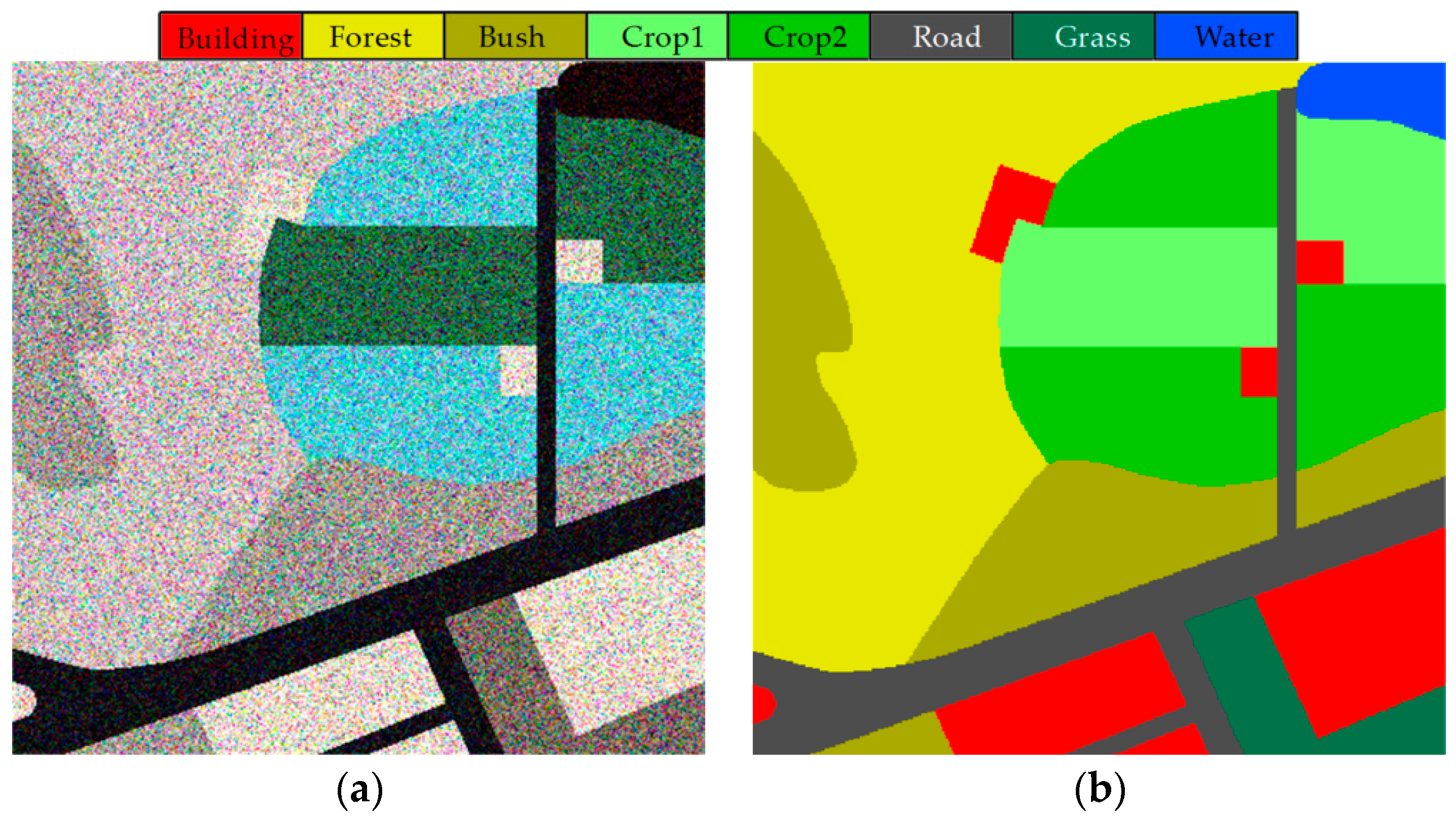
The first data set is a simulated single-look PolSAR image, 400 × 400 pixels in size, and contains eight different classes: Building areas, forest, bush land, grass land, two different types of crops, road, and a water body. To better reflect the ground reality, the Wishart distribution was adopted to generate the water body, while the G0 distribution data were adopted to generate the other classes. The initial scattering vectors and distribution parameters were estimated from a real data set. The Pauli RGB image is shown in Figure 1a, and the corresponding reference map is shown in Figure 1b. Figure 2 depicts the theoretical PDF of each class.
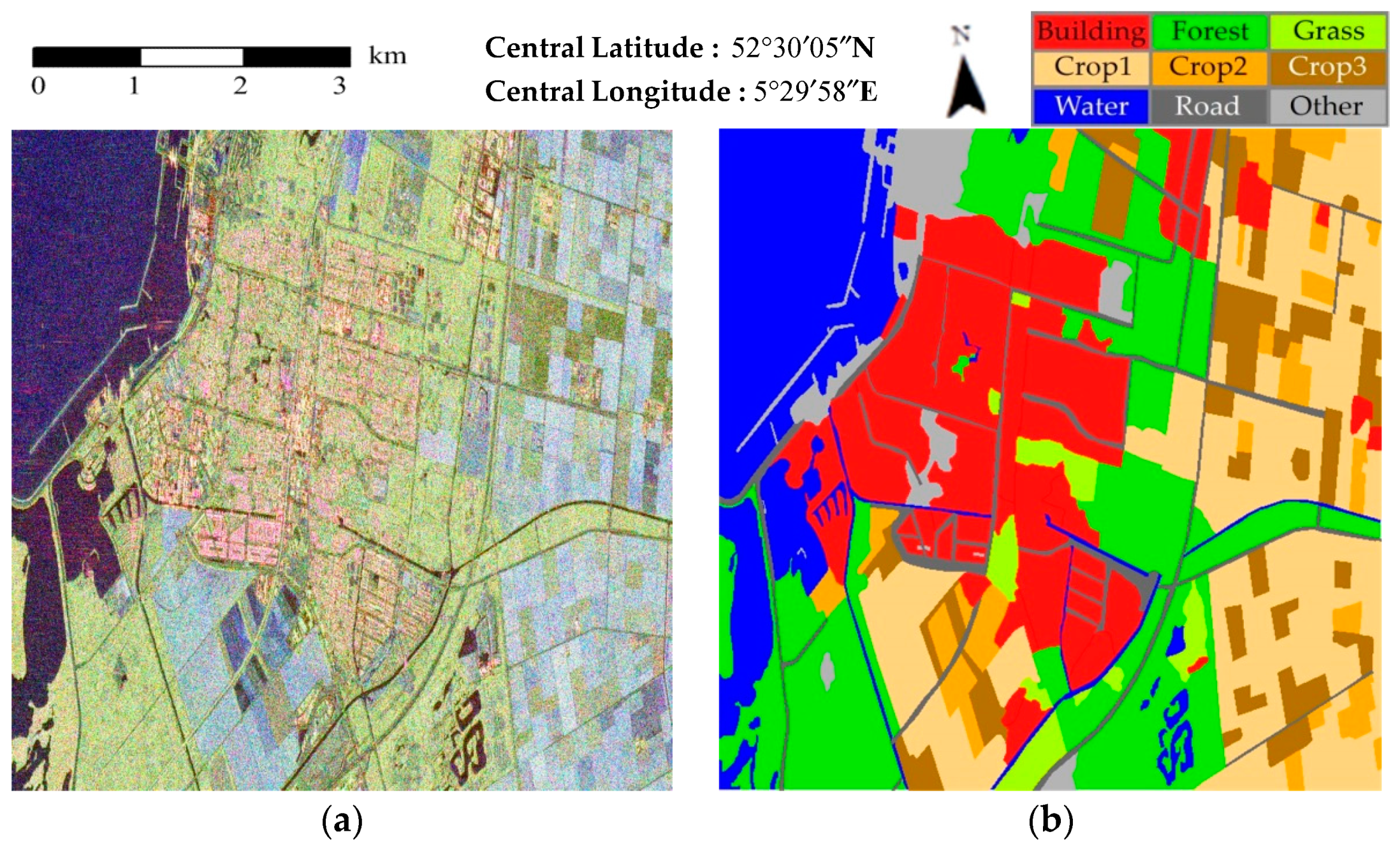
The second data set is a section of the single-look C-band RADARSAT-2 PolSAR image of Northern Flevoland, Netherlands, and has a spatial resolution of 4.7 m × 4.8 m (range × azimuth). The experimental image is 1400 × 1400 pixels in size and is shown in Figure 3a. The major land cover classes include homogeneous areas (such as water bodies and farmlands), and heterogeneous areas (such as forest and urban areas). A manual interpretation using nine categories was used as the ground truth map, which is shown in Figure 3b.
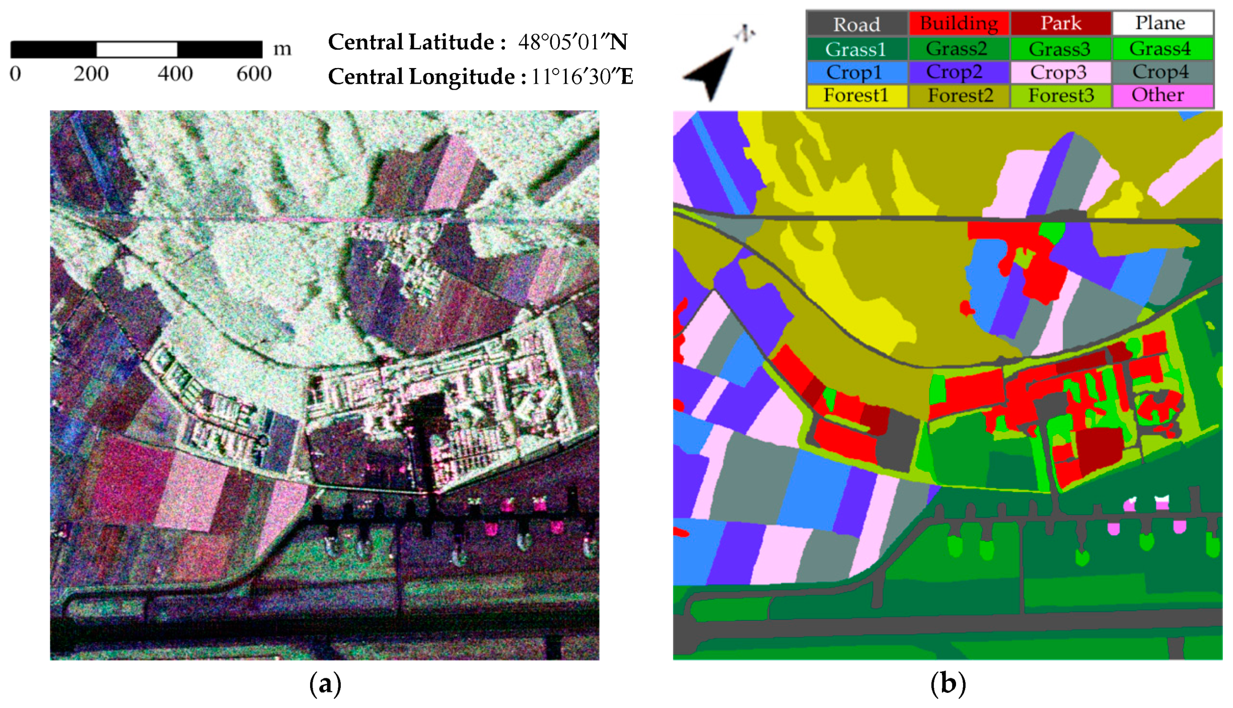
The third data set is a section of the two-look processed L-band ESAR PolSAR image of Oberpfaffenhofen, Germany, and has a spatial resolution of 1.5 m × 1.8 m (range × azimuth). The experimental image is 800 × 800 pixels in size and is shown in Figure 4a. The major land cover classes include homogeneous areas (such as roads, grasslands, and farmlands) and heterogeneous areas (such as forests and urban areas). A manual interpretation using 16 categories was used as the ground truth map, which is shown in Figure 4b.
The fourth data set is obtained from a subset of an X-band TerraSAR-X PolSAR image of Deggendorf, German, which is six-look, with a spatial resolution of about 5.0 m × 4.8 m (range × azimuth). The experimental image, with a size of 541 × 541 pixels, is shown in Figure 5a. The major land cover classes include homogeneous areas (such as river and farmlands) and heterogeneous areas (such as forests and building areas). The corresponding optical image is shown in Figure 5b.
3.2. Evaluation and Comparison
To verify the improvement in segmentation accuracy by integrating the G0 statistical features into the FNEA framework and pre-segmenting using SLIC, segmentation experiments were performed using different methods, namely: (a) FNEA segmentation based on Freeman decomposition without SAR statistical features (FFD); (b) FNEA segmentation with Pauli RGB image without SAR statistical features (FPD); (c) improved FNEA with G0 statistical features start from square blocks (IFGB); (d) improved FNEA using Wishart statistical features with pre-segmenting by SLIC (IFWS); (e) improved FNEA using K statistical features with pre-segmenting by SLIC (IFKS); (f) improved FNEA using the G0 statistical features with pre-segmenting by SLIC (IFGS); and (g) segmentation using the G0 statistical features without shape features based on SLIC pre-segmenting (IFGS-S).
In addition to qualitative visual assessment, the quality of segmentation results requires an evaluation criterion. Various accuracy metrics describe the similar aspects of the correspondence between reference objects and segments [44,45], such as the difference in area between reference objects and the segments they intersect as well as the positional difference between reference objects and segments. In this paper, area-based measures were used to evaluate the accuracy of the segmentation results. Let R denote the reference segments that consists of regions representing ground objects, and S denote segmentation result from the processed SAR image. Two area-based metrics are defined as follows:
where is the area rate of correct segmentation, i.e., detection rate, and is the degree of overlap between R and S (i.e., quality rate), which takes the false positive rate into consideration. These metrics are continuous in [0, 1], and the higher values of these metrics mean better segmentation results. Given that serious over-segmentation may also result in a high segmentation accuracy, the total number of objects (TN) was introduced as an auxiliary evaluation criterion. In general, the number of objects should be as small as possible, in the case of satisfying accuracy requirements.
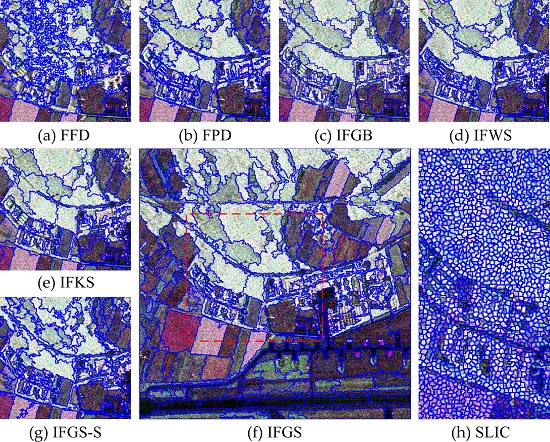
The segmentation results and accuracy measures of the simulated images using the different methods are shown in Figure 6 and Table 1, respectively. In Figure 6, the blue lines represent the boundaries of the segmentation results, and the background is the Pauli RGB image. Figure 6d shows the local details in the lower left part of the superpixel map, which was produced using SLIC with 4 × 4 pixels, in the desired size of the superpixel.
As shown in Table 1, the proposed IFGS method obtained the best detection and quality rates with the least number of generated objects, while the FFD method had the worst segmentation results. For the FFD method, inaccurate segmentation boundaries appeared, especially for classes with similar polarimetric features (Figure 6a). The results of the Pauli-based FPD method is greatly affected by speckle noise, which causes blurred segmentation boundaries between classes of crops, bush land, forest, and building areas (Figure 6b). As shown in Figure 6c–f, the class boundaries became more accurate when statistical information was utilized. However, the Wishart-based IFWS method is not applicable to heterogeneous areas like forests and urban areas. The K-based IFKS method had inaccurate segmentation results in extreme heterogeneous building areas, as shown in the bottom part of Figure 6e. In contrast, the G0-based IFGS method obtained the best segmentation results for the areas with different degrees of heterogeneity, with a 98.77% detection rate and a 97.57% quality rate. The contrast between Figure 6c,f demonstrates that dentate boundaries appear when square blocks are taken as the initial samples for the statistical model. The boundaries of straight roads or other regular areas deviated. Compared to the IFGS method, the IFGS-S method obtained the wrong segmentation boundaries in partial regular building areas, due to the absence of utilizing the shape features as shown in Figure 6g. In conclusion, the proposed superpixel-based IFGS method, utilizing the G0 distribution and shape features, obtained accurate and precise segmentation boundaries for the different areas.
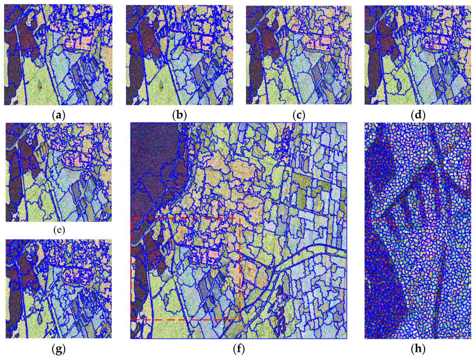
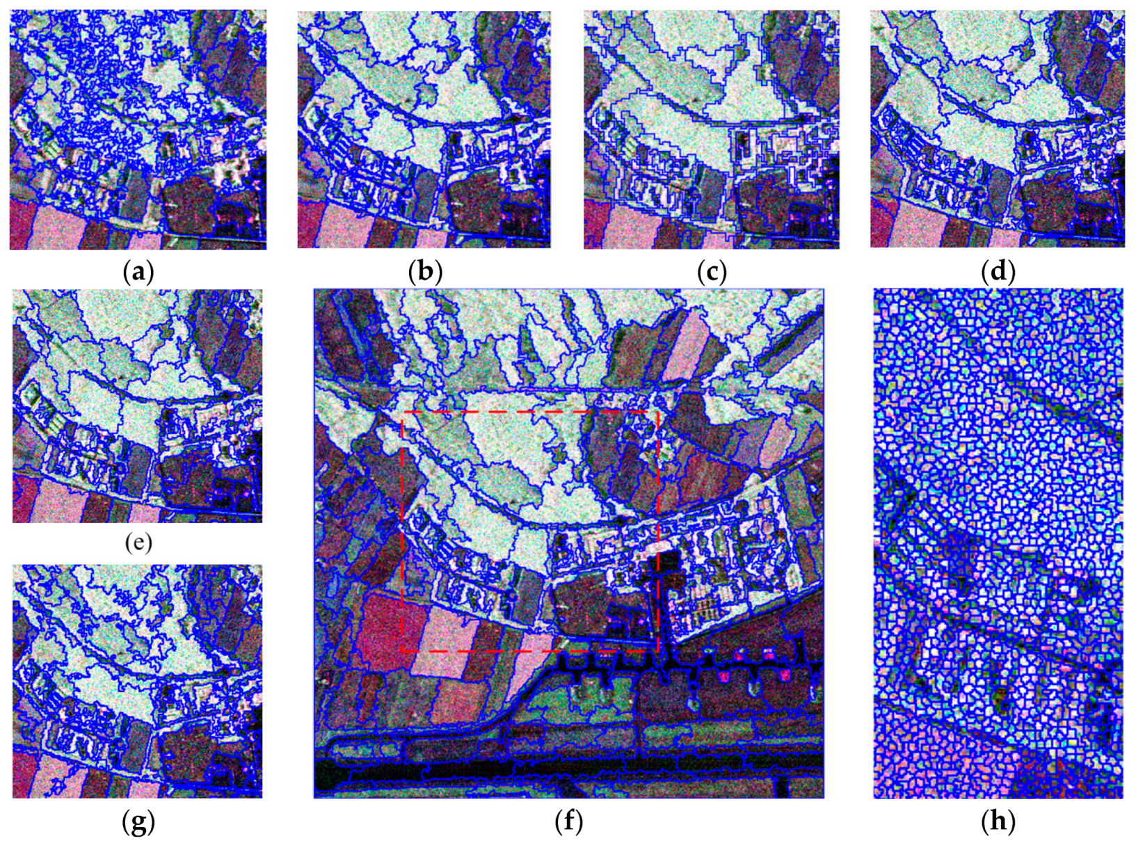
The segmentation results and superpixel map of single-look RADARSAT-2 and two-look ESAR PolSAR images, using these different methods are shown in Figure 7 and Figure 8, respectively. In Figure 7 and Figure 8, the blue lines represent the boundaries of the segmentation results, and the background is a Pauli RGB image. The superpixel maps of the RADARSAT-2 and ESAR images were produced using SLIC, with 4 × 4 pixels, in the desired size of the superpixel. The segmentation accuracies are presented in Table 2 and Table 3, respectively.
For the single-look RADARSAT-2 image, the proposed IFGS method also obtained optimal segmentation results. The contrast between Figure 7a,b and Figure 7c–f demonstrated that the utilization of statistical information helped to suppress the influence of the speckle noise, and generated accurate class boundaries. The segmentation results in Figure 7c,f certify that the superpixel-based method could avoid serrated boundaries. Moreover, the detection rate and quality rate of the IFGS method increased by approximately 1% and 1.4%, compared to the IFGB method, according to Table 2, which validated the effectiveness of the superpixels. As shown in Figure 7d–f and Table 2, the Wishart-based IFWS method obtained seriously fragmented results in areas of high heterogeneity, like the city areas located in the upper right of Figure 7d, and the K-based IFKS method had difficulty segmenting the small rivers accurately. Compared to the IFGS method, the IFGS-S method achieved blurred segmentation boundaries in urban areas, forest, and water areas due to the absence the shape feature. In summary, employing shape features and statistics information comprehensively contributed to generating better segmentation results. According to Table 2, the proposed superpixel-based IFGS method obtained the highest accuracy with the least number of segmentation objects, and the detection rate and quality rate were 91.33% and 81.53%, respectively. The above-mentioned results indicate that the proposed method is applicable to single-look high-resolution PolSAR images.
For the multi-look ESAR image, the proposed IFGS method still obtained optimal segmentation results. As shown in Figure 8a,b, the segmentation results of the FFD and FPD methods, which utilized polarimetric decomposition features, were greatly affected by the speckle noise, resulting in blurred segmentation boundaries. In contrast, the statistics-based segmentation method suppressed the influence of speckle noise and achieved more accurate segmentation boundaries between the different classes, as shown in Figure 8c–f. However, when the square blocks were taken as initial samples for the statistical models, serrated and inaccurate segmentation boundaries occurred, as shown in Figure 8c. The contrast between Figure 8d–f certifies that the G0-based IFGS method obtained better segmentation results (such as for roads in the forest) than the Wishart-based IFWS or the K-based IFKS method. For the IFGS-S method, the blurred segmentation boundaries occurred in areas with little change in statistics and polarimetric information, especially for the inner areas of forest, urban, and farmland in Figure 8g. According to Table 3, the proposed IFGS method obtained the highest accuracy with the least number of segmentation objects, similar to that of the single-look RADARSAT-2 image. Specifically, the detection and quality rates of the IFGS method were 88.46% and 72.07%, respectively. This demonstrates the effectiveness of the proposed method for multi-look high-resolution PolSAR images.
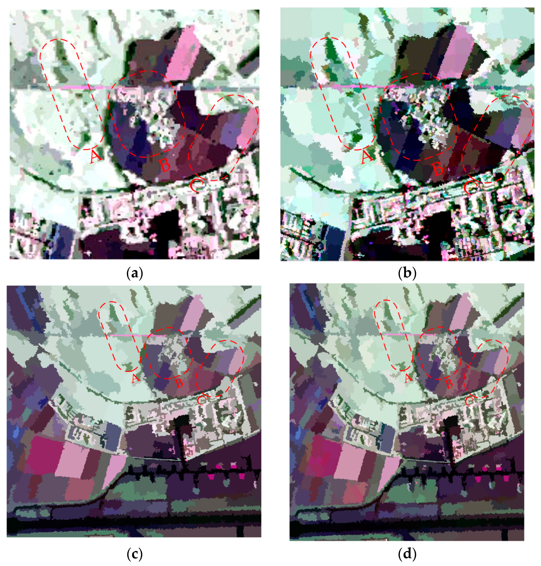
In order to further validate the effectiveness of the proposed method, the segmentation results of the third set of ESAR data, generated using the GSRM method [5] and the MW-WMRF method [15] were used as comparison. Figure 9a,b demonstrates the representation maps of the GSRM method and the MW-WMRF method, respectively. The Pauli RGB of each pixel was replaced by the average Pauli RGB of the segment that the pixel belonged to. Similarly, Figure 9c,d gives the representation maps of the proposed method at different scales. Specifically, a number of isolated small segments occurred in heterogeneous areas like forest (area A of Figure 9a) and urban areas (area B of Figure 9a) for the GSRM method, which decreased the visibility and accuracy of the representation map. As for the MW-WMRF method, the segmentation results of urban areas were broken due to the utilization of the Wishart distribution, which is shown in area B of Figure 9b. The boundaries between the different types of farmlands for these two methods were inaccurate (area C of Figure 9a,b). The boundaries for forests of different height were not accurate enough (area A of Figure 9a,b). In contrast, accurate boundaries of farmlands and forest were obtained, with different segmentation scales, for the proposed method (area A and area C of Figure 9c,d), and the urban areas were entirely segmented (area B of Figure 9c,d). Furthermore, the detection rates of the GSRM, MW-WMRF, and IFGS (t = 13) method were 87.86%, 90.20%, and 90.60%, respectively. In summary, the proposed method obtained better segmentation results compared to the GSRM method and the MW-WMRF method.
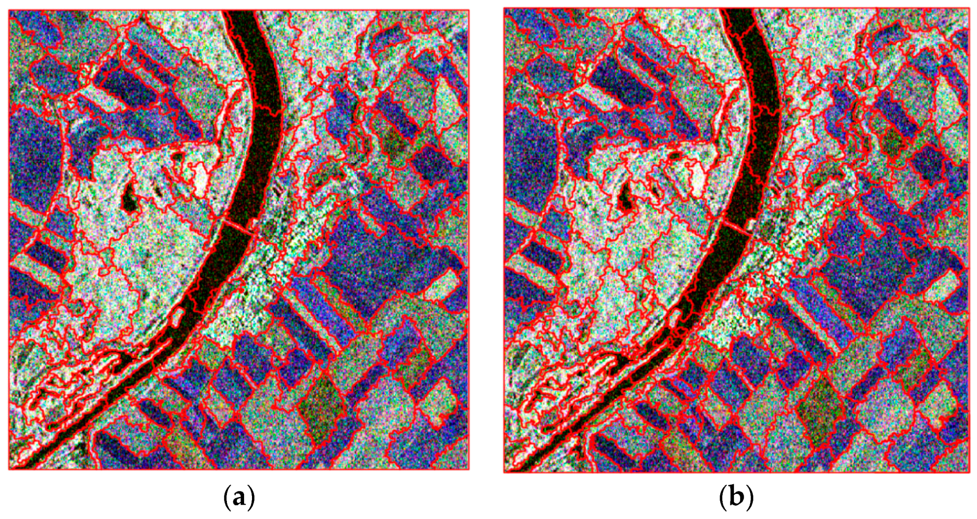
For the X-band multi-look TerraSAR-X image, the proposed IFGS method also performed well. As shown in Figure 10, the river, bridge, lakes, and building areas in the southeastern area of the river were all accurately segmented. Accurate and delicate boundaries of different types of farmlands and of the inner area of the forest were achieved. Compared to Figure 10a, the segmentation results in Figure 10b were more precise and obtained a higher quantity of objects when the segmentation scale decreased to 12. This experiment further demonstrated the applicability of the proposed method for high-resolution PolSAR images.
4. Discussion
4.1. Main Features of the Proposed Method
A superpixel-based FNEA segmentation method for high-resolution PolSAR data, using Pauli polarimetric, spatial, and G0 distribution statistical features, is proposed. The proposed method was successfully applied to simulated and real-world PolSAR data sets.
The main feature of the method is the comprehensive utilization of G0 distribution and shape information, based on FNEA. In related studies, traditional FNEA used polarimetric and geometric shape features for PolSAR image segmentation [8,9,25,26], which is easily influenced by speckle noise. Given the absence of statistical characteristics for PolSAR data, the statistical feature is introduced into the FNEA framework in the proposed approach. Many other methods use the classical complex Wishart distribution in order to represent scattering matrix statistics for PolSAR image segmentation [15,17,19,20,21,27]. Considering the ability to modeling varying degrees of texture [30,36], G0 distribution is more suitable for heterogeneous or homogeneous areas in high-resolution PolSAR data compared to the Wishart or K distribution. Thus, the proposed method adopts the G0 distribution to suppress speckle noise and obtains consistent segmentation results compared with the traditional FNEA method.
Another feature of our method is adding pre-segmentation using SLIC with the polarimetric features in order to generate initial samples for the application of the G0 statistical model. It is essential to robustly estimate model parameters with enough samples. Most of the previous work collected initial samples from image blocks within square windows [32], which led to segmentation results with obvious dentate boundaries. To handle this problem, superpixels were introduced for pre-segmentation in the proposed approach. Given the excellent boundary adherence, SLIC was used in our approach, which combined the polarimetric distance of Pauli RGB compositions and spatial distance. This approach is capable of achieving accurate segmentation results with precise boundaries between the different areas.
4.2. Sensitivity Analysis of the Parameters
According to the experiments using simulated PolSAR data and real-world PolSAR images (include RADARSAT-2 and ESAR data), the desired number of initial samples (), shape weight , and scale parameter t affected the segmentation accuracy; a detailed analysis is as follows.
4.2.1. Number of Initial Samples
As we know, an appropriate number of samples is essential for parameter estimation, namely, the size of superpixels, , affects the use of the G0 distribution in our method. When the size of the superpixels was too small, parameter estimation of the G0 distribution became unstable, which made the calculation of statistical heterogeneity inaccurate. On the other hand, statistical features were not adapted for superpixel generation. The time utilizing this statistic’s feature for the superpixel-based FNEA can be delayed when the size of superpixels become too big, which could affect the subsequent segmentation accuracy. Therefore, the proper size of a superpixel is one of key issues for the segmentation experiment.
An additional experiment was conducted to explore the minimum size of the superpixels. Abstractly, enough samples ensure stable parameter estimation of the G0 distribution, and there was little in terms of statistical heterogeneity differences between adjacent objects in one class. Three different simulated PolSAR images were used in the experiment, which only contained forest, crops, and roads, and is mentioned here in Section 3.1. The three simulated PolSAR images were divided into different sizes of blocks to calculate the standard deviation of the normalized G0 heterogeneity () between adjacent objects [32]. Figure 11 shows the changes of with different sizes of blocks. As observed in Figure 11, the standard deviation became stable when the size of the blocks was large enough. In contrast, the standard deviation increased sharply when the size of the blocks was less than 16 pixels, which means that there were large statistical heterogeneity differences, due to the unstable parameter estimation using a small number of samples. Consequently, the superpixels should contain at least 16 pixels in order to ensure the stable calculation for G0 heterogeneity.
Another experiment was conducted to analyze the effect of size of superpixels on the segmentation accuracy. In the process of generating superpixels, different desired sizes of superpixels were set, and the proposed IFGS method was used in the segmentation experiment. The changes in the detection and quality rates using the different desired sizes of superpixels for the simulated data, ESAR, and RADARSAT-2 images are shown in Figure 12. In practice, all the superpixels of a small size were merged with neighboring, larger superpixels in the generation process. The initial sizes of the superpixels were generally larger than the desired size of the superpixels. The desired sizes of the superpixels were set from 3 pixels × 3 pixels to 10 pixels × 10 pixels in this experiment.
As shown in Figure 12, the segmentation accuracy fluctuated and decreased slowly when the desired size of the superpixels increased. For the simulated image, the detection rate and quality rate decreased when the desired size of the superpixels increased from 4 pixels × 4 pixels to 10 pixels × 10 pixels. Specifically, the larger superpixels lead to delayed utilization of statistical information, and then caused a decrease in the segmentation accuracy. On the other hand, when the desired size of the superpixels was 3 pixels × 3 pixels, the number of samples could not ensure stable parameter estimation and generated inaccurate segmentation results. For the ESAR and RADARSAT-2 images, the detection rate and quality rate fluctuated when the desired size of superpixels increased due to the complexity of the real ground objects. Similarly, when the desired size of superpixels was 4 pixels × 4 pixels, the segmentation of the ESAR and RADARSAT-2 image obtained the highest detection and quality rates. Thus, superpixels were generated with a desired size of 4 pixels × 4 pixels for these three images. Sixteen pixels were used for parameter estimation of the G0 distribution for the proposed method.
4.2.2. Weight of Features
According to the previously presented segmentation experiments, shape features improved the segmentation performance for the three different images. Shape weight affected the use of statistical and shape features, according to Equation (22). In order to set an appropriate feature weight, the ratios of the average changes in shape heterogeneity and statistical heterogeneity () were calculated for the simulated data, ESAR data and RADARSAT-2 date, when the shape feature weight was 0 and 1, respectively. The ratios shown in Table 4 indicate that the shape heterogeneity was apparently larger than the statistical heterogeneity in the proposed IFGS segmentation. A relatively small shape weight should be set to balance the shape features and statistical features.
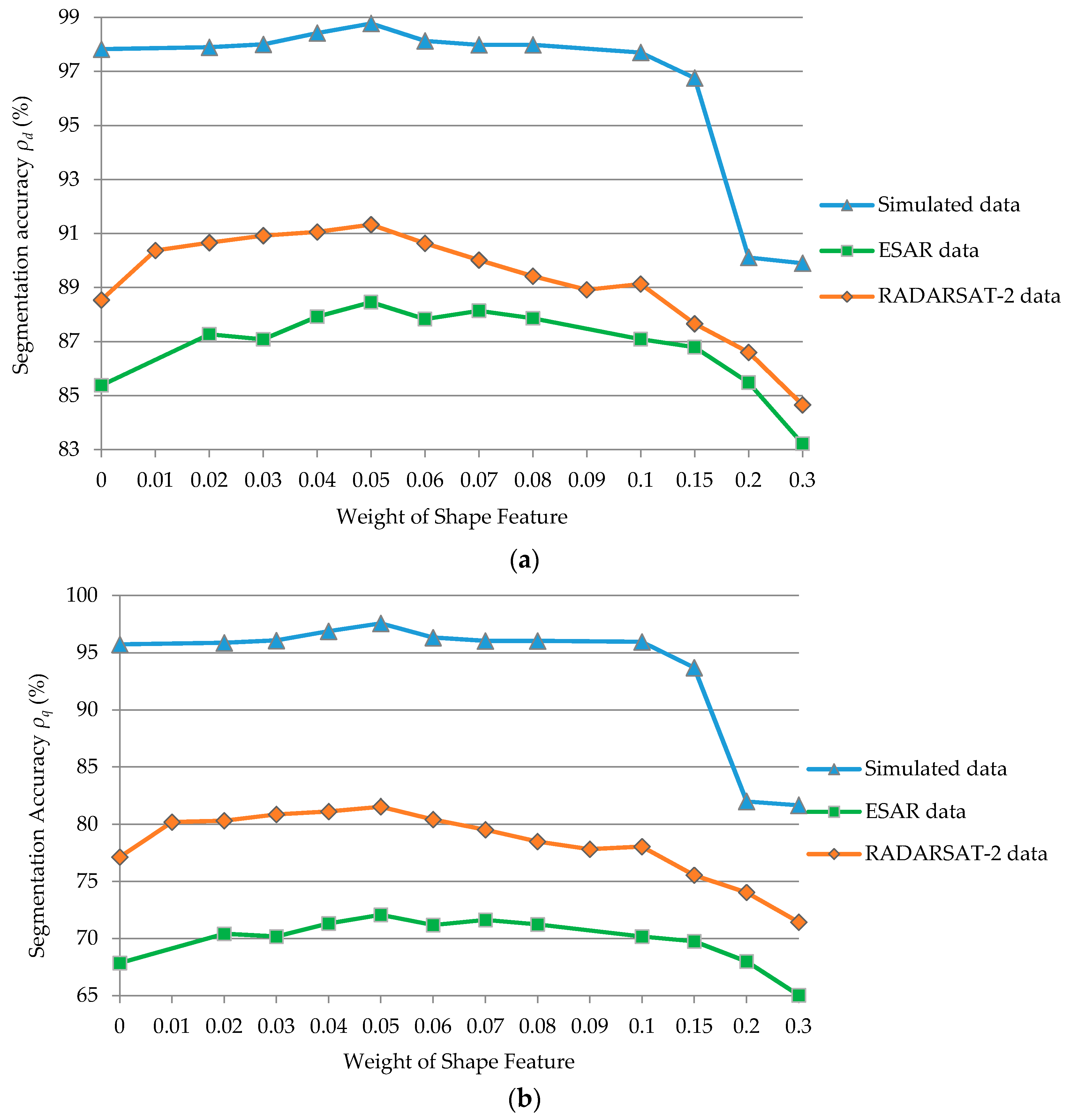
Further experiments were conducted to analyze the effects of weight of shape features on segmentation accuracy. In the process of the proposed IFGS segmentation using the desired superpixel size of 4 pixels × 4 pixels, different shape weights, in the 0–0.3 range, were set. The changes in detection and quality rates, using different shape weights for the simulated data, ESAR, and RADARSAT-2 images, are shown in Figure 13.
As shown in Figure 13, the weight of the shape also had a significant effect on the proposed IFGS segmentation method. For the simulated image, the detection rate and quality rate improved when weight of shape features increased from 0 to 0.05, and decreased when the weight of the shape features exceeded 0.05. Specifically, as the shape weight increased to more than 0.15, the relatively small statistical heterogeneity was not fully utilized, and the segmentation accuracy sharply decreased. When the shape weight varied from 0.02 to 0.08, the integrated utilization of the statistical features and shape features obtained a higher accuracy than single use of the statistical features. For the ESAR image, when the shape weight exceeded 0.1, the segmentation accuracy of the IFGS method was lower than that of the IFGS-S method. However, the same situation occurred for the RADARSAT-2 image when the shape weight exceeded 0.2, which coincided with the case where the ratios () of RADARSAT-2 image were larger than those of the ESAR image. Similar to the simulated data, when the weight of shape feature was 0.05, the segmentation of ESAR and RADARSAT-2 images obtained the highest detection and quality rates. Shape features with a weight of 0.05 were used for comprehensive utilization of shape and statistical features in the image segmentation experiment. Moreover, the detection rate of the proposed IFGS method improved by approximately 1%, 3%, and 3% compared to the IFGS-S method and the quality rate improved by approximately 2%, 4%, and 4%, respectively.
4.2.3. Scale of Segmentation
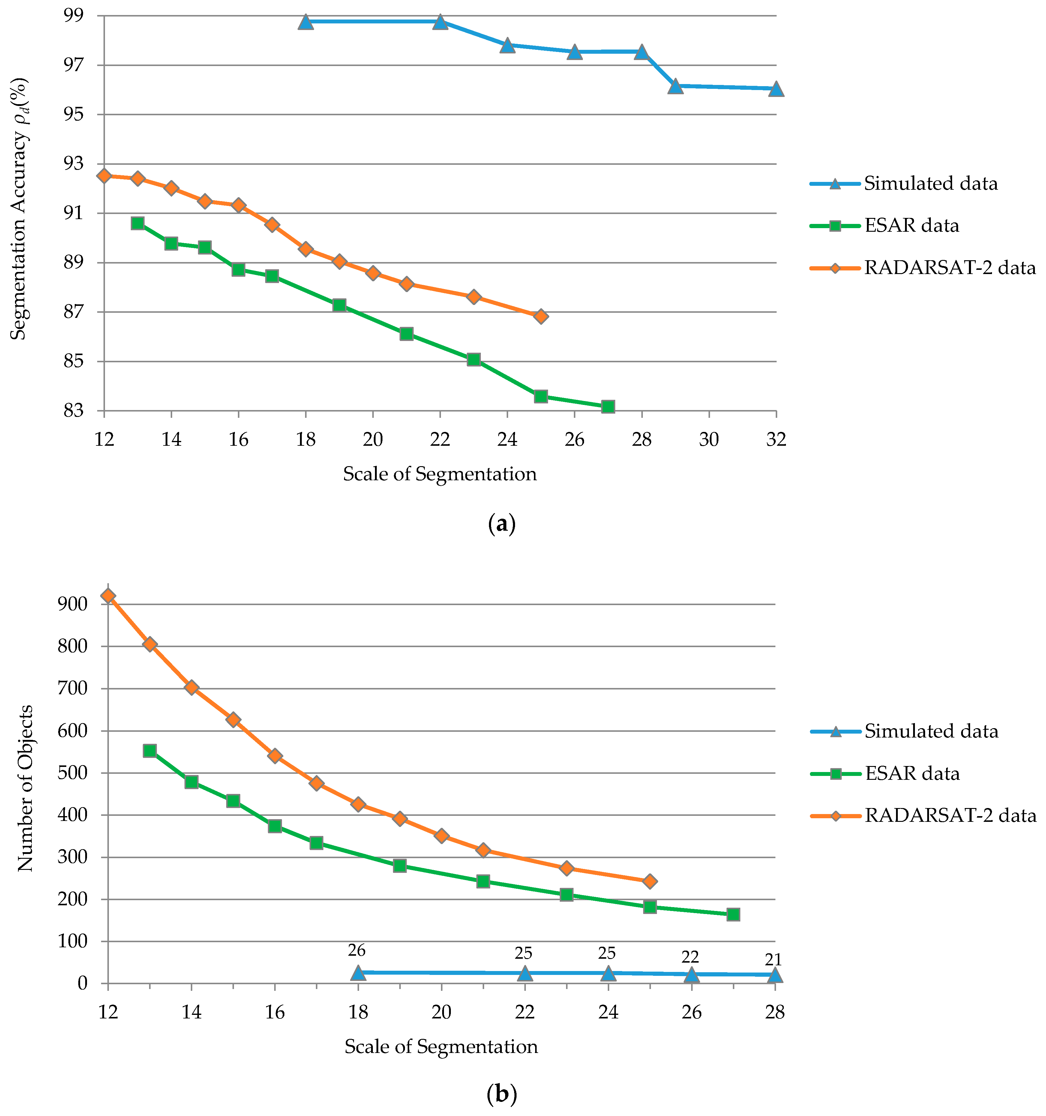
Among the three main parameters of the proposed method, scale parameter t is a relative threshold that determines the average size of objects, or the number of objects within a scene. It can be flexibly adjusted, depending on the desired number of objects in the segmentation. An extra experiment was conducted to analyze the effects of scale parameter on segmentation accuracy. In this segmentation experiment, the desired superpixel size was set as 4 pixels × 4 pixels, and the shape weight was 0.05. Different scales were set, and the detection rate and the number of result objects were calculated. Figure 14 shows the changes in the detection rate and the number of result objects with different segmentation scales for the simulated data, ESAR, and RADARSAT-2 images.
As shown in Figure 14, the scale had a consistent effect on the proposed IFGS segmentation method for the three images. As the scale of the segmentation increased, more adjacent objects were merged and the number of final objects became smaller. This means that adjacent objects with a minimal feature difference were not reasonably divided, and resulted in a decrease in segmentation accuracy. On the other hand, the number of objects and segmentation accuracy increased when the scale became smaller. However, the increased number of objects resulted in broken segmentation results. The appropriate number of objects should consider as the true application scene.
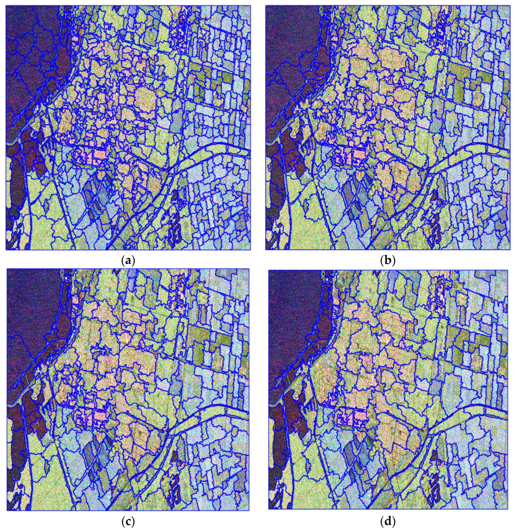
For the single-look RADARSAT-2 image, the final segmentation results using four different scales (scale = 12, 16, 20, 25) are shown in Figure 15. As the segmentation scale increased, the detail boundary information decreased and the size of single object became larger. Moreover, targets with larger areas were more intact when they were segmented. As shown in Figure 15a, the narrow rivers and roads were segmented correctly, while the heterogeneous urban areas and larger water bodies were over-segmented, causing broken segmentation results. In Figure 15d, the large water bodies were entirely segmented, but the urban areas, forest areas, and farmland were under-segmented. The boundaries of narrow roads, rivers, and small lakes were inaccurate. Incorrect boundaries occurred between adjacent objects with minimal feature differences, especially for different types of farmlands and forests. In summary, it is necessary to consider the practical use of scale-setting. Specifically, a larger scale is essential for main category classification, and larger target detection. A small scale is applicable to focusing on the details of ground objects.
4.3. Time Performance Analysis
The analysis of the proposed method consists two parts: Initial segmentation (SLIC) and superpixel-based FNEA segmentation (SP-FNEA). The time complexity of SLIC and SP-FNEA are and , respectively, where n is the number of pixels and k is the number of iterations in SP-FNEA. The time complexity of the proposed method is .
To further analyze the time efficiency of the algorithm, the runtime of SLIC and SP-FNEA for the different PolSAR images with specific segmentation scales was calculated by averaging multiple runtimes. A laptop using the 64-bit Windows 10 operating system, a quad-core Intel i5-4210U, 2.40 GHz, and 8 GB memory was utilized for the segmentation experiments. Table 5 shows the runtimes of the proposed algorithm for different PolSAR images. As shown in Table 5, the proposed algorithm has a good time efficiency. Specifically, the runtime of SLIC is linear with data size, meaning that SLIC has an excellent computational efficiency. For the SP-FNEA algorithm, its runtime efficiency is associated with the number of iterations and the data size. Generally, the larger scale resulted in the merger of adjacent objects, and increased the runtime. Moreover, the efficient SLIC avoids SP-FNEA segmentation, starting from a single pixel, and saving considerable runtime.
4.4. Accuracies, Errors, and Uncertainties
We adopted the detection and quality rates to evaluate the performance of the proposed segmentation, which were calculated according to the ground truth data. These two measures are widely considered in the field of image segmentation of remote sensing. It is clear that our method obtained more accurate segmentation results than the other methods, and this advantage was obtained with the least number of result objects.
According to the previous experiments, several factors affect the segmentation accuracy of the proposed method. The parameter estimation accuracy of the G0 distribution plays an important role in the statistical feature-based segmentation method. For the proposed approach, measurement of statistical heterogeneity and correct object merging depend on the proper estimation of the involved parameters. The determination of the scale parameters is another factor that causes segmentation errors for the proposed method. The scales of different types of targets exhibit differences due to their inequitable heterogeneities. An inappropriate scale parameter leads to under-segmentation in homogeneous regions or over-segmentation in heterogeneous regions, reducing the segmentation accuracy of the target of interest. Future development of this approach should include an accurate parameter estimation method of the G0 distribution and the determination of the segmentation scale.
The improvement of the proposed method was verified using simulated data, and real-world RADARSAT-2, ESAR, TerraSAR-X images, which mainly cover farmlands, forests, and urban areas. The experimental results show that the proposed method performed well for targets in these images. However, the segmentation results may vary for other application scenarios. In-depth experiments and analyses for other application scenarios, such as forest species classification, building collapse assessment, and oil spill extraction, have not been conducted in the present study. The applicability of the proposed method for specific applications of high-resolution PolSAR image remains uncertain.
5. Conclusions
In high-resolution fully polarimetric Synthetic Aperture Radar (PolSAR) images, speckle noise and heterogeneous regions with rich spatial features makes segmentation a challenging task. In this study, a novel segmentation algorithm for high-resolution PolSAR data has been developed by combining spatial, statistical, and polarimetric features. This integrates the statistical features into a fractal net evolution algorithm (FNEA) framework, and polarimetric features into simple linear iterative clustering (SLIC) for generating pre-segments. The main improvements are as follows: First, spectral heterogeneity in the traditional FNEA was substituted by the G0 distribution statistical heterogeneity to combine shape features and statistical features of PolSAR data. Second, a modified SLIC algorithm was utilized to generate compact, approximately homogeneous superpixels as the initial samples for the G0 statistical model, which substituted the polarimetric distance of Pauli RGB composition for the CIELAB color distance.
Several datasets were utilized in the experiments to verify the validity and applicability of the proposed method, including a simulated PolSAR data, a spaceborne single-look RADARSAT-2 image, an airborne multi-look ESAR image, and a spaceborne multi-look TerraSAR-X image. The highest accuracy for each data set was obtained using the proposed approach with the least number of generated objects, i.e., 98.77% on simulated data, 88.46% on ESAR image, and 91.33% on RADARSAT-2 image, respectively. It can thus be concluded that the proposed method achieved accurate and precise segmentation results for high-resolution PolSAR images.
Nevertheless, the performance of the proposed method could be further improved. For instance, the parameter estimation of the statistical model, the initial sample generation, the setting of the weight of features, and the strategy of determining the segmentation scale can be optimized. Moreover, the information included in the polarimetric decomposition parameters was not fully utilized in our method, except in the SLIC pre-segmentation. Hence, combining polarimetric features adequately in the superpixel-based FNEA to improve the performance of high-resolution PolSAR image segmentation is a promising prospect.
Acknowledgments
This work is supported in part by the National Natural Science Foundation of China under Grant No.41301477 and 41471355. We also thank Qi Chen and Qikai Shen for their support during the entire course of this study.
Author Contributions
Qihao Chen drafted the manuscript and was responsible for the research design, experiment; Linlin Li, Qiao Xu, Shuai Yang and Xuguo Shi reviewed the manuscript and were responsible for the analysis; Xiuguo Liu supervised the research and contributed to the editing and review of the manuscript.
Conflicts of Interest
The authors declare no conflict of interest.
References
- Jiao, L.; Liu, F. Wishart deep stacking network for fast POLSAR image classification. IEEE Trans. Image Process. 2016, 25, 3273–3286. [Google Scholar] [CrossRef] [PubMed]
- Yang, S.; Chen, Q.; Yuan, X.; Liu, X. Adaptive coherency matrix estimation for polarimetric SAR imagery based on local heterogeneity coefficients. IEEE Trans. Geosci. Remote Sens. 2016, 54, 6732–6745. [Google Scholar] [CrossRef]
- Ressel, R.; Singha, S. Comparing near coincident space borne C and X band fully polarimetric SAR data for arctic sea ice classification. Remote Sens. 2016, 8, 198. [Google Scholar] [CrossRef]
- Wei, J.; Zhang, J.; Huang, G.; Zhao, Z. On the use of cross-correlation between volume scattering and helix scattering from polarimetric SAR data for the improvement of ship detection. Remote Sens. 2016, 8, 74. [Google Scholar] [CrossRef]
- Lang, F.; Yang, J.; Li, D.; Zhao, L.; Shi, L. Polarimetric SAR image segmentation using statistical region merging. IEEE Geosci. Remote Sens. Lett. 2014, 11, 509–513. [Google Scholar] [CrossRef]
- Liu, H.; Wang, Y.; Yang, S.; Wang, S.; Feng, J.; Jiao, L. Large polarimetric SAR data semi-supervised classification with spatial-anchor graph. IEEE J. Sel. Top. Appl. Earth Obs. Remote Sens. 2016, 9, 1439–1458. [Google Scholar] [CrossRef]
- Cheng, J.; Ji, Y.; Liu, H. Segmentation-based PolSAR image classification using visual features: RHLBP and color features. Remote Sens. 2015, 7, 6079–6106. [Google Scholar] [CrossRef]
- Qi, Z.; Yeh, A.G.; Li, X.; Lin, Z. A novel algorithm for land use and land cover classification using RADARSAT-2 polarimetric SAR data. Remote Sens Environ. 2012, 118, 21–39. [Google Scholar] [CrossRef]
- Qi, Z.; Yeh, A.G.; Li, X.; Xian, S.; Zhang, X. Monthly short-term detection of land development using RADARSAT-2 polarimetric SAR imagery. Remote Sens Environ. 2015, 164, 179–196. [Google Scholar] [CrossRef]
- Suresh, G.; Melsheimer, C.; Koerber, J.; Bohrmann, G. Automatic estimation of oil seep locations in synthetic aperture radar images. IEEE Trans. Geosci. Remote Sens. 2015, 53, 4218–4230. [Google Scholar] [CrossRef]
- Vasile, G.; Ovarlez, J.; Pascal, F.; Tison, C. Coherency matrix estimation of heterogeneous clutter in high-resolution polarimetric SAR images. IEEE Trans. Geosci. Remote Sens. 2010, 48, 1809–1826. [Google Scholar] [CrossRef]
- Goodman, N.R. Statistical analysis based on a certain multivariate complex Gaussian distribution (an introduction). Ann. Math. Stat. 1963, 34, 152–177. [Google Scholar] [CrossRef]
- Tison, C.; Nicolas, J.M.; Tupin, F.; Maitre, H. A new statistical model for Markovian classification of urban areas in high-resolution SAR images. IEEE Trans. Geosci. Remote Sens. 2004, 42, 2046–2057. [Google Scholar] [CrossRef]
- Rignot, E.; Chellappa, R. Segmentation of polarimetric synthetic aperture radar data. IEEE Trans. Image Process. 1992, 1, 281–300. [Google Scholar] [CrossRef] [PubMed]
- Liu, B.; Zhang, Z.; Liu, X.; Yu, W. Representation and spatially adaptive segmentation for PolSAR images based on wedgelet analysis. IEEE Trans. Geosci. Remote Sens. 2015, 53, 1–13. [Google Scholar] [CrossRef]
- Beaulieu, J.M.; Touzi, R. Segmentation of textured polarimetric SAR scenes by likelihood approximation. IEEE Trans. Geosci. Remote Sens. 2004, 42, 2063–2072. [Google Scholar] [CrossRef]
- Alonso-Gonzalez, A.; Lopez-Martinez, C.; Salembier, P. Filtering and segmentation of polarimetric SAR data based on binary partition Trees. IEEE Trans. Geosci. Remote Sens. 2012, 50, 593–605. [Google Scholar] [CrossRef]
- Liu, B.; Hu, H.; Wang, H.; Wang, K.; Liu, X.; Yu, W. Superpixel-based classification with an adaptive number of classes for polarimetric SAR images. IEEE Trans. Geosci. Remote Sens. 2013, 51, 907–924. [Google Scholar] [CrossRef]
- Qin, F.; Guo, J.; Lang, F. Superpixel segmentation for polarimetric SAR imagery using local iterative clustering. IEEE Geosci. Remote Sens. Lett. 2015, 12, 13–17. [Google Scholar]
- Zhang, Y.; Zou, H.; Luo, T.; Qin, X.; Zhou, S.; Ji, K. A fast superpixel segmentation algorithm for PolSAR images based on edge refinement and revised Wishart distance. Sensors 2016, 16, 1687. [Google Scholar] [CrossRef] [PubMed]
- Ersahin, K.; Cumming, I.G.; Ward, R.K. Segmentation and classification of polarimetric SAR data using spectral graph partitioning. IEEE Trans. Geosci. Remote Sens. 2010, 48, 164–174. [Google Scholar] [CrossRef]
- Benz, U.C.; Hofmann, P.; Willhauck, G.; Lingenfelder, I.; Heynen, M. Multi-resolution, object-oriented fuzzy analysis of remote sensing data for GIS-ready information. ISPRS J. Photogramm. Remote Sens. 2004, 58, 239–258. [Google Scholar] [CrossRef]
- Hay, G.J.; Blaschke, T.; Marceau, D.J.; Bouchard, A. A comparison of three image-object methods for the multiscale analysis of landscape structure. ISPRS J. Photogramm. Remote Sens. 2003, 57, 327–345. [Google Scholar] [CrossRef]
- Burnett, C.; Blaschke, T. A multi-scale segmentation/object relationship modelling methodolgy for landscape analysis. Ecol. Model. 2003, 168, 233–249. [Google Scholar] [CrossRef]
- Benz, U.; Pottier, E. Object based analysis of polarimetric SAR data in alpha-entropy-anisotropy decomposition using fuzzy classification by eCognition. In Proceedings of the IEEE International Geoscience and Remote Sensing Symposium, Sydney, Australia, 9–13 July 2001; pp. 1427–1429. [Google Scholar]
- Gao, H.; Yang, K.; Jia, Y.L. Segmentation of polarimetric SAR image using object-oriented strategy. In Proceedings of the 2nd International Conference on Remote Sensing, Environment and Transportation Engineering, Nanjing, China, 1–3 June 2012; pp. 1–5. [Google Scholar]
- Cao, F.; Hong, W. An unsupervised segmentation with an adaptive number of clusters using the SPAN/H/α/A space and the complex Wishart clustering for fully polarimetric SAR data analysis. IEEE Trans. Geosci. Remote Sens. 2007, 45, 3454–3467. [Google Scholar] [CrossRef]
- Ulaby, F.T.; Kouyate, F.; Brisco, B.; Williams, T.H.L. Textural information in SAR images. IEEE Trans. Geosci. Remote Sens. 1986, GE-24, 235–245. [Google Scholar] [CrossRef]
- Quegan, S.; Rhodes, I.; Caves, R. Statistical models for polarimetric SAR data. In Proceedings of the IEEE International Geoscience and Remote Sensing Symposium, Pasadena, CA, USA, 8–12 August 1994; pp. 1371–1373. [Google Scholar]
- Freitas, C.; Frery, A.; Correia, A. The polarimetric G distribution for SAR data analysis. Environmetrics 2005, 16, 13–31. [Google Scholar] [CrossRef]
- Bombrun, L.; Beaulieu, J.M. Fisher distribution for texture modeling of polarimetric SAR data. IEEE Geosci. Remote Sens. Lett. 2008, 5, 512–516. [Google Scholar] [CrossRef]
- Bombrun, L.; Vasile, G.; Gay, M.; Totir, F. Hierarchical segmentation of polarimetric SAR images using heterogeneous clutter models. IEEE Trans. Geosci. Remote Sens. 2011, 49, 726–737. [Google Scholar] [CrossRef]
- Salembier, P.; Foucher, S. Optimum graph cuts for pruning binary partition trees of polarimetric SAR images. IEEE Trans. Geosci. Remote Sens. 2016, 54, 5493–5502. [Google Scholar] [CrossRef]
- Feng, J.; Cao, Z.; Pi, Y. Polarimetric contextual classification of PolSAR images using sparse representation and superpixels. Remote Sens. 2014, 6, 7158–7181. [Google Scholar] [CrossRef]
- Achanta, R.; Shaji, A.; Smith, K.; Lucchi, A.; Fua, P.; Süsstrunk, S. SLIC superpixels compared to state-of-the-art superpixel methods. IEEE Trans. Pattern Anal. Mach. Intell. 2012, 34, 2274–2282. [Google Scholar] [CrossRef] [PubMed]
- Khan, S.; Guida, R. Application of Mellin-kind statistics to polarimetric G distribution for SAR data. IEEE Trans. Geosci. Remote Sens. 2014, 52, 3513–3528. [Google Scholar] [CrossRef]
- Khan, S.; Guida, R. On single-look multivariate G distribution for PolSAR data. IEEE J. Sel. Top. Appl. Earth Obs. Remote Sens. 2012, 5, 1149–1163. [Google Scholar] [CrossRef]
- Gini, F.; Greco, M. Covariance matrix estimation for CFAR detection in correlated heavy tailed clutter. Signal Process. 2002, 82, 1847–1859. [Google Scholar] [CrossRef]
- Anfinsen, S.N.; Eltoft, T. Application of the matrix-variate Mellin transform to analysis of polarimetric radar images. IEEE Trans. Geosci. Remote Sens. 2011, 49, 2281–2295. [Google Scholar] [CrossRef]
- Doulgeris, A.P.; Anfinsen, S.N.; Eltoft, T. Classification with a non-Gaussian model for PolSAR data. IEEE Trans. Geosci. Remote Sens. 2008, 46, 2999–3009. [Google Scholar] [CrossRef]
- Cloude, S.R.; Pottier, E. A review of target decomposition theorems in radar polarimetry. IEEE Trans. Geosci. Remote Sens. 1996, 34, 498–518. [Google Scholar] [CrossRef]
- Jiao, H.; Luo, Y.; Wang, N.; Qi, L.; Dong, J.; Lei, H. Underwater multi-spectral photometric stereo reconstruction from a single RGBD image. In Proceedings of the Asia-Pacific Signal and Information Processing Association Annual Summit and Conference (APSIPA), Jeju, South Korea, 13–16 December 2016; pp. 1–4. [Google Scholar]
- Xu, Q.; Chen, Q.; Yang, S.; Liu, X. Superpixel-based classification using K distribution and spatial context for polarimetric SAR images. Remote Sens. 2016, 8, 619. [Google Scholar] [CrossRef]
- Möller, M.; Lymburner, L.; Volk, M. The comparison index: A tool for assessing the accuracy of image segmentation. IEEE J. Sel. Top. Appl. Earth Obs. 2007, 9, 311–321. [Google Scholar] [CrossRef]
- Clinton, N.; Holt, A.; Scarborough, J.; Yan, L.; Gong, P. Accuracy assessment measures for object-based image segmentation goodness. Photogramm. Eng. Remote Sens. 2010, 76, 289–299. [Google Scholar] [CrossRef]
Figure 1.
Simulated single-look polarimetric synthetic aperture radar (PolSAR) data as the first data set: (a) Pauli RGB image and (b) the object spatial distribution reference map of the simulated image.
Figure 1.
Simulated single-look polarimetric synthetic aperture radar (PolSAR) data as the first data set: (a) Pauli RGB image and (b) the object spatial distribution reference map of the simulated image.

Figure 2.
The theoretical probability density function (PDF) of each simulated class.
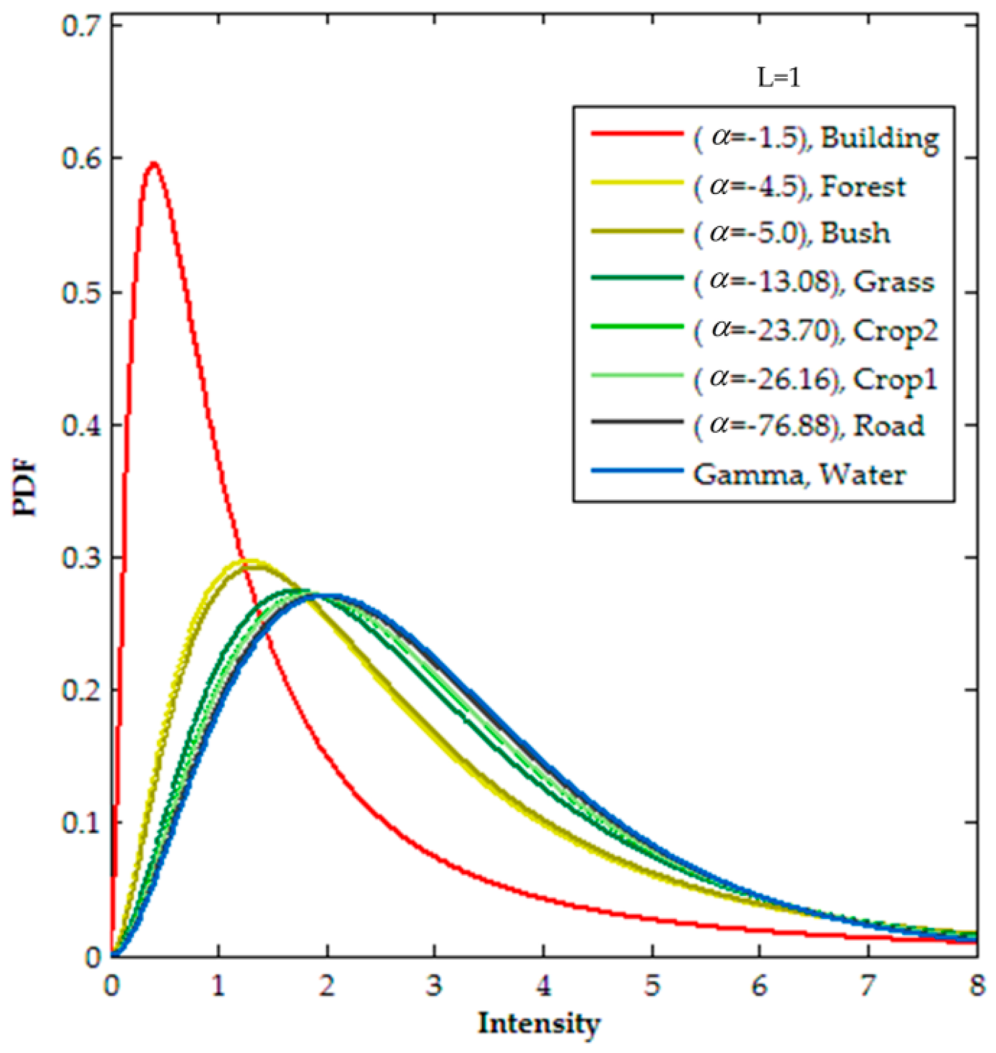
Figure 3.
C-band, single-look RADARSAT-2 PolSAR image in Flevoland as the second data set: (a) Pauli RGB image and (b) the ground truth map of (a).
Figure 3.
C-band, single-look RADARSAT-2 PolSAR image in Flevoland as the second data set: (a) Pauli RGB image and (b) the ground truth map of (a).

Figure 4.
L-band, two-look ESAR PolSAR image in Oberpfaffenhofen as the third data set: (a) Pauli RGB image and (b) the ground truth map of (a).
Figure 4.
L-band, two-look ESAR PolSAR image in Oberpfaffenhofen as the third data set: (a) Pauli RGB image and (b) the ground truth map of (a).

Figure 5.
X-band, six-look TerraSAR-X PolSAR image of Deggendorf as the fourth data set: (a) Pauli RGB image and (b) the reference image from Google Earth.
Figure 5.
X-band, six-look TerraSAR-X PolSAR image of Deggendorf as the fourth data set: (a) Pauli RGB image and (b) the reference image from Google Earth.
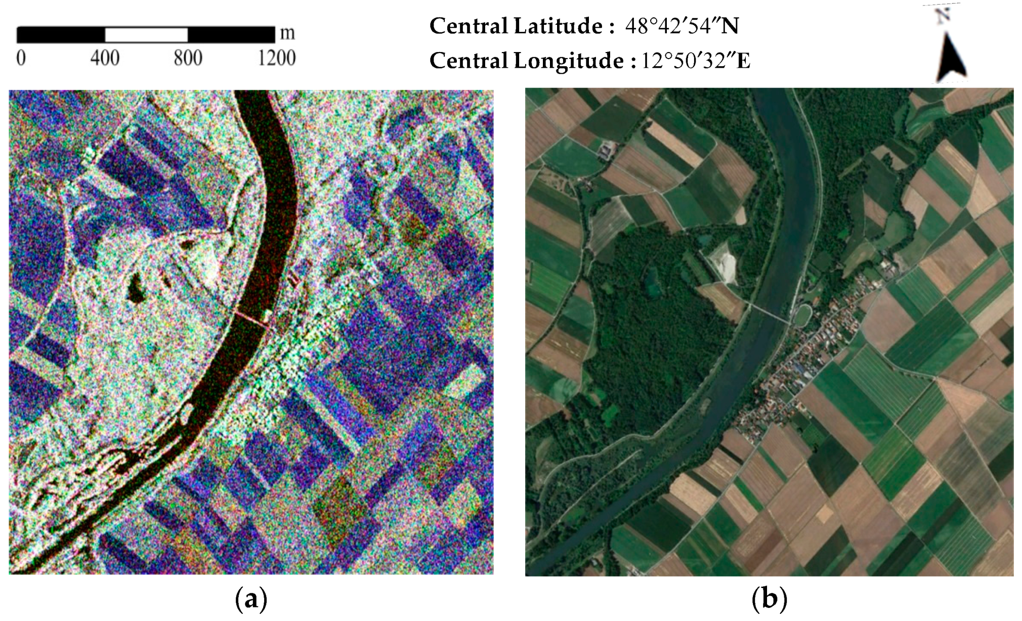
Figure 6.
Segmentation results of the simulated image using different methods: (a) FNEA segmentation based on Freeman decomposition without SAR statistical features (FFD); (b) FNEA segmentation with Pauli RGB image without SAR statistical features (FPD); (c) improved FNEA with G0 statistical features start from square blocks (IFGB); (d) improved FNEA using Wishart statistical features with pre-segmenting by simple linear iterative clustering (SLIC) (IFWS); (e) improved FNEA using K statistical features with pre-segmenting by SLIC (IFKS); (f) improved FNEA using the G0 statistical features with pre-segmenting by SLIC (IFGS); (g) segmentation using the G0 statistical features without shape features based on SLIC pre-segmenting (IFGS-S); and (h) SLIC (local enlarged drawing of lower-left part of the superpixel map).
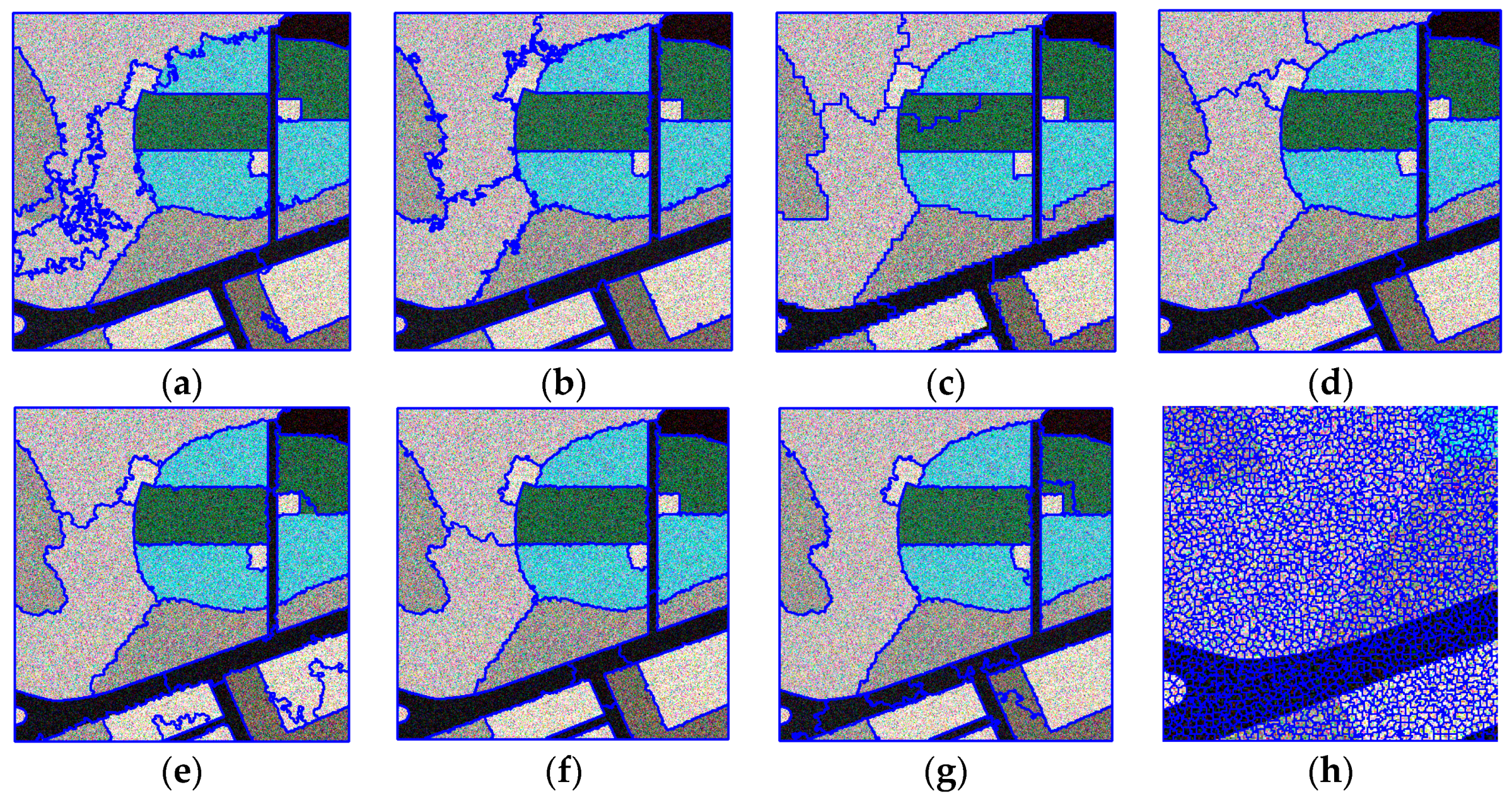
Figure 7.
Segmentation results of the single-look RADARSAT-2 PolSAR image using different methods: (a) FFD; (b) FPD; (c) IFGB; (d) IFWS; (e) IFKS; (f) IFGS; (g) IFGS-S; and (h) SLIC (local enlarged drawing of central left part of the superpixel map). (a–e,g) show screenshots of the results in the red dashed rectangle of (f).

Figure 8.
Segmentation results of the two-look ESAR PolSAR image using different methods: (a) FFD; (b) FPD; (c) IFGB; (d) IFWS; (e) IFKS; (f) IFGS; (g) IFGS-S; and (h) SLIC (local enlarged drawing of central left part of the superpixel map). (a–e,g) show screenshots of the results in the red dashed rectangle of (f).

Figure 9.
Representation maps (Pauli RGB images) of segmentation results for the ESAR data using different methods: (a) GSRM; (b) MW-WMRF; (c) IFGS, t = 17, = 0.05, = 16; and (d) IFGS, t = 13, = 0.05, = 16.
Figure 9.
Representation maps (Pauli RGB images) of segmentation results for the ESAR data using different methods: (a) GSRM; (b) MW-WMRF; (c) IFGS, t = 17, = 0.05, = 16; and (d) IFGS, t = 13, = 0.05, = 16.

Figure 10.
Segmentation results of the six-look TerraSAR-X PolSAR image using the proposed method: (a) IFGS, t = 16, = 0.05, = 16; (b) IFGS, t = 12, = 0.05, = 16.
Figure 10.
Segmentation results of the six-look TerraSAR-X PolSAR image using the proposed method: (a) IFGS, t = 16, = 0.05, = 16; (b) IFGS, t = 12, = 0.05, = 16.

Figure 11.
Standard deviation of the normalized G0 heterogeneity, as a function of block size.
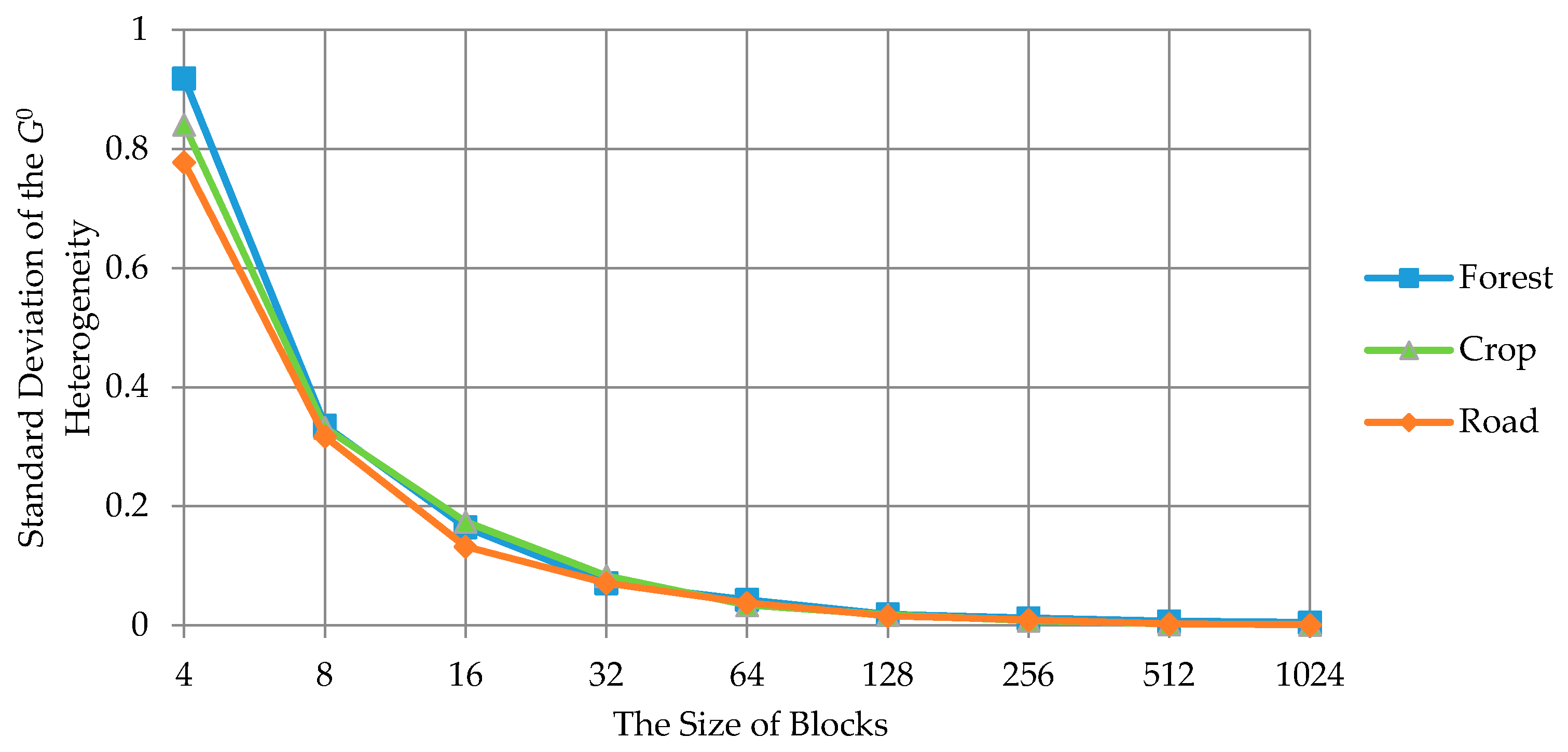
Figure 12.
Segmentation accuracy obtained using the IFGS method for the simulated data, ESAR, and RADARSAT-2 data, with different desired sizes of superpixels: (a) detection rate; (b) quality rate.
Figure 12.
Segmentation accuracy obtained using the IFGS method for the simulated data, ESAR, and RADARSAT-2 data, with different desired sizes of superpixels: (a) detection rate; (b) quality rate.
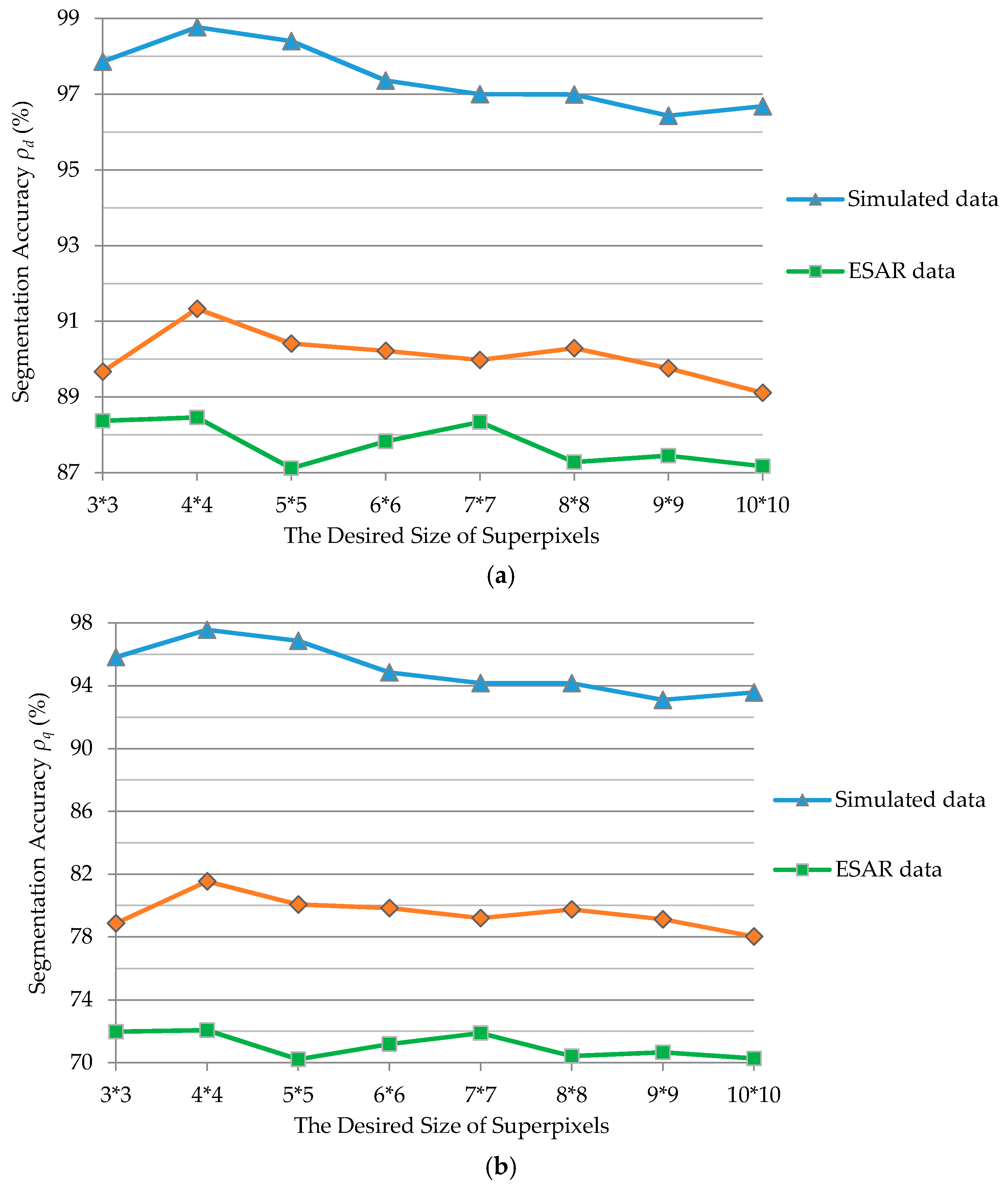
Figure 13.
Segmentation accuracy obtained using the IFGS method for the simulated data, ESAR, and RADARSAT-2 data with different shape weights: (a) detection rate; (b) quality rate.
Figure 13.
Segmentation accuracy obtained using the IFGS method for the simulated data, ESAR, and RADARSAT-2 data with different shape weights: (a) detection rate; (b) quality rate.

Figure 14.
Segmentation accuracy obtained using the IFGS method for the simulated data, ESAR, and RADARSAT-2 data with different scales: (a) detection rate; (b) the number of result objects.
Figure 14.
Segmentation accuracy obtained using the IFGS method for the simulated data, ESAR, and RADARSAT-2 data with different scales: (a) detection rate; (b) the number of result objects.

Figure 15.
Segmentation results of the single-look RADARSAT-2 PolSAR image with different scales: (a) scale = 12; (b) scale = 16; (c) scale = 20; (d) scale = 25.
Figure 15.
Segmentation results of the single-look RADARSAT-2 PolSAR image with different scales: (a) scale = 12; (b) scale = 16; (c) scale = 20; (d) scale = 25.


Table 1.
Segmentation accuracy measures of the simulated image.
| Method | (%) | (%) | TN |
|---|---|---|---|
| FFD | 94.33 | 89.27 | 26 |
| FPD | 98.22 | 96.50 | 26 |
| IFGB | 97.12 | 94.40 | 26 |
| IFWS | 98.47 | 96.98 | 26 |
| IFKS | 98.11 | 96.29 | 27 |
| IFGS | 98.77 | 97.57 | 25 |
| IFGS-S | 98.70 | 97.44 | 29 |
Table 2.
Segmentation accuracy measures of the single-look RADARSAT-2 image.
| Method | (%) | (%) | TN |
|---|---|---|---|
| FFD | 89.30 | 78.26 | 558 |
| FPD | 88.49 | 77.07 | 553 |
| IFGB | 90.35 | 80.10 | 546 |
| IFWS | 89.14 | 78.17 | 564 |
| IFKS | 89.17 | 78.03 | 543 |
| IFGS | 91.33 | 81.53 | 541 |
| IFGS-S | 89.53 | 78.68 | 590 |
Table 3.
Segmentation accuracy measures of the two-look ESAR image.
| Method | (%) | (%) | TN |
|---|---|---|---|
| FFD | 83.31 | 65.13 | 348 |
| FPD | 86.65 | 69.57 | 335 |
| IFGB | 87.90 | 71.29 | 335 |
| IFWS | 87.94 | 71.34 | 342 |
| IFKS | 87.57 | 70.82 | 334 |
| IFGS | 88.46 | 72.07 | 334 |
| IFGS-S | 85.38 | 67.85 | 343 |
Table 4.
Ratios () calculated for the simulated data, ESAR, and RADARSAT-2 image in segmentation with the shape weight of 0 and 1.
Table 4.
Ratios () calculated for the simulated data, ESAR, and RADARSAT-2 image in segmentation with the shape weight of 0 and 1.
| PolSAR Data | ||
|---|---|---|
| Simulated image | 1.48 | 2.07 |
| ESAR image | 2.09 | 2.25 |
| RADARSAT-2 image | 6.55 | 8.25 |
Table 5.
Runtimes of the proposed algorithm for different PolSAR images.
| PolSAR Data | Size | Scale t | Time (s) | ||
|---|---|---|---|---|---|
| SLIC | SP-FNEA | Total | |||
| Simulated Data | 400 × 400 | 22 | 22.52 | 12.32 | 34.84 |
| RADARSAT-2 | 1400 × 1400 | 16 | 267.85 | 238.60 | 506.45 |
| ESAR | 800 × 800 | 17 | 88.04 | 64.66 | 152.70 |
| TerraSAR-X | 541 × 541 | 16 | 40.07 | 27.20 | 67.27 |
© 2017 by the authors. Licensee MDPI, Basel, Switzerland. This article is an open access article distributed under the terms and conditions of the Creative Commons Attribution (CC BY) license (http://creativecommons.org/licenses/by/4.0/).
Share and Cite
MDPI and ACS Style
Chen, Q.; Li, L.; Xu, Q.; Yang, S.; Shi, X.; Liu, X. Multi-Feature Segmentation for High-Resolution Polarimetric SAR Data Based on Fractal Net Evolution Approach. Remote Sens. 2017, 9, 570. https://doi.org/10.3390/rs9060570
AMA Style
Chen Q, Li L, Xu Q, Yang S, Shi X, Liu X. Multi-Feature Segmentation for High-Resolution Polarimetric SAR Data Based on Fractal Net Evolution Approach. Remote Sensing. 2017; 9(6):570. https://doi.org/10.3390/rs9060570
Chicago/Turabian StyleChen, Qihao, Linlin Li, Qiao Xu, Shuai Yang, Xuguo Shi, and Xiuguo Liu. 2017. "Multi-Feature Segmentation for High-Resolution Polarimetric SAR Data Based on Fractal Net Evolution Approach" Remote Sensing 9, no. 6: 570. https://doi.org/10.3390/rs9060570
Note that from the first issue of 2016, this journal uses article numbers instead of page numbers. See further details here.