Calibration of METRIC Model to Estimate Energy Balance over a Drip-Irrigated Apple Orchard

Abstract

A field experiment was carried out to calibrate and evaluate the METRIC (Mapping EvapoTranspiration at high Resolution Internalized with Calibration) model for estimating the spatial and temporal variability of instantaneous net radiation (Rn_i), soil heat flux (G_i), sensible heat flux (H_i), and latent heat flux (LE_i) over a drip-irrigated apple (Malus domestica cv. Pink Lady) orchard located in the Pelarco valley, Maule Region, Chile (35°25′20′′LS; 71°23′57′′LW; 189 m.a.s.l.). The study was conducted in a plot of 5.5 hectares using 20 satellite images (Landsat 7 ETM+) acquired on clear sky days during three growing seasons (2012/2013, 2013/2014 and 2014/2015). Specific sub-models to estimate G_i, leaf area index (LAI) and aerodynamic roughness length for momentum transfer (Z_om) were calibrated for the apple orchard as an improvement to the standard METRIC model. The performance of the METRIC model was evaluated at the time of satellite overpass using measurements of H_i and LE_i obtained from an eddy correlation system. In addition, estimated values of Rn_i, G_i and LAI were compared with ground-truth measurements from a four-way net radiometer, soil heat flux plates and plant canopy analyzer, respectively. Validation indicated that LAI, Z_om and G_i were estimated using the calibrated functions with errors of +2%, +6% and +3% while those were computed using the standard functions with error of +59%, +83%, and +12%, respectively. In addition, METRIC using the calibrated functions estimated H_i and LE_i with error of +5% and +16%, while using the original functions estimated H_i and LE_i with error of +29% and +26%, respectively.

1. Introduction

Water scarcity has become a main limiting factor for agriculture, especially in arid and semi-arid conditions. This issue has become particularly relevant in countries like Chile where many commercial apple orchards have been transformed from traditional to intensive (1500 tree·ha⁻¹) or super-intensive (3500 tree·ha⁻¹) planting densities that require the optimization of water application and reduction of the cost of electrical energy required for pumping water into orchards. For this reason, decision-making tools for irrigation management are needed to optimize water productivity and maintain sufficient levels of crop productivity and quality. A correct quantification of apple water consumption or actual evapotranspiration (ETa) is a key factor in improving water productivity both at orchard and regional scales.

Traditionally, ETa is calculated by multiplying the reference evapotranspiration (ETr) by a crop coefficient (Kc) which depends on crop type and the crop growth stage [1,2]. This procedure is based on the Penman–Monteith (PM) equation, which computes daily ETr values over a reference surface (alfalfa or grass) using weather-based data from an automatic weather station (AWS) [3,4]. However, the Kc values taken from literature are often not adapted to varying orchard conditions such as soil type, cultivar and climate characteristics [5,6]. In addition, Kc values for complex, heterogeneous canopies such as fruit orchards depend highly on canopy architecture, plant densities, and standard agronomical practices that determine the partitioning of ETa into transpiration and soil evaporation [7]. This issue can produce substantial error in the estimation of orchard water requirements and reduce the water use efficiency, yield and fruit quality [8].

In recent decades, remote sensing energy balance (RSEB) approaches have become a valuable technology to quantify the spatio-temporal variability of water requirements for a wide range of vegetation types [9,10,11]. To map ETa from satellite imagery, RSEB algorithms use the remotely sensed surface reflectance and radiometric surface temperature (Ts) to transform satellite radiances into land surface characteristics such as emissivity, surface albedo, vegetation indices, and surface aerodynamic temperature [12,13,14]. Thereby, satellite-based data in combination with ground-based meteorological measurements are used to compute the daily ETa as a residual from the surface energy balance equation at the time of the satellite overpass [15]:

$${\mathsf{\lambda }\mathrm{ETa}}_i={\mathrm{Rn}}_i-{\mathrm{G}}_i-{\mathrm{H}}_i$$

(1)

where λ is the latent heat of vaporization (J·kg⁻¹); ETa_i is instantaneous evapotranspiration (mm·h⁻¹); LE_i is instantaneous latent heat flux (W·m⁻²); Rn_i is instantaneous net radiation (W·m⁻²); G_i is instantaneous soil heat flux (W·m⁻²); and H_i is instantaneous sensible heat flux (W·m⁻²). Subscripts “i” denote measurements at the time of the satellite overpass (approximately 11:30 h local time).

RSEB models estimate Rn_i, G_i and H_i using surface reflectance and surface temperature from satellite platforms such as MODIS, Landsat (7 ETM+ and 8 OLI) and ASTER [12,16,17,18,19]. RSEB models have been tested extensively in different parts of the world with positive results for several fully covered crops but little research exists on the application of these algorithms to estimate ETa over heterogeneous or complex canopies such as apple orchards. In this regard, studies have indicated that the METRIC (Mapping EvapoTranspiration at high Resolution with Internalized Calibration) model is able to estimate ETa with errors ranging between 5% and 20% in fully covered crops such as beans, wheat, corn, cotton and beets [6,19,20]. Several researchers have indicated that METRIC can be used to evaluate the spatial variability of ETa and Kc of vineyards and orchards with promising results [16,18,21,22,23].

METRIC is a one-source model that uses an internal self-calibration process called CIMEC (Calibration using Inverse Modeling at Extreme Conditions) [3,6,12,16], which eliminates the need for an atmospheric correction of surface temperature and albedo measurements using the radiative transfer model [16,19]. In addition, METRIC utilizes ground-based ETr data acquired in the satellite scene to inversely and internally calibrate the surface energy balance which facilitates determining the extreme conditions of heat exchange over agricultural areas (the “hot” and “cold” pixels or anchor pixels) in order to calibrate the sensible heat flux at the pixel-level [16,24,25].

The main disadvantage of the energy balance approach employed in METRIC is that the estimation of LE_i for each pixel is only as accurate as the estimates for Rn_i, G_i and H_i [6]. In addition, sensitivity analyses applied to METRIC indicate that variations on intermediate parameters such as albedo, leaf area index (LAI), G_i and momentum roughness length (Z_om) can indirectly affect the accuracy of LE_i and subsequently ETa estimation [25,26]. Therefore, the evaluation of energy balance over heterogeneous canopies such as orchards is needed to provide insight into sources of error in the estimation of orchard ETa.

In general, sparse woody canopies such as high-density apple orchards have spacings between rows that vary with canopy geometry and planting density and that affect the partitioning of Rn_i into G_i, H_i and LE_i [27]. Therefore, a satellite-pixel integrates a mixture of different surface temperatures, e.g. the shaded and illuminated portion of the canopy in combination with the shaded and sunlit surface of bare soil at the moment of satellite overpass which can lead to bias in the estimation of H_i [23] due to variation in sun angle and satellite viewing angle. To minimize these effects, a correction is required in the sub-models that compute G_i, LAI and Z_om [18]. In addition, Santos et al. (2012) [23] reported that the estimations of H_i may be biased by uncertainty in the modeling of Z_om which is a measure of resistance and friction between the air layer that interacts with the surface of crops [17]. In the case of fruit orchards, Z_om increases in proportion to the crop density until a density threshold of approximately LAI = 3 m²·m^-2 is achieved when the trees have a uniform distribution of the leaves in the canopy [3].

Therefore, the application of METRIC to estimate orchard water requirements requires specific adjustment of sub-models that estimate LAI, G_i and Z_om. Thus, the main goals of this research were to calibrate the sub-models to compute LAI, G_i and Z_om and to validate the METRIC model to compute the instantaneous values of Rn_i, G_i, H_i and LE_i over a drip-irrigated apple orchard under Mediterranean semi-arid climatic conditions.

Original METRIC Model

METRIC uses TIR-Multispectral satellite images (e.g., from Landsat 7 ETM+ and 8 OLI) and ground-based meteorological data to estimate pixel-based daily ETa at 30 × 30 m spatial resolution via a surface energy balance equation at the time of the satellite overpass (Equation (1)). Rn_i (W·m⁻²) is calculated pixel by pixel as [17]:

$${\mathrm{Rn}}_{i\_\mathrm{M}}=\left(1-\alpha \right)·{\mathrm{R}}_{\mathrm{S}\downarrow }+{\mathrm{R}}_{\mathrm{L}\downarrow }-{\mathrm{R}}_{\mathrm{L}\uparrow }-\left(1-{ℰ}_{\mathrm{o}}\right)·{\mathrm{R}}_{\mathrm{L}\downarrow }$$

(2)

where α is surface albedo (dimensionless), R_s↓ is the incoming short-wave radiation (W·m⁻²), R_L↓ is the incoming long-wave radiation (W·m⁻²), and R_L↑ is the outgoing long-wave radiation (W m⁻²). ε_o is broadband surface thermal emissivity (dimensionless). The subscript “_M” indicates values computed by METRIC.

In the METRIC algorithm [6], values for G_i are estimated as follows [28]:

$$\frac{{\mathrm{G}}_{i\_\mathrm{M}}}{{\mathrm{Rn}}_{i\_\mathrm{M}}}=\mathrm{Ts}·\left({\mathrm{c}}_1+{\mathrm{c}}_1·\alpha \right)·\left(1-0.98·{\mathrm{NDVI}}^4\right)$$

(3)

where Ts is the radiometric surface temperature (°C) estimated from the TIR band and NDVI is the normalized difference vegetation index. For homogenous canopies, values of c₁ and c₂ are 0.0038 and 0.0074, respectively.

For short annual crops, LAI (m²·m⁻²) is estimated as [17]:

$$\mathrm{LAI}=11·{\mathrm{SAVI}}^3\mathrm{SAVI}\le 0.817$$

(4)

$$\mathrm{LAI}=6\mathrm{SAVI}>0.817$$

(5)

where SAVI is the soil adjusted vegetation Index (dimensionless) calculated using the top of atmospheric reflectance.

Values for H_i (W·m⁻²) are obtained for each pixel as [16]:

$${\mathrm{H}}_{i\_\mathrm{M}}={\rho }_{\mathrm{air}}·{\mathrm{C}}_{\mathrm{P}}·\frac{\Delta \mathrm{Ts}}{{\mathrm{r}}_{\mathrm{ah}}}$$

(6)

where ρ_air is air density (kg·m⁻³); C_p is specific heat of air at constant pressure (1004 J·kg⁻¹·K⁻¹); and ΔTs is the near-surface air temperature gradient (ΔTa = Ta_z1 − Ta_z2) above each pixel, where Ta_z1 and Ta_z2 are near surface air temperature (°K) at heights z₁ and z₂ above the elevation of d + Z_om, where d is zero plane displacement height (all in m). r_ah is the aerodynamic resistance to heat transport (s·m⁻¹). Details on estimating r_ah and H_{i_M} are described by [16] and include correction for effects of buoyancy.

To estimate the ΔTs, two anchor pixels are selected in the study area corresponding to cold and hot pixels in order to apply the CIMEC process [6,16]. The cold pixel is defined and located over a well-watered and non-stressed agricultural area, which represents the maximum value of ETa, while the hot pixel is located in a bare soil agricultural area where ETa is nearly zero [29]. The internal calibration reduces impact of any biases in estimation of aerodynamic stability correction and surface roughness [16]. ΔTs is linearly calculated at all pixels as:

$$\Delta \mathrm{Ts}=a+b·\mathrm{Ts}$$

(7)

where a and b are empirically determined constants for a given satellite image and Ts is the surface temperature (°K) adjusted to a common elevation datum for each image/pixel using a digital elevation model and customized de-lapsing rate.

METRIC estimates Z_om of annual agricultural crops assuming that the crop height varies proportionally with the LAI, as [17]:

$${\mathrm{Z}}_{\mathrm{om}}=0.018·\mathrm{LAI}$$

(8)

2. Materials and Methods

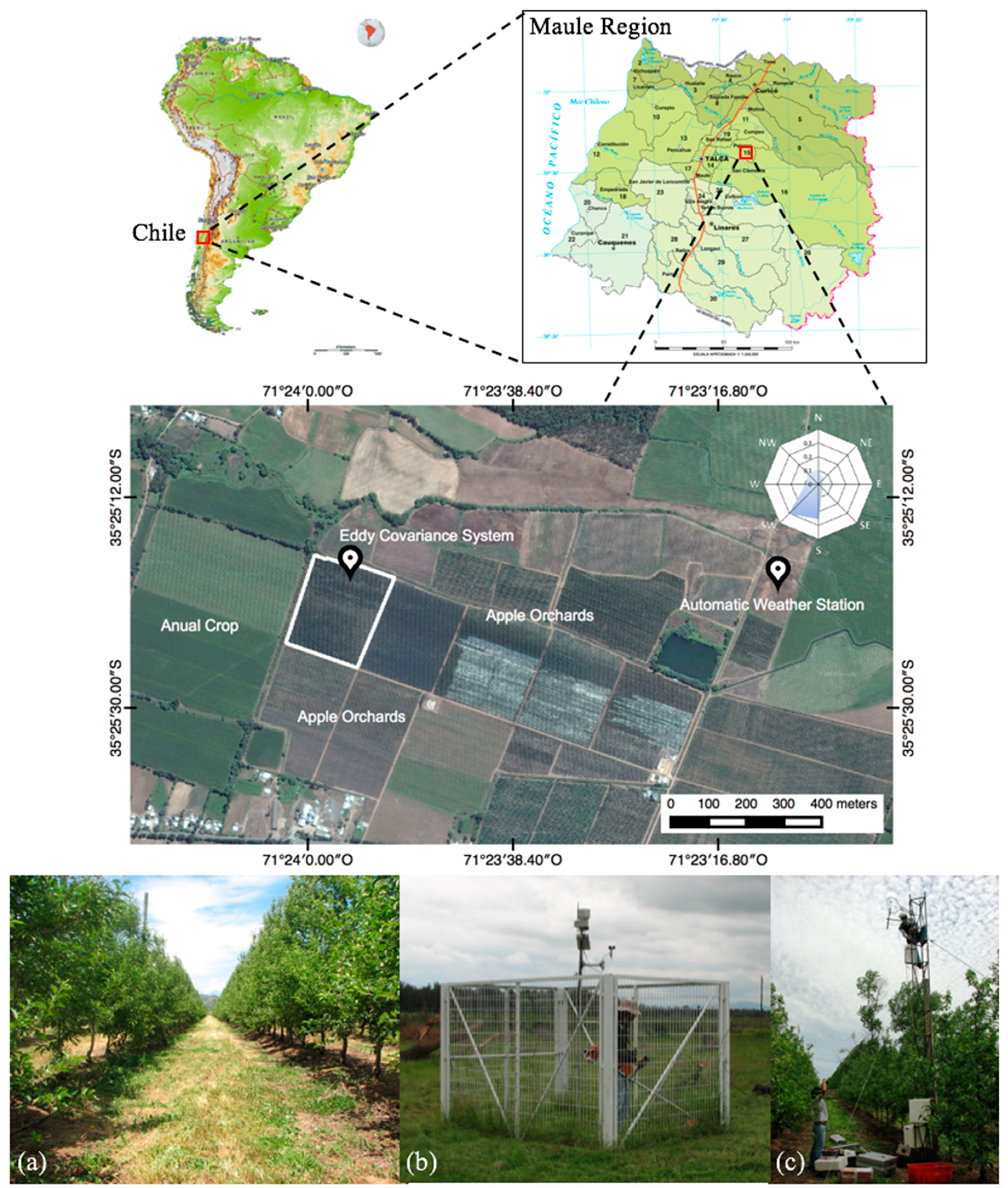
2.1. Study Area

The study was conducted in 5.5 ha of drip-irrigated apple (Malus domestica cv. Pink Lady) orchard located in the Pelarco valley, Maule Region, Chile (35°25′20′′LS; 71°23′57′′LW; 189 m above sea level) (Figure 1) during three growing seasons (2012/2013, 2013/2014 and 2014/2015). The experimental plot was surrounded by other apple fields with similar management and conditions. The climate of the study area corresponds to a typical Mediterranean with a daily average temperature of 14.5 °C between September and March (local spring to summer) and average annual rainfall of 700 mm, concentrated mainly throughout the winter months. The summer period is usually hot (30 °C max.) and dry (3.5% of annual rainfall) with a very high atmospheric demand for water vapor, while the winter is cold (−2 °C min) and wet (74.5% of annual rainfall). The soil at the experimental field is classified as “Pelarco series”, which corresponds to a loamy clay texture on an alluvial terrace position having flat topography (34% clay, 30% silt and 36% sand). For the effective rooting depth (0–90 cm), the average volumetric soil water content at field capacity (θ_FC) and wilting point (θ_WP) were 0.22 m³·m⁻³ (132 mm) and 0.35 m³·m⁻³ (210 mm), respectively.

The apple trees were planted in 2008 with a density of 1667 trees·ha⁻¹ (4.0 × 1.5 m plant spacing) and irrigated daily using drippers (4 L·h⁻¹) spaced at intervals of 0.75 m (Figure 1a). The experimental plot was maintained under non-water stress conditions during the whole season. The trees were trained on a vertical axis system with an average tree height of 4 m and canopy width of 1.55 m. Typical tree trunk diameters ranged between 65 and 79 mm during the three study seasons.

2.2. Plant Measurements

To evaluate the quality of irrigation management, the midday stem water potential (Ψ_md) was evaluated weekly with a pressure chamber (PMS 600, PMS Instrument Company, Corvallis, OR, USA) during the three growing seasons. Fully expanded leaves (two per tree, one tree per replicate) were removed from 18 trees, wrapped in aluminum foil, and encased in a plastic bag at least 2 h before measurement [30]. Measurements were done at midday (12:00–14:00 h) from sunlit leaves situated on both sides of the apple rows. Volumetric soil water content (θ_i) at the rooting depth (0–0.6 m) was monitored weekly at 10 sampling points distributed inside the experimental plot using a portable time domain reflectometry (TDR) unit (TRASE, Soil Moisture Corp., Santa Barbara, CA, USA). LAI was measured biweekly in 20 trees during the study period using a plant canopy analyzer (LAI-2000, LI-COR, Lincoln, NE, USA) with diffuse radiation at sunset. Finally, the plant canopy analyzer was calibrated defoliating 4 trees, where the leaves of each tree were photographed, and then, the total leaf area per tree was measured using a digital image analysis [7,31].

2.3. Weather Data for ETr-PM Estimation

An automatic weather station (AWS) (Adcon Telemetry, A733 GSM/GPRS, Klosterneuburug, Austria) was installed over a well-watered grass at 1000 m to the northeast of the apple orchard to measure the solar radiation (R_s) (W·m⁻²), wind speed (u₂) (m·s⁻¹), relative humidity (RH) (%), and air temperature (T_a) (°C) at 15-min time intervals (Figure 1b). These variables were used as inputs to compute instantaneous (ETr_i) and daily reference evapotranspiration (ETr) using FAO Penman–Monteith equation [2].

2.4. Energy Balance Component Measurements

A tower of 5.5 m height was installed to measure the energy balance components over the drip-irrigated apple orchard (Figure 1c). Latent (LE_E) and sensible (H_E) heat fluxes were measured with an eddy covariance (EC) system, which is composed of a three-dimensional sonic anemometer (CSAT3, Campbell Scientific Inc., Logan, UT, USA) and an infrared gas analyzer (LI-7500, LI-COR Inc., Lincoln, NE, USA). Instantaneous measurements of temperature and humidity were registered at a frequency of 10 Hz and stored on a data logger (CR5000, Campbell Scientific Inc., Logan, UT, USA). The post processing of raw EC data included density correction [32], the sonic temperature correction [33], and coordinate rotation [34].

The net radiation (Rn_E) was measured using a four-way net radiometer (CNR1, Kipp and Zonen Inc., Delft, The Netherlands) and soil heat flux (G_E) was obtained using soil heat flux plates buried at a depth of 0.08 m (HFT3, Campbell Scientific Inc., Logan, UT, USA). In addition, soil temperature was measured by four soil thermocouples (TCAV, Campbell Scientific Inc., Logan, UT, USA) positioned at 0.02 and 0.06 m depth above each heat flux plate [35]. Four plates were installed under tree rows and four other plates were located between rows.

The method proposed by [36] (R92 model) was used to estimate Z_om. In this case, the wind velocities from the CSAT3 and canopy height were used to compute Z_om values over the EC footprint area. Data processing, equations and theoretical basis used in this study are described by [37].

2.5. Data Quality Control and Post-Processing

To reduce the uncertainty associated with error in the LE_E and H_E measurements, entire days were excluded from the study when the ratios of (H_E + LE_E) to (Rn_E − G_E) were outside the range of 0.8 and 1.2 [7]. In addition, H_E and LE_E values were adjusted using the Bowen ratio (β = H_E/LE_E) to close the energy balance for measured fluxes as follows [38,39,40]:

$${\mathrm{H}}_{\beta }=\frac{\beta ·\left({\mathrm{Rn}}_{\mathrm{E}}-{\mathrm{G}}_{\mathrm{E}}\right)}{1+\beta }$$

(9)

$${\mathrm{LE}}_{\beta }=\frac{\left({\mathrm{Rn}}_{\mathrm{E}}-{\mathrm{G}}_{\mathrm{E}}\right)}{1+\beta }$$

(10)

2.6. Satellite Images and Processing Procedure

Twenty Landsat 7 ETM+ satellite images (path 233/row85) were downloaded using the USGS Global Visualization Viewer (GLOVIS, http://glovis.usgs.gov). All scenes used in this research (

Table 1. Summary of Landsat 7 ETM+ satellite imagery used to estimate land surface energy balance fluxes over the apple orchard (path 233/row 85).

	Date	Day of Year (DOY)	Local Acquisition Time	Cloud Cover
Validation set	11 November 2012	316	11:30:22	1%
	27 November 2012	332	11:30:27	1%
	29 December 2012	364	11:30:33	1%
	30 January 2013	30	11:30:40	2%
	15 February 2013	46	11:30:40	1%
	3 March 2013	62	11:30:37	11%
	19 March 2013	78	11:30:34	6%
Calibration set	30 November 2013	334	11:30:46	7%
	16 December 2013	350	11:30:47	4%
	17 January 2014	17	11:31:05	26%
	2 February 2014	33	11:31:21	6%
	18 February 2014	49	11:31:09	2%
	6 March 2014	65	11:31:16	0%
	22 March 2014	81	11:31:26	0%
Calibration set	1 November 2014	305	11:32:28	1%
	17 November 2014	321	11:32:42	16%
	4 January 2015	4	11:33:00	3%
	5 February 2015	36	11:33:10	0%
	21 February 2015	52	11:33:15	11%
	9 March 2015	68	11:33:21	0%

) considered only days having less than 30% cloud cover at the field scale, acquired between November and March. The images had a standard level “Level 1T” correction performed by the USGS, which provides geometric and radiometric correction using ground control points and digital elevation model.

2.7. Calibration of LAI, Z_om and G_i Functions

In general, Z_om, LAI and G_i functions in METRIC were developed for annual crops and may not apply well to heterogeneous or complex canopies such as orchards. In this experiment, the Weibull function was calibrated to estimate LAI as follows (determination coefficient (R²) = 0.87):

$$\mathrm{LAI}=2.42-1.04e^{-502.1·{\mathrm{NDVI}}^{9.32}}$$

(11)

For heterogeneous canopies, the Perrier function [41] has been suggested to estimate Z_om in olive orchards, vineyards and forestry plantations [6,18,23]. The Perrier function is expressed as (R² = 0.82):

$${\mathrm{Z}}_{\mathrm{om}}=\left(\left(1-exp\left(\frac{-a·\mathrm{LAI}}{2}\right)\right)·exp\left(\frac{-a·\mathrm{LAI}}{2}\right)\right)·h$$

(12)

where h (m) is the crop height; a is an adjustment factor describing the LAI distribution within the canopy. In this study, a was 0.06, rather than the standard values of 0.4 to 0.8 [6] due to the impacts of training system and canopy architecture of the apple orchard.

Finally, G_i was computed using the following recalibrated equation:

$$\frac{{\mathrm{G}}_{i\_\mathrm{M}}}{{\mathrm{Rn}}_{i\_\mathrm{M}}}=\mathrm{Ts}·\left(0.0261·\alpha +0.0010\right)·\left(1-0.98·{\mathrm{NDVI}}^4\right)$$

(13)

2.8. Model Validation

The validation of sub-models that compute the instantaneous energy balance components (Rn_i, G_i, LE_i, and H_i), LAI and Z_om is described using the ratio of estimated to observed values (b), mean absolute error (MAE), root-mean-square error (RMSE) and index of agreement (d). The student’s t-test analysis was applied to check whether b was significantly different from unity at the 95% confidence level. Finally, hourly measurements of Rn_i, G_i, H_β and LE_β between 11:00 and 12:00 h (local time) were linearly interpolated to obtain the instantaneous values at the time of the satellite overpass (about 11:30 h). Values of RMSE, MAE and d were respectively computed as [42,43]:

$$\mathrm{RMSE}=\sqrt{\frac{{{\displaystyle \sum }}_{i=1}^i{\left(y_i-y_i\right)}^2}{n}}$$

(14)

$$\mathrm{MAE}=\frac{\left({{\displaystyle \sum }}_{i=1}^i\left|y_i-y_i\right|\right)}{n}$$

(15)

$$d=\left[\frac{{{\displaystyle \sum }}_{i=1}^i{\left(y_i-y_i\right)}^2}{{\displaystyle \sum }\left(\left|y_i\right|+{\left|y_i\right|}^2\right)}\right]$$

(16)

where n is the number of observations, y_i is the observed value, and ŷ_i is the modeled value.

Finally, the model validation was carried out using field data collected during in the 2012/2013 season, while model calibration was carried out using ground-truth data collected during 2013/2014 and 2014/2015 seasons (see Table 1).

3. Results and Discussion

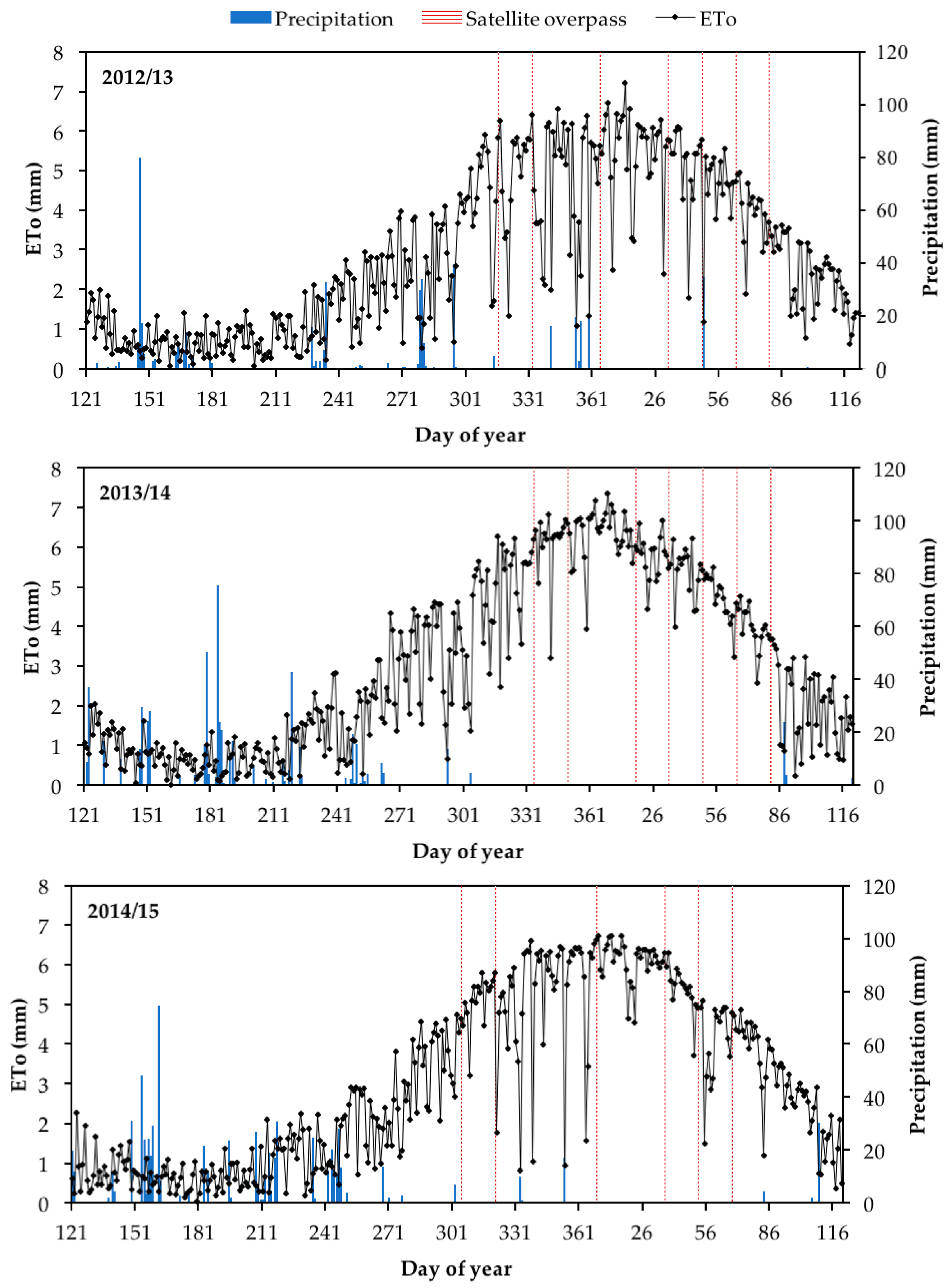
3.1. Climatic and Crop Conditions

Predominantly clear sky days were observed during the three study periods (from November to April) with dry and hot atmospheric conditions. Maximum values for T_a, vapor pressure deficit (VPD) and ETr were observed at satellite overpass time from mid-December to early January (local summer), with means of 28.7 °C (±3.9 °C), 9.1 kPa (±3.8 kPa), and 6.1 mm·day⁻¹ (±0.9 mm·day⁻¹), respectively. Cumulative ETr from September to April ranged between 829 and 904 mm with a maximum value observed during 2013/2014 season. Annual rainfall was mainly concentrated from May to September and totaled 585, 601, and 707 mm for the 2012/2013, 2013/2014 and 2014/2015 study periods, respectively, with no rainfall events near the time of satellite overpasses (Figure 2). The volumetric soil water content at rooting depth and Ψ_md ranged between 0.24 and 0.33 m³·m⁻³, and −1.01 and −1.37 MPa, respectively, indicating that the high-density apple orchard was not under water stress conditions during the three study periods [44].

The energy balance closure for hourly flux measurements is indicated in Figure 3 which shows that many observations were close to the 1:1 line. Statistical analyses indicated that the slope of the regression line through the origin was statistically different from unity at the 95% confidence level, and suggested that turbulent fluxes (H_E + LE_E) were less than the available energy (Rn_E − G_E) by about 14%. According to several researchers, this result is considered appropriate to provide accurate estimates of H_E + LE_E, especially following adjustment using Equations (9) and (10) [45,46,47,48,49].

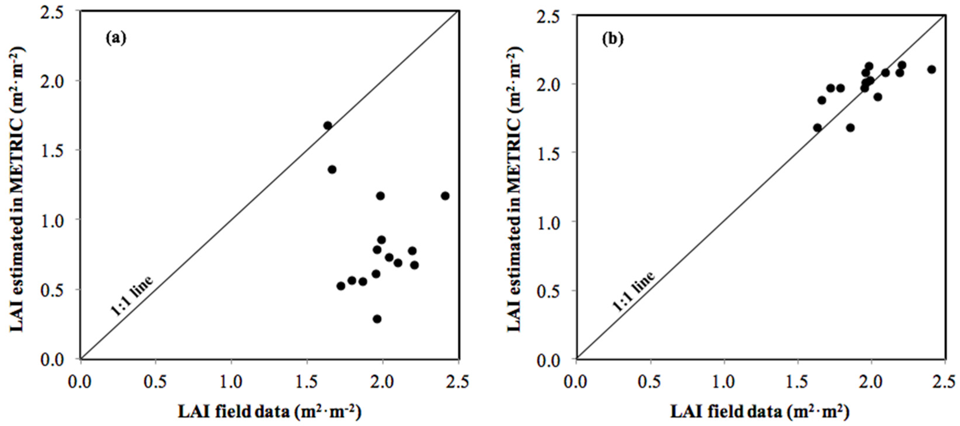
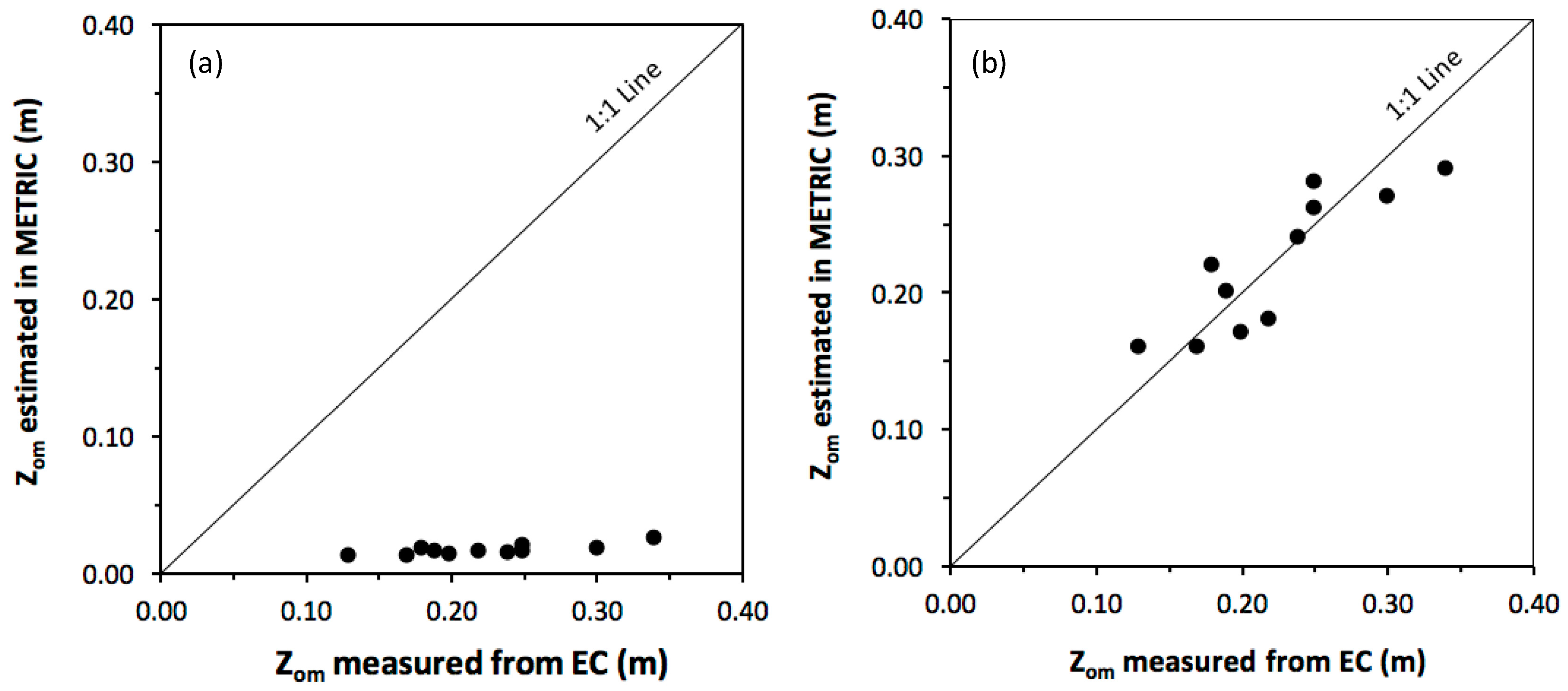
3.2. Validation of the Original and Calibrated Sub-Models of LAI and Z_om

In this study, LAI measured in the apple orchard ranged between 1.65 and 2.41 m²·m⁻² while LAI estimated from original standard equations in METRIC (Equations (4) and (5)) ranged between 0.28 and 1.66 m²·m⁻². Results indicated that the calibrated Weibull model (Equation (11)) estimated LAI with RMSE = 0.2 m²·m⁻², MAE = 0.15 m²·m⁻², and d = 0.44 (

Table 2. Statistical analysis results from recalibrated sub-models to estimate leaf area index (LAI), momentum roughness length (Z_om), net radiation (Rn_i), soil heat flux (G_i), sensible heat flux (H_i), and latent heat flux (LE_i) by the METRIC model over the high-density apple orchard for the 2012/2013 growing season, Pelarco Valley, Chile.

Using Recalibrated LAI, Zom and Gi Algorithms of METRIC
Variable	RMSE	MAE	b	d	t-test
LAI vs. LAIw	0.20 (m2·m-2)	0.15 (m2·m−2)	0.98	0.44	T
Zom vs. Zom_i	0.03 (m)	0.03 (m)	0.94	0.91	T
RnE vs. Rni	19 (W·m−2)	18 (W·m−2)	1.02	0.97	T
GE vs. GC	16 (W·m−2)	14 (W·m−2)	0.97	0.84	F
Hβ vs. Hi	33 (W·m-2)	26 (W·m−2)	1.05	0.16	F
LEβ vs. LEi	30 (W·m−2)	20 (W·m−2)	1.16	0.87	F

RMSE = root mean square error; MAE = mean absolute error; d = index of agreement; b = slope between estimated/observed T = true hypothesis (b = 1); F = false hypothesis (b ≠ 1). Subscripts: “_i” indicated instantaneous values computed by METRIC model, “_E” is measured by the Eddy covariance system, “_β” denotes fluxes corrected by Bowen ratio, “_w” is computed by Weibull calibrated function and “_C” denotes calibrated coefficients, respectively.

). In addition, the t-test indicated that b was significantly equal to unity indicating that estimated and observed values of LAI were similar. In contrast, the original approaches (Equations (4) and (5)) underestimated LAI by about 59% with RMSE and MAE equal to 1.24 and 1.16 m²·m⁻², respectively (

Table 3. Statistical analysis results from the original sub-models to estimate leaf area index (LAI), momentum roughness length (Z_om), net radiation (Rn_i), soil heat flux (G_i), sensible heat flux (H_i), and latent heat flux (LE_i) by the METRIC model over the high-density apple orchard for the 2012/2013 growing season, Pelarco Valley, Chile.

Using Original LAI, Zom and Gi Algorithms of METRIC
Variable	RMSE	MAE	b	d	t-test
LAI vs. LAIM	1.24 (m2·m−2)	1.16 (m2·m−2)	0.41	0.16	F
Zom_E vs. Zom_i	0.22 (m)	0.21 (m)	0.17	0.30	F
RnE vs. Rni	15 (W·m−2)	15 (W·m−2)	1.02	0.98	T
GE vs. Gi	33 (W·m−2)	23 (W·m−2)	1.12	0.74	F
Hβ vs. Hi	95 (W·m−2)	80 (W·m−2)	0.71	0.13	F
LEβ vs. LEi	95 (W·m−2)	81 (W·m−2)	1.26	0.38	F

RMSE = root mean square error; MAE = mean absolute error; d = index of agreement; b = slope between estimated/observed T = true hypothesis (b = 1); F = false hypothesis (b ≠ 1). Subscripts: “_i” indicated instantaneous values computed by METRIC model “_M” is computed by original METRIC model, “_E” is measured by the Eddy covariance system and “_β” denotes fluxes corrected by Bowen ratio, respectively.

). In this regard, Figure 4 indicates that all points from the original standard algorithms were below the line 1:1 while those from the calibrated Weibull model were close to the 1:1 line. Some of the underestimation by the standard functions was due to the tall, narrow nature of the pruned apple trees, where NDVI and SAVI from the nadir-viewing Landsat satellite underestimated actual LAI. Carrasco-Benavides et al. (2014) [18] showed that the performance of the Weibull model depends on the shape of the canopy, fractional cover, and cover crop maintained between rows. In this study, a constant value of fraction cover (0.35 ± 0.03) was observed and the soil surface between rows was kept without weeds, especially from December to March. Major disagreements between observed and estimated values of LAI were found during mid spring (November) when the soil surface between rows was partially covered by weeds. Under this condition, values for NDVI and SAVI were overestimated because satellite images (30 m resolution) failed to represent only orchard cover. Hall et al. (2008) [50] described how the moderate spatial resolution from satellites (such as Landsat) produce mixed-pixel information for vineyards that includes both row and inter-row space information. Agreement between observed and estimated LAI improved after early December when weeds were cut and the soil surface between rows became dry. Finally, the wetted area of the drip-irrigated orchard was only about 5.0% of the total area and was located below the tree canopy.

This study indicates that the calibrated Perrier equation (Equation (12)) using a = 0.06 was able to predict Z_om with RMSE and MAE both equal to 0.03 m (Table 2). In addition, b was significantly equal to unity, indicating that estimated and observed values for Z_om were similar. Furthermore, the original standardized equation (Equation (8)) underestimated Z_om by about 83% with RMSE = 0.22 m and MAE = 0.21 m (Table 3). Figure 5 shows that the estimates by the Perrier equation are close to the 1:1 line when a = 0.06, but those for the standard model setting (a = 0.6) were below the straight line. These results are similar to those found by [18] who indicated that Z_om was underestimated by about 81% when the original function setting was applied to a drip-irrigated vineyard. For ETa estimation from a non-irrigated olive orchard, Santos et al. (2012) [23] found that the implementation of the Perrier function reduced the values of RMSE from 1.12 mm·day⁻¹ to 0.25 mm·day⁻¹. In addition, Pôças, et al. (2014) [22] observed that the Perrier equation applied on a dense hedgerow olive orchard produced similar results to those found in this study where Z_om values varied with LAI and canopy height. These authors also indicated that original equation settings utilized in METRIC for computing Z_om (Equation (8)) tend to produce an underestimation on H_i in the orchard.

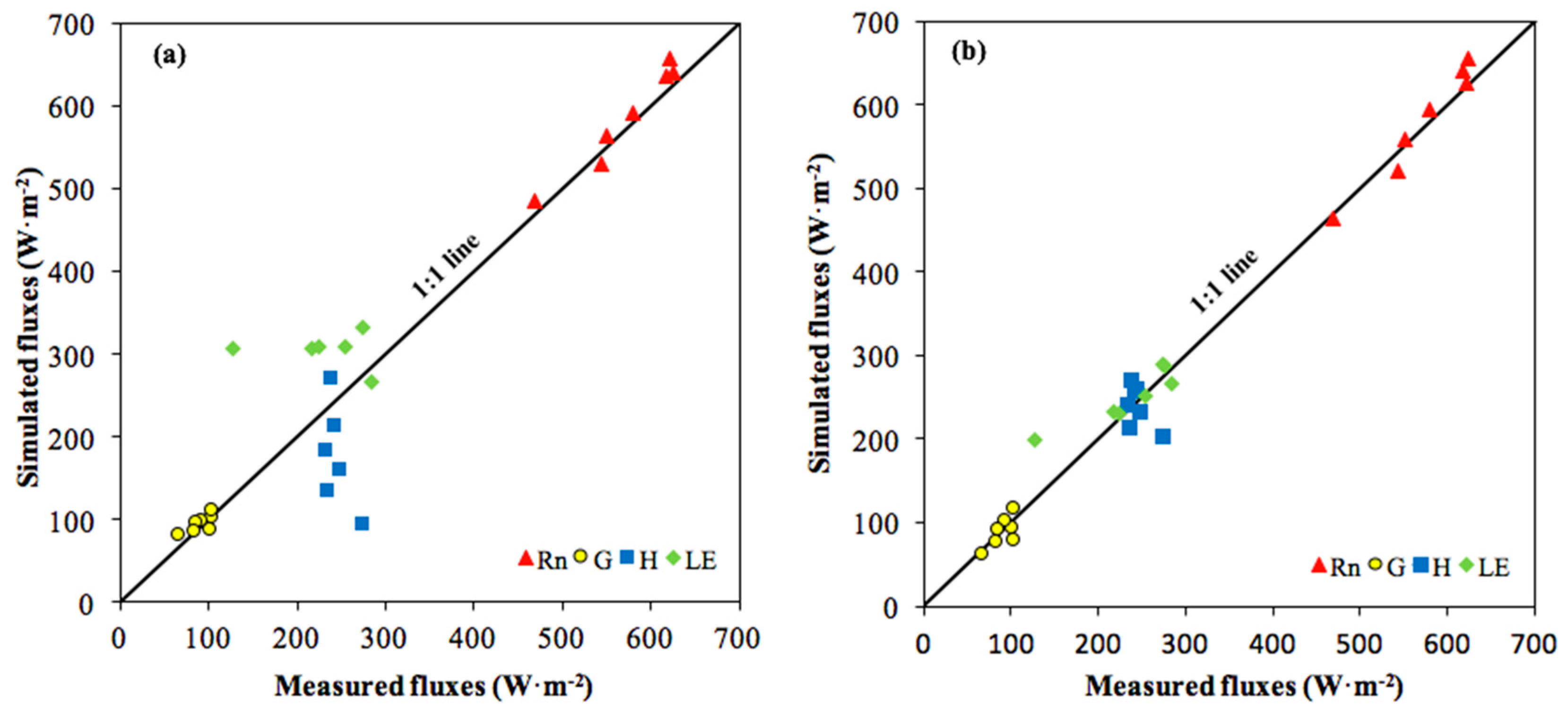
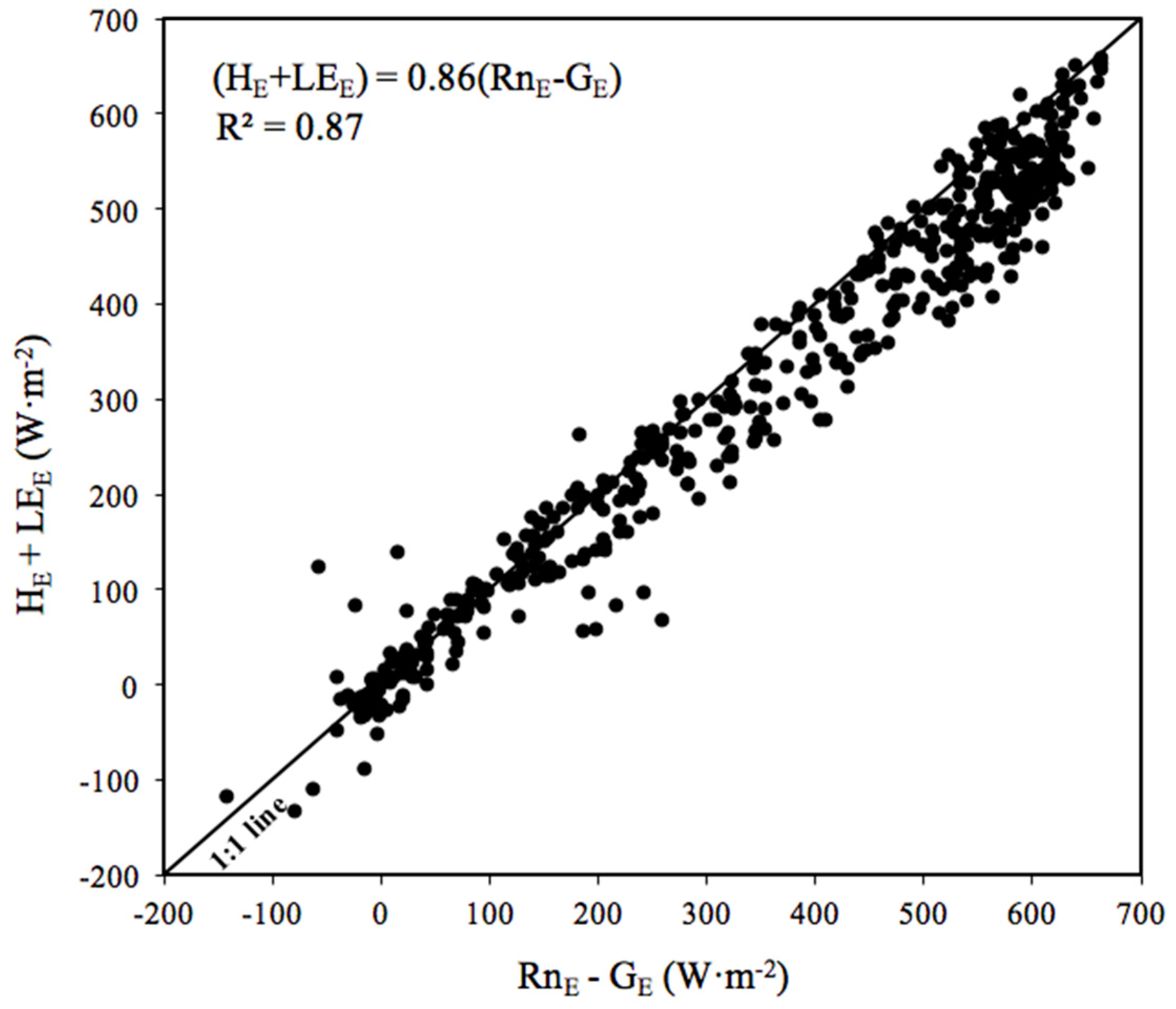
3.3. Validation of Orchard Energy Balance Fluxes

The comparisons between observed and estimated values for LE_i, Rn_i, H_i and G_i at the time of satellite overpasses (11:30–11:40 h local time) are depicted in Figure 6a,b when using the original and calibrated sub-models to compute Z_om, LAI and G_i, respectively. For net radiation (triangles), these figures show that all points were close to the 1:1 line, with RMSE and MAE ranging 15–20 and 15–18 W·m⁻², respectively (Table 2 and Table 3). For both original and calibrated sub-models, the t-test indicated that b was not different from unity (one) indicating that observed and estimated values of Rn_i were similar. In this study, a variation of ±50% in the estimation of LAI produced differences of ±3% in the calculation of broad-band surface emissivity (ε_o = 0.95 + 0.01 LAI) which is used to estimate the outgoing long-wave radiation (Equation (2)). This sensitivity analysis explains why the calibrated version of Weibull approach did not improve the calculation of Rn_i.

The comparison between observed and estimated G_i indicates that the calibration of c₁ and c₂ coefficients reduced the error from 12% to 3%. Values for RMSE and MAE were 33 and 23 W·m⁻² for the original model while those were 16 and 14 W·m⁻² for the calibrated function, respectively. In addition, Figure 6a,b shows that the points were grouped around the 1:1 line. Carrasco-Benavides et al. (2014) [18] and Samani and Bawazir (2015) [51] suggested that error in the estimation of G_i can be associated with the different measurement scales between satellite data and ground-based observations and sun angle.

Results indicated that METRIC using the original, standard functions underestimated H_i by about 29% with RMSE and MAE ranging 80–95 W·m⁻² (Table 3). In this case, Figure 6a shows that points were below the straight line with an important dispersion. When using the calibrated functions for Z_om, METRIC overestimated H_i by about 5% with RMSE = 33 W·m⁻² and MAE = 26 W·m⁻² (Table 2). For these results, Figure 6b shows that points were close to the 1:1 line. In addition, underlying error found in this study may be associated with the selection of the hot pixels which were difficult to define accurately for some satellite scenes. Thus, the internal self-calibration of METRIC (called CIMEC) plays a critical role in achieving accurate values for LE_i because it absorbs many errors and biases generated during the computation of Rn_i and G_i when H_i is estimated [16].

Finally, the statistical analyses indicate that METRIC using the original standard functions was able to simulate LE_i with RMSE and MAE of 95 and 81 W·m⁻², respectively (Table 3). The slope b was statistically greater than one indicating that LE_i was overestimated by about 26%. When using the calibrated functions, METRIC overestimated LE_i over the high-density apple orchard by about 16% with a RMSE = 30 W·m⁻², MAE = 20 W·m⁻² and d = and 0.87 (Table 3). Figure 6 (rhombs) shows that points were closer to the 1:1 when using METRIC with the recalibrated functions for Z_om, LAI and G_i. These results suggest that the calibration of LAI, Z_om, and G_i improved the performance of METRIC to estimate LE_i over the drip-irrigated apple orchard. Allen et al. (2011) [3] indicated that one of the main disadvantages of METRIC is that the accuracy in estimating LE_i for individual pixels depends on errors in the calculations for Rn_i, H_i, and G_i. In general, the smaller the Z_om computed by the original sub-model of METRIC, the lower the values for H_i, and hence estimations of LE_i are typically overestimated. This was the case for the apple orchards. This behavior is particularly important considering that Z_om values are typically underestimated in fruit orchards and vineyards using the standard sub-model parameters (Equation (8)) and consequently the daily actual evapotranspiration is overestimated [23].

Results observed in this study are similar to those found in the literature [18] that indicated that METRIC estimated LE_i with errors of 15% in a drip-irrigated vineyard. González-Dugo et al. (2012) [52] reported an error of 18% in the estimation of LE_i over vine grapes. In an orange orchard, LE_i fluxes computed by a one-source remote sensing model were similar to those measured by an Eddy Covariance system at the field scale, with RMSE equal to 25 W·m⁻² [15]. Usually, the overall mean bias in estimated LE_i and ETa varies between 2% and 25% using one-source models for different fruit crops [53]. These results are considered acceptable by many researchers indicating potential to evaluate different irrigation management with remote sensing techniques and to improve irrigation efficiency at different field scales [6,19,20,54].

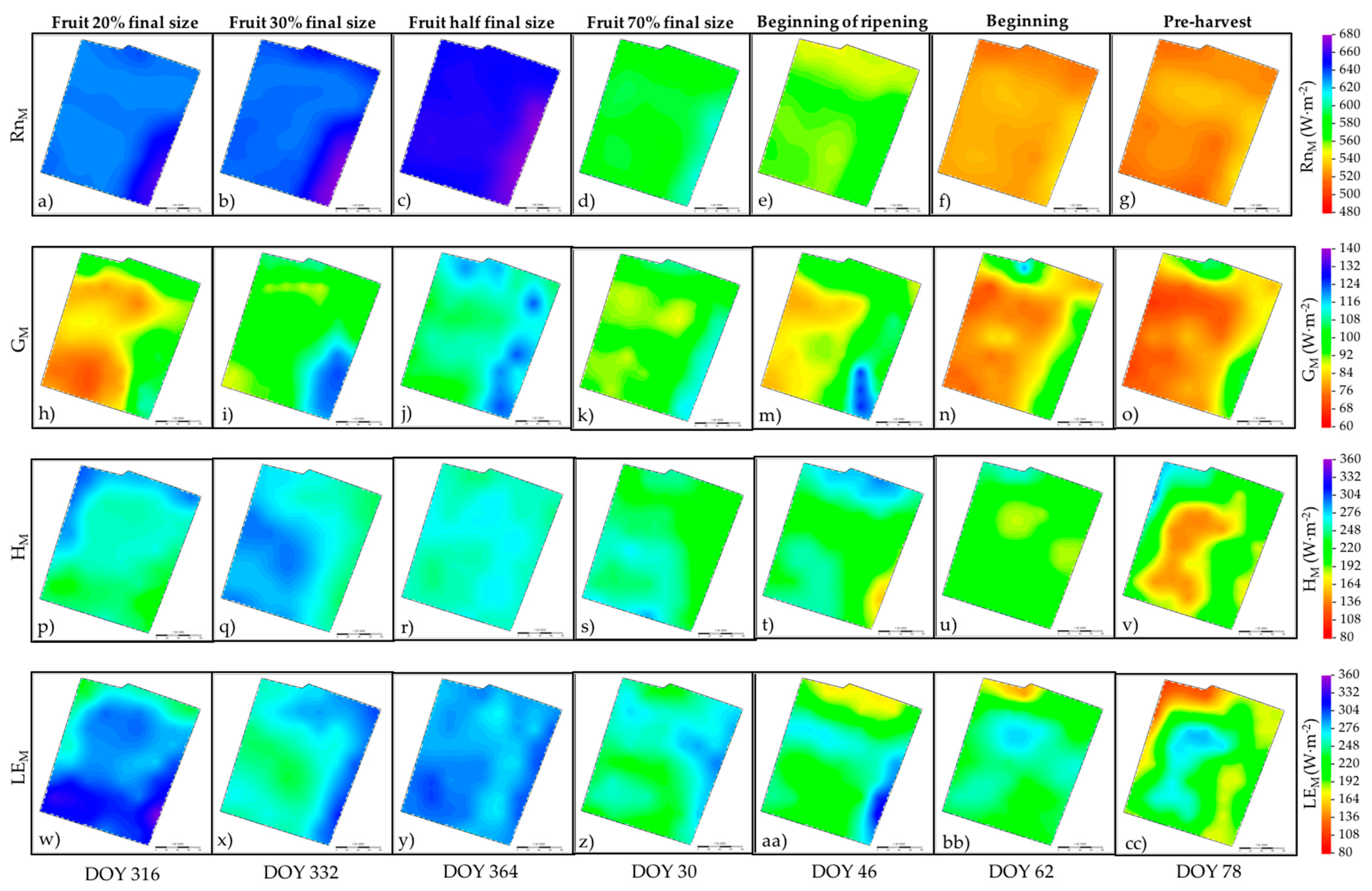
3.4. Distribution of Energy Balance into the Apple Orchard

Maps showing the spatial and temporal variability of the energy balance components over a drip-irrigated apple orchard are illustrated in Figure 7. For the 2012/2013 growing season, the evolution of instantaneous net radiation (Rn_i) (Figure 7a–g), soil heat flux (G_i) (Figure 7h–o), sensible heat flux (H_i) (Figure 7p–v), and latent heat flux (LE_i) (Figure 7w–cc) were computed using METRIC with the calibrated sub-models of Z_om, LAI and G_i. In the study area, mean values for Rn_i ranged between 494 and 636 W·m⁻² with minimum and maximum values observed on DOY 78 and 316, respectively. The spatial variability in Rn_i was quite homogeneous over the apple orchard with a coefficient of variation less than 2% during the study period. Maximum and minimum values for G_i were found on DOY 364 (dry and hot atmospheric conditions) and DOY 78 (beginning of autumn in the southern hemisphere) with average values of 110 (±6) and 82 (±10) W·m⁻², respectively. For G_i, the spatial distribution exhibited a coefficient of variation less than 11% which agreed with changes observed in the scattering during the season. When the fruit reached half of their size (DOY 364), H_i exhibited the highest spatial variability observed over the orchard with mean values of 273 (±44) W·m⁻². In contrast, at the beginning of ripening (DOY46), the lowest spatial variability was detected with mean values of 259 (±3) W·m⁻² and with a coefficient of variation of 3%. Because of the energy balance budget, the spatial variability of LE_i exhibited a coefficient of variation of 4% and 26% for DOY 364 and DOY 46, respectively with mean values of 200 (±52) and 287 (±10) W·m⁻² in each case. At the beginning of the season (DOY 316), the highest values for LE_i were observed in the south side of the plot where a grass cover between rows was growing due to winter rainfall and rising temperatures (mid spring). This condition coincided with maximum differences observed between measured and modeled energy balance fluxes for this day, which led into an overestimation in LE_i by the model. During the pre-harvest period (DOY 78), irrigation water supply was partially suspended in the orchard to predispose fruits and trees for harvest a month later. This issue can be observed as a relatively homogeneous spatial distribution of energy balance components through the orchard, according to the remote sensing analysis.

Application of RSEB models like METRIC to compute orchard water requirements has recently been applied with promising results [22,23]. However, the main limitation of METRIC is that the estimation of LE_i for each pixel is only as accurate as the estimates for Rn_i, G_i and H_i [6]. In this study, the main errors were associated with the selection of hot pixels within the scene which were very difficult to obtain for some satellite images. This limitation may cause significant errors in the computation of LE_i by the model, especially in heterogeneous crops, like grapes and apples, where H could generate a big impact in the orchard energy balance (Equation (1)). In this regard, López-Olivarí et al. (2016) [7] indicated that the canopy architecture (tree density, canopy size, LAI, and fc) and training system can have an important effect in the partitioning of Rn and ETa inside an orchard and in the distribution of the energy balance components over the land surface. In addition, Testi et al. (2004) [48] indicated that the exchange of energy fluxes (Rn_i, G_i, H_i and LE_i) between soil surface and tree canopy is strongly affected by the orchard architecture and its shading, and the sensible heat flux generated at the soil surface can be a major contributor to the energy balance for sparse woody canopies playing a key role in tree transpiration and stomatal closure [55]. However, this issue is not possible to demonstrate accurately in METRIC due to the limitations of one-source models to compute the surface energy balance fluxes using satellite-based blended data of soil and canopy at the 30 × 30 m² pixel size. In addition, main limitations of current satellite platforms for practical application of site-specific irrigation management, especially in heterogeneous canopies such as orchards and vineyards, are the lack of fine spatial resolution and real-time data at the field and sub-field scales [56].

4. Conclusions

METRIC was originally developed to estimate the land surface energy balance and ETa over relatively homogeneous crop canopies, mostly associated with annual crops having full ground cover. However, over sparse woody canopies, standard functions in METRIC tend to produce underestimations for LAI, Z_om and G_i fluxes. This issue generates lower values for H_i and hence high LE_i production via the energy balance budget. After adopting calibrated algorithms for LAI, Z_om, and G_i, the intermediate components of land surface energy balance were adjusted, and error in LAI, G_i and Z_om values over the apple orchard was substantially reduced.

Results suggest that METRIC can be used as an effective tool to simulate the spatial and temporal variability of energy balance components with relative accuracy for a high-density apple orchard, with error within the range of biases observed by other authors who have studied tree crops. However, it is necessary to conduct more research in additional orchards and with different types of fruit trees in order to analyze the behavior of intermediate algorithms of the model, especially in counties such as Chile were a single Landsat scene (180 km²) contains three different microclimatic conditions: The Andes Mountains, the central valley, and the coastal range. Future research should also consider the implementation of the two-source or three-source energy balance models to analyze the behavior of energy balance components over orchards.

References

1. Allen, R.G.; Pereira, L.S.; Raes, D.; Smith, M. Crop Evapotranspiration—Guidelines for Computing Crop Water Requirements—FAO Irrigation and Drainage Paper 56; FAO: Rome, Italy, 1998. [Google Scholar]
2. Task Committee on Standardization of Reference Evapotranspiration. The ASCE Standarized Reference Evapotranspiration Equation; Report of the ASCE-EWRI; ASCE-EWRI: Kimberly, ID, USA, 2005; p. 147. [Google Scholar]
3. Allen, R.G.; Pereira, L.S.; Howell, T.A.; Jensen, M.E. Evapotranspiration information reporting: I. Factors governing measurement accuracy. Agric. Water Manag. 2011, 98, 899–920. [Google Scholar] [CrossRef]
4. Ortega-Farías, S.; Cuenca, R.; English, M. Hourly Grass Evapotranspiration in Modified Maritime Environment. J. Irrig. Drain. Syst. 1995, 121, 369–373. [Google Scholar] [CrossRef]
5. Ortega-Farías, S.; Irmak, S.; Cuenca, R.H. Special issue on evapotranspiration measurement and modeling. Irrig. Sci. 2009, 28, 1–3. [Google Scholar] [CrossRef]
6. Allen, R.; Irmak, A.; Trezza, R.; Hendrickx, J.M.H.; Bastiaanssen, W.; Kjaersgaard, J. Satellite-based ET estimation in agriculture using SEBAL and METRIC. Hydrol. Process. 2011, 25, 4011–4027. [Google Scholar] [CrossRef]
7. López-Olivarí, R.; Ortega-Farías, S. Partitioning of net radiation and evapotranspiration over a superintensive drip-irrigated olive orchard. Irrig. Sci. 2016, 34, 17–31. [Google Scholar] [CrossRef]
8. Cruz-Blanco, M.; Lorite, I.J.; Santos, C. An innovative remote sensing based reference evapotranspiration method to support irrigation water management under semi-arid conditions. Agric. Water Manag. 2014, 131, 135–145. [Google Scholar] [CrossRef]
9. Anderson, M.C.; Allen, R.G.; Morse, A.; Kustas, W.P. Use of Landsat thermal imagery in monitoring evapotranspiration and managing water resources. Remote Sens. Environ. 2012, 122, 50–65. [Google Scholar] [CrossRef]
10. Karimi, P.; Bastiaanssen, W.G.M.; Sood, A.; Hoogeveen, J.; Peiser, L.; Bastidas-Obando, E.; Dost, R.J. Spatial evapotranspiration, rainfall and land use data in water accounting—Part 2: Reliability of water accounting results for policy decisions in the Awash Basin. Hydrol. Earth Syst. Sci. 2015, 19, 533–550. [Google Scholar] [CrossRef]
11. Karimi, P.; Bastiaanssen, W.G.M. Spatial evapotranspiration, rainfall and land use data in water accounting—Part 1: Review of the accuracy of the remote sensing data. Hydrol. Earth Syst. Sci. 2015, 19, 507–532. [Google Scholar] [CrossRef]
12. Bastiaanssen, W.G.M. Remote Sensing in Water Resources Management: The State of the Art; International Water Management Institute: Colombo, Sri Lanka, 1998. [Google Scholar]
13. Barbagallo, S.; Consoli, S.; Russo, A. A one-layer satellite surface energy balance for estimating evapotranspiration rates and crop water stress indexes. Sensors 2009, 9, 1–21. [Google Scholar] [CrossRef] [PubMed]
14. González-Dugo, M.; Gonzalez-Piqueras, J.; Campos, I.; Balbontin, C.; Calera, A. Estimation of surface energy fluxes in vineyard using field measurements of canopy and soil temperature. Remote Sens. Hydrol. 2012, 352, 59–62. [Google Scholar]
15. Consoli, S.; Vanella, D. Comparisons of satellite-based models for estimating evapotranspiration fluxes. J. Hydrol. 2014, 513, 475–489. [Google Scholar] [CrossRef]
16. Allen, R.G.; Tasumi, M.; Trezza, R. Satellite-Based energy balance for Mapping Evapotranspiration with Internalized Calibration (METRIC)—Model. J. Irrig. Drain. Eng. 2007, 133, 380–394. [Google Scholar] [CrossRef]
17. Allen, R.G.; Trezza, R.; Tasumi, M.; Kjaersgaard, J. METRIC: Mapping Evapotranspiration at High Resolution—Applications Manual for Landsat Satellite Imagery; Version 2.0.8; University of Idaho: Kimberly, ID, USA, 2012. [Google Scholar]
18. Carrasco-Benavides, M.; Ortega-Farías, S.; Lagos, L.; Kleissl, J.; Morales-Salinas, L.; Kilic, A. Parameterization of the satellite-based model (METRIC) for the estimation of instantaneous surface energy balance components over a drip-Irrigated vineyard. Remote Sens. 2014, 6, 11342–11371. [Google Scholar] [CrossRef]
19. Gowda, P.; Chávez, J.; Colaizzi, P.; Evett, S.; Howell, T.; Tolk, J. ET mapping for agricultural water management: Present status and challenges. Irrig. Sci. 2008, 26, 223–237. [Google Scholar] [CrossRef]
20. Liou, Y.-A.; Kar, S. Evapotranspiration estimation with remote sensing and various surface energy balance algorithms—A Review. Energies 2014, 7, 2821–2849. [Google Scholar] [CrossRef]
21. Carrasco-Benavides, M.; Ortega-Farías, S.; Lagos, L.O.; Kleissl, J.; Morales, L.; Poblete-Echeverría, C.; Allen, R.G. Crop coefficients and actual evapotranspiration of a drip-irrigated Merlot vineyard using multispectral satellite images. Irrig. Sci. 2012, 30, 485–497. [Google Scholar] [CrossRef]
22. Pôças, I.; Paço, T.A.; Cunha, M.; Andrade, J.A.; Silvestre, J.; Sousa, A.; Santos, F.L.; Pereira, L.S.; Allen, R.G. Satellite-based evapotranspiration of a super-intensive olive orchard: Application of METRIC algorithms. Biosyst. Eng. 2014, 128, 69–81. [Google Scholar] [CrossRef]
23. Santos, C.; Lorite, I.J.; Allen, R.G.; Tasumi, M. Aerodynamic parameterization of the satellite-based energy balance (METRIC) model for ET estimation in rainfed olive orchards of Andalusia, Spain. Water Resour. Manag. 2012, 26, 3267–3283. [Google Scholar] [CrossRef]
24. Hankerson, B.; Kjaersgaard, J.; Hay, C. Estimation of evapotranspiration from fields with and without cover crops using remote sensing and in situ methods. Remote Sens. 2012, 4, 3796–3812. [Google Scholar] [CrossRef]
25. Mokhtari, M.H.; Ahmad, B.; Hoveidi, H.; Busu, L. Sensitivity analysis of METRIC–Based evapotranspiration algorithm. Int. J. Environ. Res. 2013, 7, 407–422. [Google Scholar]
26. Lu, J.; Tang, R.; Tang, H.; Li, Z.-L. Derivation of daily evaporative fraction based on temporal variations in surface temperature, air temperature, and net radiation. Remote Sens. 2013, 5, 5369–5396. [Google Scholar] [CrossRef]
27. Ortega-Farias, S.; Poblete, C.; Brisson, N. Parameterization of a two-layer model for estimating vineyard evapotranspiration using meteorological measurements. Agric. For. Meteorol. 2010, 150, 276–286. [Google Scholar] [CrossRef]
28. Bastiaanssen, W.G.M. SEBAL-based sensible and latent heat fluxes in the irrigated Gediz Basin, Turkey. J. Hydrol. 2000, 229, 87–100. [Google Scholar] [CrossRef]
29. Singh, R.K.; Irmak, A. Treatment of anchor pixels in the METRIC model for improved estimation of sensible and latent heat fluxes. Hydrol. Sci. J. 2011, 56, 895–906. [Google Scholar] [CrossRef]
30. Poblete-Echeverría, C.; Ortega-Farias, S. Evaluation of single and dual crop coefficients over a drip-irrigated Merlot vineyard (Vitis vinifera L.) using combined measurements of sap flow sensors and eddy covariance system. Aust. J. Vitic. 2013, 19, 249–260. [Google Scholar]
31. Colombo, R.; Bellingeri, D.; Fasolini, D.; Marino, C.M. Retrieval of leaf area index in different vegetation types using high resolution satellite data. Remote Sens. Environ. 2003, 86, 120–131. [Google Scholar] [CrossRef]
32. Webb, E.; Pearman, G.; Leuring, R. Correction of the flux measurements for density effects due to heat and water vapour transfer. Q. J. R. Meteorol. Soc. 1980, 106, 85–100. [Google Scholar] [CrossRef]
33. Schotanus, P.; Nieuwstadt, F.; De Bruin, H. Temperature measurements with a sonic anemometer and its applications to heat and moisture fluxes. Bound. Layer Meteorol. 1993, 26, 81–93. [Google Scholar] [CrossRef]
34. Wilczak, J.; Oncley, S.; Stage, S.A. Sonic anemometer Tilt correction algorithms. Bound. Layer Meteorol. 2001, 99, 127–150. [Google Scholar] [CrossRef]
35. Payero, J.; Neale, C.; Wright, J. Estimating soil heat flux for alfalfa and clipped tall fescue grass. Am. Soc. Agric. Eng. 2005, 21, 401–409. [Google Scholar] [CrossRef]
36. Raupach, M.R. Drag and drag partition on rough surfaces. Bound. Layer Meteorol. 1992, 60, 375–395. [Google Scholar] [CrossRef]
37. Chen, Q.; Jia, L.; Hutjes, R.; Menenti, M. Estimation of aerodynamic roughness length over oasis in the Heihe river basin by utilizing remote sensing and ground data. Remote Sens. 2015, 7, 3690–3709. [Google Scholar] [CrossRef]
38. Martínez-Cob, A.; Faci, J.M. Evapotranspiration of an hedge-pruned olive orchard in semiarid area of NE Spain. Agric. Water Manag. 2010, 97, 410–418. [Google Scholar] [CrossRef]
39. Poblete-Echeverría, C.; Ortega-Farias, S. Calibration and validation of a remote sensing algorithm to estimate energy balance components and daily actual evapotranspiration over a drip-irrigated Merlot vineyard. Irrig. Sci. 2012, 30, 537–553. [Google Scholar] [CrossRef]
40. Twine, T.; Kustas, W.; Norman., J.; Cook, D.; Houser, P.; Meyer, T.; Prueger, J.; Starks, P.; Wesely, M. Correcting eddy-covariance flux underestimates over a grassland. Agric. For. Meteorol. 2000, 103, 279–300. [Google Scholar] [CrossRef]
41. Perrier, A. Land surface processes: Vegetation. In Land Surface Processes in Atmospheric General Circulation Models; Eagelson, P.S., Ed.; Cambridge University Press: Cambridge, UK, 1982; pp. 395–448. [Google Scholar]
42. Mayer, D.G.; Butler, D.G. Statistical validation. Ecol. Model. 1993, 68, 21–32. [Google Scholar] [CrossRef]
43. Willmott, C.J.; Ackleson, S.G.; Davis, R.E.; Feddma, J.J.; Klink, K.M.; Legates, D.R.; O’Donell, J.; Rowe, C.M. Statistics for the evaluation and comparison of models. J. Geophys. Res. 1985, 90, 8995–9005. [Google Scholar] [CrossRef]
44. O’Connell, M.G.; Goodwin, I. Responses of “pink lady” apple to deficit irrigation and partial rootzone drying: Physiology, growth, yield, and fruit quality. Aust. J. Agric. Res. 2007, 58, 1068–1076. [Google Scholar] [CrossRef]
45. Oliver, H.R.; Sene, K.J. Energy and water balances of developing vines. Agric. For. Meteorol. 1992, 61, 167–185. [Google Scholar] [CrossRef]
46. Laubach, J.; Teichmann, U. Surface energy budget variability: A case study over grass with special regard to minor inhomogeneities in the source area. Theor. Appl. Climatol. 1999, 62, 9–24. [Google Scholar] [CrossRef]
47. Kordova-Biezuner, L.; Mahrer, I.; Schwartz, C. Estimation of actual evapotranspiration from vineyard by utilizing eddy correlation method. Acta Hortic. 2000, 537, 167–175. [Google Scholar] [CrossRef]
48. Testi, L.; Villalobos, F.J.; Orgaz, F. Evapotranspiration of a young irrigated olive orchard in southern Spain. Agric. For. Meteorol. 2004, 121, 1–18. [Google Scholar] [CrossRef]
49. Ortega-Farias, S.; Carrasco, M.; Olioso, A.; Acevedo, C.; Poblete, C. Latent heat flux over Cabernet Sauvignon vineyard using the Shuttleworth and Wallace model. Irrig. Sci. 2007, 25, 161–170. [Google Scholar] [CrossRef]
50. Hall, A.; Louis, J.P.; Lamb, D.W. Low-resolution remotely sensed images of wine grape vineyards map spatial variability in planimetric canopy area instead of leaf area index. Aust. J. Grape Wine Res. 2008, 14, 9–17. [Google Scholar] [CrossRef]
51. Samani, A.; Bawazir, S. Improving Evapotranspiration Estimation Using Remote Sensing Technology; Technical Completion Report, Account Number (Index #): 125548; New Mexico Water Resources Research Institute: Las Cruces, NM, USA, 2015; p. 28. [Google Scholar]
52. González-Dugo, M.P.; González-Piqueras, J.; Campos, I.; Andréu, A.; Balbontín, C.; Calera, A. Evapotranspiration monitoring in a vineyard using satellite-based thermal remote sensing. Proc. SPIE 2012. [Google Scholar] [CrossRef]
53. Bastiaanssen, W.G.M.; Pelgrum, H.; Soppe, R.W.O.; Allen, R.G.; Thoreson, B.P.; Teixeira, A.H.d.C. Thermal infrared technology for local and regional scale irrigation analysis in horticultural systems. ISHS Acta Hortic. 2008, 792, 33–46. [Google Scholar] [CrossRef]
54. Kamble, B.; Irmak, A.; Martin, D.L.; Hubbard, K.G.; Ratcliffe, I.; Hergert, G.; Narumalani, S.; Oglesby, R.J. Satellite-Based energy balance approach to assess riparian water use. In Evapotranspiration—An Overview; Alexandris, S.G., Stricevic, R., Eds.; InTech: Rijeka, Croatia, 2013. [Google Scholar]
55. Ortega-Farías, S.; López-Olivarí, R. Validation of a two-layer model to estimate latent heat flux and evapotranspiration in a drip-irrigated olive orchard. Am. Soc. Agric. Biol. Eng. 2012, 55, 1169–1178. [Google Scholar] [CrossRef]
56. Ortega-Farías, S.; Ortega-Salazar, S.; Poblete, T.; Kilic, A.; Allen, R.; Poblete-Echeverría, C.; Ahumada-Orellana, L.; Zuñiga, M.; Sepúlveda, D. Estimation of energy balance components over a drip-irrigated olive orchard using thermal and multispectral cameras placed on a helicopter-based unmanned aerial vehicle (UAV). Remote Sens. 2016, 8, 638. [Google Scholar] [CrossRef]
Figure 1. Location of the study area in the Pelarco valley, Maule Region (Central Chile), with the identification of: (a) the super intensive apple orchard; (b) the automatic weather station; and (c) the Eddy Covariance system.
Remotesensing 09 00670 g001
Figure 2. Daily values of reference evapotranspiration (ETr) and precipitation events (vertical solid lines) over the high-density apple orchard during the study seasons (Pelarco valley, Maule Region, Chile). Satellite overpass dates are indicated as vertical dashed lines.
Remotesensing 09 00670 g002
Figure 3. Hourly turbulent energy fluxes (LEE + HE) vs. available energy fluxes (RnE − GE) from an eddy covariance system located in the high-density apple orchard during the 2012/2013, 2013/2014, and 2014/2015 growing seasons (Pelarco valley, Maule Region, Chile).
Remotesensing 09 00670 g003
Figure 4. Comparison between observed and estimated values of Leaf Area Index (LAI) of drip-irrigated apple orchard (Pelarco Valley, Maule Region, Chile): (a) original short crop function; and (b) calibrated by Weibull function for summer periods.
Remotesensing 09 00670 g004
Figure 5. Comparison between observed and estimated values for Aerodynamic Roughness length (Zom) for a drip-irrigated apple orchard (Pelarco Valley, Maule Region, Chile): (a) original short crop function; and (b) adapted Perrier function.
Remotesensing 09 00670 g005
Figure 6. Comparisons between measured and estimated values for instantaneous latent heat flux (LEi), net radiation (Rni), sensible heat flux (Hi) and soil heat flux (Gi) at the time of satellite overpass (11:30–11:40 h local time) during the 2012/2013 growing season for the apple orchard (Pelarco Valley, Maule Region, Chile): (a) original sub-models; and (b) calibrated sub-models.
Remotesensing 09 00670 g006
Figure 7. Spatial and temporal variability of: instantaneous net radiation (Rni) (ag) soil heat flux (Gi) (ho); sensible heat flux (Hi) (pv); and latent heat flux (LEi) (wcc) computed using calibrated algorithms of METRIC model over the study site at the time of satellite flybys (11:30–11:40 h local time), during the 2012/2013 growing season.
Remotesensing 09 00670 g007