
Detection of Tropical Overshooting Cloud Tops Using Himawari-8 Imagery


1
School of Urban and Environmental Engineering, Ulsan National Institute of Science and Technology, Ulsan 44919, Korea
2
Department of Atmospheric Science, Ewha Woman’s University, Seoul 03760, Korea
*
Author to whom correspondence should be addressed.
Remote Sens. 2017, 9(7), 685; https://doi.org/10.3390/rs9070685
Submission received: 1 June 2017
/
Revised: 30 June 2017
/
Accepted: 1 July 2017
/
Published: 4 July 2017
(This article belongs to the Section Atmospheric Remote Sensing)
Abstract
:Overshooting convective cloud Top (OT)-accompanied clouds can cause severe weather conditions, such as lightning, strong winds, and heavy rainfall. The distribution and behavior of OTs can affect regional and global climate systems. In this paper, we propose a new approach for OT detection by using machine learning methods with multiple infrared images and their derived features. Himawari-8 satellite images were used as the main input data, and binary detection (OT or nonOT) with class probability was the output of the machine learning models. Three machine learning techniques—random forest (RF), extremely randomized trees (ERT), and logistic regression (LR)—were used to develop OT classification models to distinguish OT from non-OT. The hindcast validation over the Southeast Asia and West Pacific regions showed that RF performed best, resulting in a mean probabilities of detection (POD) of 77.06% and a mean false alarm ratio (FAR) of 36.13%. Brightness temperature at 11.2 μm (Tb11) and its standard deviation (STD) in a 3 × 3 window size were identified as the most contributing variables for discriminating OT and nonOT classes. The proposed machine learning-based OT detection algorithms produced promising results comparable to or even better than the existing approaches, which are the infrared window (IRW)-texture and water vapor (WV) minus IRW brightness temperature difference (BTD) methods.
1. Introduction
Overshooting convective cloud Tops (OTs) are a common phenomenon occurring in strong convective storms over tropical land and ocean regions. OTs, also called anvil domes or penetrating tops, are defined as domelike clouds forming above a cumulonimbus cloud top or penetrating tropopause [1]. They form when a rising air parcel in a deep convective cloud penetrates through the equilibrium level (or level of neutral buoyancy) due to the rising parcel’s momentum from strong buoyant updrafts within a thunderstorm. The cumulonimbus clouds with OT can frequently cause severe weather conditions, such as cloud-to-ground lightning, large hail, strong winds, and heavy rainfall [2,3,4,5,6,7,8]. Overshooting deep convective clouds over tropical regions penetrate the tropical tropopause layer and even directly into the lower stratosphere, affecting the budget of heat and constituents [9]. As the effects of OTs on the heat and moisture of the upper troposphere and the lower stratosphere are not yet fully identified [9,10], accurate OT detection and its distribution are crucial to better understand these effects.
Satellite remote sensing data have been used for detecting and monitoring OTs. Researchers have proposed various OT detection methods using visible and/or infrared images. Most of the OT detection models are based on infrared images, since infrared imagery can be utilized regardless of image acquisition time, while visible images are only available during the daytime [11,12,13]. There have been two methods widely used for detecting OTs with infrared images. One method is the dual channel difference approach, which uses the brightness temperature (hereafter Tb) difference between water vapor and window channels, documented as the Water Vapor-InfraRed Window channel Brightness Temperature Difference (WV-IRW BTD) in this study (also known as the Dual Channel Difference method) [14,15,16]. However, the method may be inappropriate, since the horizontal advection of stratospheric water vapor not associated with OTs increases the false alarm of OT detection [16,17]. Furthermore, the threshold used in the method varies depending on the characteristics of the satellite data used, such as spatial resolution and spectral wavelengths [17,18].
To address this limitation, the second method, the InfraRed Window texture (IRW-texture) algorithm, was developed based on the characteristics of OTs that appear as a group of pixels with low Tb [17,19]. The IRW-texture method overcomes the over-detection of OTs in the WV-IRW method, as it does not depend on the water vapor distribution in the lower stratosphere and the Tb of a water vapor absorption band [17]. However, the fixed thresholds used in the IRW-texture method for the characteristics of OTs, such as their size and Tb, would still be insufficient to cover the characteristics of various OT cases [20]. More recently, [21] developed a new satellite-based probabilistic OT detection algorithm, producing OT detection results as the probability of occurrence of OTs. Compared to the previous texture-based method, the probabilistic OT detection approach is relatively less affected by the issue of fixed thresholds, but does require additional processing. In [21], a series of pattern recognition analyses were used to define the anvil cloud extent and assign final OTs with a stepwise rating evaluation method, including a score test, OT shape test, and anvil roundness analysis. Logistic regression was then applied to produce OT probability with numerical weather analysis data. Although the carefully designed processing methods can enhance algorithm performance, the multilevel analyses are time consuming and often produce false alarms. With the rapidly growing volumes of satellite data, a simple but robust detection of OTs is desirable.
The goal of this study is to propose machine learning approaches for binary OT detection (“OT occurrence” vs. “no OT occurrence”) with class probability, which are dedicated for operational use on Himawari-8 satellite data. The key idea is to find rules or patterns to differentiate OT pixels from nonOT, based on the characteristics of various channels and their spatial features. The objectives of this study are: (1) to develop OT detection models based on machine learning methods including Random Forest (RF), Extremely Randomized Trees (ERT), and Logistic Regression (LR), producing OT results as both binary output (i.e., OT or nonOT) and class probability using various input variables related to the characteristics of OT extracted from Himawari-8 infrared imagery; (2) to evaluate the performance of the OT detection models and examine the contributing input variables to OT classification; and (3) to perform hindcast validation of the OT detection models to assess the reliability of the proposed models. While [20] used LR to identify OTs from MODIS data for model development and GOES-14 for model evaluation, we propose here to use machine learning-based algorithms as well as LR to detect OTs from Himawari-8 data. As the Himawari-8 Advanced Himawari Imager (AHI) is a geostationary (GEO) imager, it has higher temporal resolution than sun-synchronous or low earth orbiting (LEO) sensors such as MODIS, and has more channels than existing GEO imagers such as the Geostationary Operational Environmental Satellite (GOES), except for GOES-R/GOES-16 and the Multi-functional Transport Satellites (MTSAT) series. To the best of our knowledge, this is the first study where Himawari-8 data have been used for OT detection. Multiple channels from Himawari-8 data could be useful in providing valuable information about the characteristics of OTs. Since Himawari-8 data were directly used to develop OT detection algorithms in this study, the results demonstrate the applicability of the OT detection algorithms to other planned GEO imagers, such as GOES-R/GOES-16 and GEO-KOMPSAT 2A (GK-2A), that have similar characteristics to Himawari-8.
2. Data
2.1. Himawari-8 Visible and Infrared Imagery
The Himawari-8 satellite is a geostationary meteorological satellite operated by the Japan Meteorological Agency (JMA) (Tokyo, Japan). It has payloads consisting of Earth observing instruments and data collection subsystems. The main instrument, the Advanced Himawari Imager (AHI), contains a total of 16 bands to provide multispectral images with improved specifications compared to previous MTSAT satellite series. To satisfy the demand of various users, the AHI collects data over the Full Disk including the East Asia, SouthEast Asia, Australian, and West Pacific regions every 10 min, the Japan Area every 2.5 min, the Target Area every 2.5 min, and the two Landmark Areas every 0.5 min. We used Himawari-8 full-disk images to analyze the Southeast Asian and Southwest Pacific ocean regions. Himawari-8 band 3 (VIS 0.64 µm) data of 500 m spatial resolution were used to construct OT and nonOT reference datasets along with MODIS VIS imagery. Himawari-8 band 11 (WV 8.6 µm), band 13 (IR 10.4 µm), band 14 (IR 11.2 µm), and band 15 (IR 12.4 µm) data of 2 km spatial resolution were employed to calculate the split window differences that were utilized as input variables (explained in Section 3.2).
2.2. MODIS Visible Imagery
MODIS/Aqua calibrated radiances 5 min. level 1B band 1 data (VIS 0.65 µm of MYD02QKM product) with a spatial resolution of 250 m were used to find OT and nonOT reference regions together with the Himawari-8 VIS images. First, the dates and times of MODIS images were identified with NASA Worldview (https://worldview.earthdata.nasa.gov/) to construct OT and nonOT reference data in various cloud systems over the study area from MODIS granules passing. Then, to remove the “bow-tie” effect of the MODIS scan, all of the MODIS images were remapped to a geographic map projection. The bow-tie effect is a pixel shape distortion caused by the scan geometry of the MODIS sensor and the curvature of the Earth. The pixels at the edges of the swath (i.e., the width that sensors observe) are elongated for the along-track (flight direction) and across-track (scan direction) compared to the pixels near the center of the swath, resulting in an artificial increase of the observing area [22,23].
2.3. Tropopause Temperature from the Numerical Weather Prediction Model
The tropopause temperature data of the Global Forecast System (GFS) produced by the National Centers for Environmental Prediction (NCEP) were compared with the Tb of the OT and nonOT samples. The NCEP GFS is a global numerical weather prediction (NWP) system, which forecasts data in a global 0.5-degree latitude/longitude grid produced with a mathematical forward model that is initialized four times daily (i.e., 00, 06, 12, and 18 UTC forecast cycles). Each of these forecasts generates three-hourly output data containing a variety of atmospheric fields on the model grid. In this study, the GFS 3-hourly tropopause temperature data corresponding to the Himawari-8 imagery were used.
3. Methods
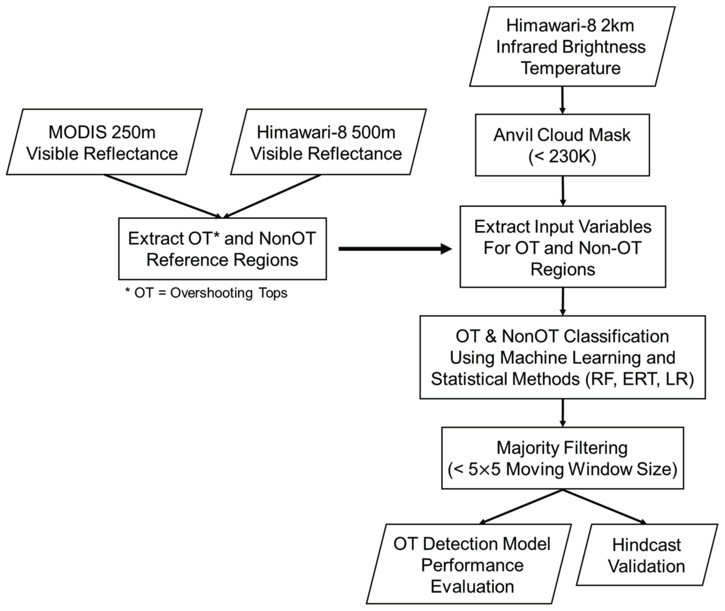
The process flow diagram of the proposed OT detection approach is shown in Figure 1. First, Himawari-8 and MODIS visible images are used to construct the OT and non-OT reference dataset over the Southeast Asia and Southwest Pacific regions for the 1st and 15th day of each month from August 2015 to August 2016 (Section 3.1). Then, a total of 15 input variables were extracted from the Himawari-8 infrared images based on the OT and non-OT reference regions to construct training and test datasets (Section 3.2). Machine learning methods are applied to the training dataset to develop OT classification models with variable importance, and the models are validated using the test dataset (Section 3.3). The three models are applied to other dates of imagery for model prediction with OT classification maps. Finally, accuracy statistics such as probabilities of detection (POD) and false alarm ratios (FAR) are computed for the assessment of the models’ performance.
3.1. Construction of Overshooting Top and Non-Overshooting Top Reference Datasets
The OT and nonOT reference data were constructed with MODIS (250 m) and Himawari-8 (500 m) VIS images by human experts based on visual interpretation. MODIS and Himawari-8 imagery from August 2015 to August 2016 were used as shown in Table 1. As OT signatures are evident in the VIS imagery due to its characteristics, such as shadows cast on the side of the dome-shaped OT clouds and rough surfaces, OTs are identified by human visual interpretation. Akin to earlier works [7,9,20,21], the construction of OT and nonOT reference data was entirely based on the visual interpretation by experts in this study. The images with OT-involved storms were first searched using MODIS VIS data, and these were again examined in the corresponding Himawari-8 VIS images to extract the final OT locations (Figure 2). The nonOT reference data were constructed using the same method. A total of 1076 OT and 2063 nonOT reference data were constructed. About 30% of the constructed OTs were found over the land, and 70% over the ocean. The relative fraction between land and ocean coverages is approximately 40% vs. 60% in the analysis domain. Previous studies reported that land-based convective clouds are stronger than those that occur over the ocean [9,10,24,25]. The studies suggest that the vertical profile of the convective available potential energy (CAPE) can affect the strength of convection. Convection over the land has a wider (fatter) CAPE shape than that over the ocean. Convection in such a wider shape accelerates air parcels more effectively [24]. Another explanation is that the convection can be further strengthened by generating latent heat by the freezing of cloud droplets and raindrops lofted to upper levels. Therefore, convection developing over land disposes of higher aerosol concentrations/content, allowing more water substance to be lofted above the freezing level [25]. Consequently, continental convective clouds generally exhibit stronger vertical velocities, so that the OTs over land were more prominent and better detected than those over the ocean in the previous studies [26].
3.2. Input Variables and Training, Test, and Validation Dataset for Classification of Overshooting Tops
Based on the OT and nonOT reference regions, a total of 15 input variables were extracted, including: (1) the brightness temperature at 11.2 μm (Tb11); (2) its local statistic of standard deviation (STD) at various moving window sizes (MWSs); (3) the Tb11 difference between the center pixel and the average of all the outer-boundary pixels at various MWSs; and (4) the split window differences from the Himawari-8 WV and IR channels (see Table 2). As anvil clouds are identified as regions where cloud pixels with a Tb over 230 K are masked out, the available values in window sizes except for clear sky pixels were used for the calculation of the input variables. Furthermore, the largest window size was 11 × 11 pixels in this study, which means that input variables could not be obtained for the clouds smaller than this window size. Tb11 has different characteristics in the OT and non-OT regions, and it becomes lower toward the center of OT occurrence regions, whereas such changes are not normally significant over non-OT regions. The standard deviation at various MWSs would be useful to discriminate between OT and non-OT regions. Based on the assumption that the differences in Tb11 between the center of a window and its boundary are larger in OT occurrence regions than in non-OT regions, the third set of variables was included in the input variables. Split window differences were first applied for OT detection including 6.2–11.2 µm, 8.6–11.2 µm, 12.4–10.4 µm, and 12.4–11.2 µm from the Himawari-8 data. As a cloud reaches its local equilibrium level or the height of the tropopause, all of the channel differences will be almost zero, and eventually turn positive when an overshooting occurs. The 6.2–11.2 µm difference is used to determine lower stratospheric moisture. It is positive when water vapor is present above the cloud tops (i.e., OTs) [16,27]. The use of 8.6 µm makes the difference more sensitive to small cloud particles, and is useful to detect cloud-top phase transition such as glaciation [13,28]. As the 10.4 µm channel is much less influenced by water vapor than 11.2 µm, it can be more effective for discriminating between clouds with different temperatures than the traditional split window channel (i.e., 11.2 µm) [29]. Eighty percent of the samples were randomly selected and used to train the OT detection models, and the remaining samples were used to validate the models. In addition, the input variables were extracted as a prediction dataset (i.e., for hindcast validation) from the images of different dates to evaluate the ability of model prediction (Table 3).
3.3. Machine Learning Approaches for the Development of Overshooting Top Classification Models
Three machine learning methods—RF, ERT, and LR—were used to develop OT detection models. Machine learning techniques have been widely used in the various applications of satellite remote sensing such as land cover/forest classification and sea ice monitoring in recent years [30,31,32,33,34,35]. The performances of the developed machine learning models was evaluated with the test dataset through confusion matrices. A confusion matrix (or error matrix) is used to summarize the performance of classification models (refer to Tables 4–6 in Results and Discussion). The columns and rows of a confusion table correspond to the classes of reference data and prediction (i.e., classification), respectively. The diagonal elements of the matrix are the number of correctly classified pixels of each class, while the off-diagonal values indicate misclassified pixels. Based on the confusion matrix, the information of producer’s accuracy (PA), user’s accuracy (UA), overall accuracy (OA), and the kappa coefficient values are obtained. PA is calculated as the percentage of correctly classified pixels in terms of all reference pixels. It represents the accuracy of the classification (i.e., omission errors associated with underestimation). UA is calculated as the fraction of correctly classified pixels with regards to all of the pixels categorized as a class. It describes the reliability of classes (i.e., commission errors associated with overestimation). OA is calculated as the total number of correctly classified pixels (i.e., diagonal elements) divided by the total number of pixels in the test data. The Kappa Coefficient of Agreement (hereafter Kappa) is a statistical indicator that measures the degree of agreement between two raters for categorical data. The raters are defined as the reference and predicted data. Kappa can be obtained by calculating the probability of observed agreement in both raters (same as overall accuracy) and the probability that two raters are coincident (i.e., chance agreement). Kappa is a robust statistic, as it considers the likelihood of agreement by chance. In our study, the probability of detection (POD) and the false alarm ratio (FAR) were used for quantitative assessment of the hindcast validation for different dates of imagery that were not used in the training/testing datasets. Region-based POD was applied based on the concept that OT detections that partially occupy the OT reference regions are accepted as correct detections, since the OT reference areas cannot not be fully detected by statistical models [20,26]. The OTs detected within the 11 × 11 MWS of an OT reference center were considered as correct detections [26]. Region-based POD was calculated as follows (Equation (1)).
The FAR was calculated after post-processing that included the pixels immediately adjacent to the correctly detected OT pixels as correct detections. The FAR is calculated based on pixel detections as follows (Equation (2)).
3.3.1. Tree-Based Ensemble Models: Random Forest and Extremely Randomized Trees
RF is composed of multiple independent trees through randomization, and derives its final results through an ensemble method such as voting or weighted voting. RF uses a bootstrap aggregating (Bagging) technique, which constructs multiple sub-datasets through random sampling from the original training dataset with replacement (bootstrapping). RF then aggregates trees constructed by different training datasets (aggregating). RF also uses another randomization, whereby a random subset of input variables is used at each node of trees. In this way, RF tries to generate numerous independent trees to overcome the limitations of the simple decision tree method, such as the dependency on a single tree and sensitivity to training data. RF was implemented using the add-on package of RF in the R statistical program [36]. Default parameter settings were used, including the number of trees (500 as default), the number of variables sampled at each split (sqrt(n) where n is the number of variables), and the minimum node size (1 as default for classification). RF produces the information of mean decrease accuracy (MDA), which measures how much the accuracy decreases when the values of a variable are randomly permuted. The higher the value of MDA of a variable, the more important the variable is to allow distinction between OTs and non-OTs. ERT uses a higher level of randomization than RF, as it applies randomization to the part of optimal splitting in RF, which could also be dependent on the training data [37]. It builds unpruned decision trees, and splits nodes fully at random with the whole learning sample to further reduce the variations between trees. ERT was implemented using the add-on package named “ExtraTrees” in R with default parameters, but does not provide variable importance measures. The tree-based machine learning techniques described above have been widely used in various remote sensing classification and regression applications [38,39,40,41,42,43,44,45,46,47,48,49,50]. Both methods can produce the matrix of class probabilities ranging from 0 to 1 in R. The matrix is calculated as the proportion of vote counts of the trees for each class [51].
3.3.2. Logistic Regression
LR is a regression model that is applied to categorical variables as targets (i.e., dependent variables) to estimate the probability of an event occurrence [23,52,53]. It is similar to linear regression in that the relationship between independent variables and dependent variables is modeled with a specific function that is then used for prediction. Contrary to linear regression, LR is used for classification, as output ranging from 0 to 1 is divided by a fixed threshold by using a logistic (sigmoid) function (Equation (3)).
where P(Y|) is the probability of the dependent variable Y given (), k is the number of independent variables, is the ith independent variable, and is the coefficient for variable . The logistic function estimates the probability of an event (i.e., OT or nonOT). There are three types of LR, binomial LR for a binary dependent variable (i.e., “0” or “1”), multinomial LR for three or more classes, and ordinal LR for three or more classes that are ordered. In this study, binomial LR was implemented in R using the “glm” function. The final results were provided with both probability and binary outputs. In order to create the binary output to classify OT and nonOT results, an optimum threshold was determined using an index called the Critical Success Index (CSI) based on the hindcast validation data along with POD and FAR. The index provides a comprehensive view of POD and FAR, as it is sensitive to correctly classified cases (hits) and simultaneously penalizes misclassifications (misses) and false alarms (Equation (4)).
LR extracts information about the importance of variables using a statistical p-value. The p-value is used to determine whether there is a significant relationship between two variables. The smaller the p-values, the more reliable it is that there is a significant relationship between the two variables. The p-value determines whether a null hypothesis is rejected or not. The null hypothesis is that there is no relationship between two variables. The data used in the experiment should have a p-value of 0.05 or less, which rejects the null hypothesis.
4. Results and Discussion
4.1. Model Performances
The performances of the machine learning models were evaluated using the test dataset (Table 4, Table 5 and Table 6). The RF model showed slightly lower accuracies than ERT, with OTs of 88.94% and 90.03% and kappa coefficients of 0.75 and 0.77, respectively, while the LR model produced the lowest OT and a kappa coefficient of 83.64% and 0.64%. Overall, some OT pixels were missed and misclassified as nonOTs, producing lower accuracies for the OT class. This might be because the sample size of the OT class extracted during the study period was too small to clearly distinguish between OT and nonOT. OT characteristics similar to nonOT in terms of Tb or texture pattern could have caused missed or misclassified results. The biased sample size toward the nonOT class could be another reason, although the ratio of the sample size between OT and nonOT (i.e., 1:2) was chosen based on empirical testing of different ratios (OT:nonOT from 1:1 to 1:5). In addition, the accuracy of the nonOT class is important, as the accurate detection of nonOT can reduce false alarms misclassifying OTs in nonOT regions. OTs were best classified in the ERT model, which had a peak PA of 81.40%, followed by RF with 80.47% and LR with 71.63%. OT regions might have been missed considering the low PAs, as some OT reference pixels were missed by all of the models. The nonOT class was also well captured by the ERT model with a peak PA and UA of 94.38% and 90.97%, respectively. The UAs for the nonOT class were lower than the PAs for all the models, as many OT reference pixels were misclassified as nonOTs, implying an over-detection of nonOTs. Overall, the RF and ERT models produced similar performances for OT and nonOT detection, while the LR model produced lower performance results. All models tended to overestimate nonOTs.
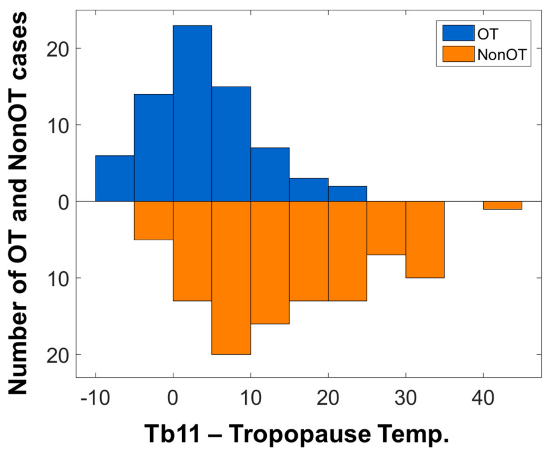
Figure 3 shows the difference between the Tb11 and tropopause temperatures for the OT and nonOT samples of the training and testing data. The Tb11 values of almost all of the nonOT samples are higher than the tropopause temperatures. Some of the OT samples showed lower Tb11 than tropopause temperatures, as the vertical motion of the OTs might have been enough to penetrate through the tropopause. Meanwhile, many of the OT samples are not colder than the tropopause, which implies that not all OT cases occur above the tropopause level, especially in this tropical region where the tropopause level is relatively high. The existing methods developed for the OT cases occurring above the tropopause can miss some OTs that are actually obvious in visible imagery but not colder than the tropopause [19,26].
4.2. Contribution of Input Variables for Overshooting Top Detection
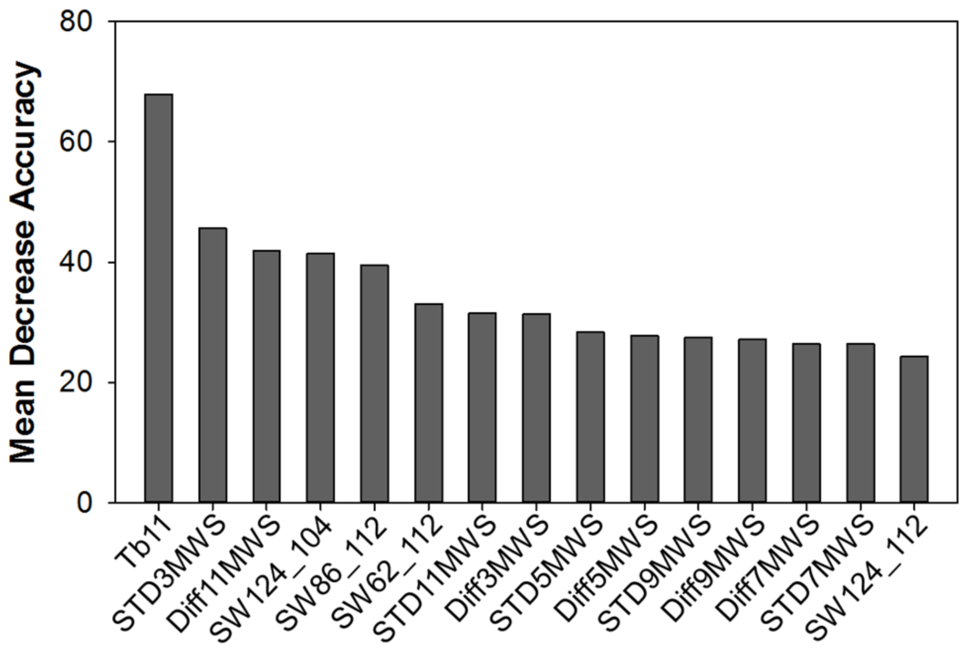
The relative variable importance, identified by the RF and LR models, are shown in Figure 4 and Figure 5, respectively. The Tb11, STD in a 3 × 3 window size (STD3MWS), the difference between the center of the 11 × 11 MWS and its boundary pixels, and the split window differences between 12.4 µm and 10.4 µm (SW124_104), 8.6 µm and 11.2 µm (SW86_112), 6.2 µm and 11.2 µm (SW62_112) were identified as the most contributing variables to OT classification by both models. OTs form at the very top of a thunderstorm with a relatively lower Tb compared to neighboring anvils and non-cumulonimbus clouds, which in turn makes differences in the Tb of OT and non-OT regions in IR bands [20,26,54,55]. As an OT region has a small group of pixels with noticeable temperature gradients relative to anvil cloud regions [7,19,26], OT areas can be distinguished from non-OT regions by using the STD of Tb. STD in a smaller MWS has a higher contribution for OT classification than those in a larger size (i.e., 11 × 11 MWS) for both models. Using an overly large window size does not consider the characteristics of OT regions well when blended with surrounding pixels with various ranges of Tb. The results show that the OTs in this study are effectively highlighted by the 3 × 3 window size. Meanwhile, the Differences variable in the largest window size (11 × 11) ranked higher than those for smaller window sizes. The higher the ranking of a variable, the more important the variable is. The differences in Tb become significant with the increasing distance of the neighboring pixels from the center of OT occurrence regions. As the 10.4 µm channel is less absorbed by water vapor, its split window difference with 12.4 µm contributed more to the discrimination between OT and nonOT than the 12.4–11.2 µm difference [29,56]. The 8.6 µm channel presents cloud-top phase transitions. The stronger vertical velocities of OTs likely result in cloud tops converting their water substance to the ice phase more quickly than in weak updraft [57], making the difference between 8.6 and 11.2 μm an important variable to identify OTs. Since the 6.2 µm channel has been widely used with 11.2 µm for OT detections, in that the Tb in the water vapor band is warmer than in the IR window bands due to the presence of water vapor above OT cloud tops, the 6.2–11.2 µm difference was also identified as a contributing variable [14,16,27]. The broad spectral coverage of Himawari-8 AHI allows for the enhancement of the OT classification.
4.3. Qualitative Evaluation of Overshooting Top Detection Models
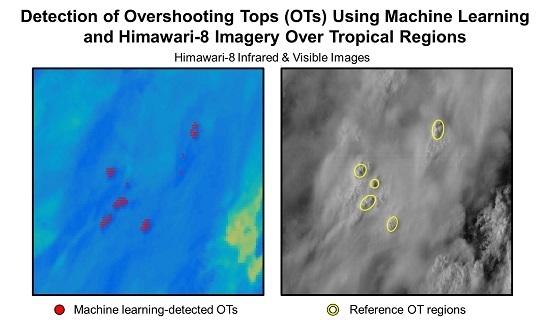
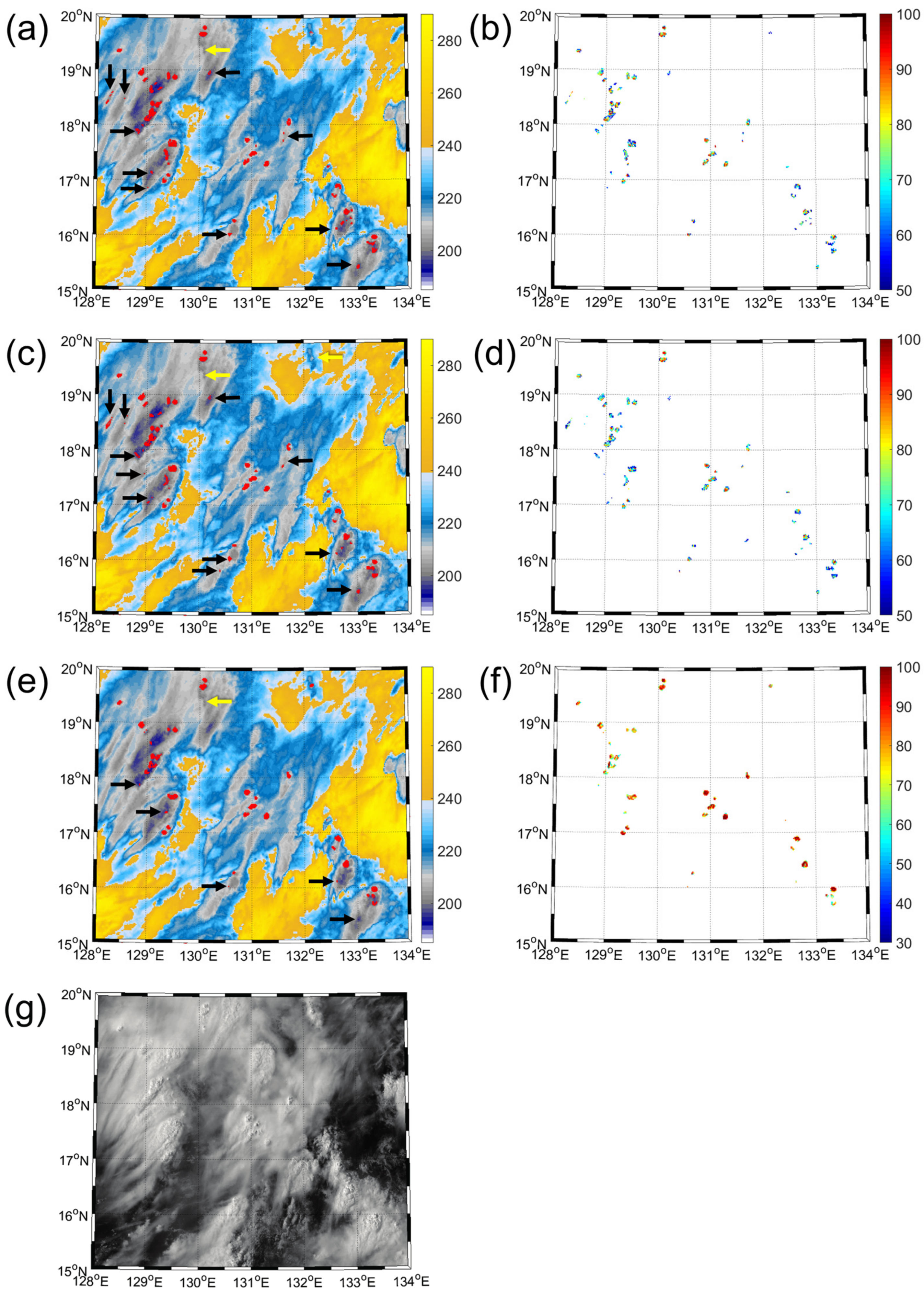
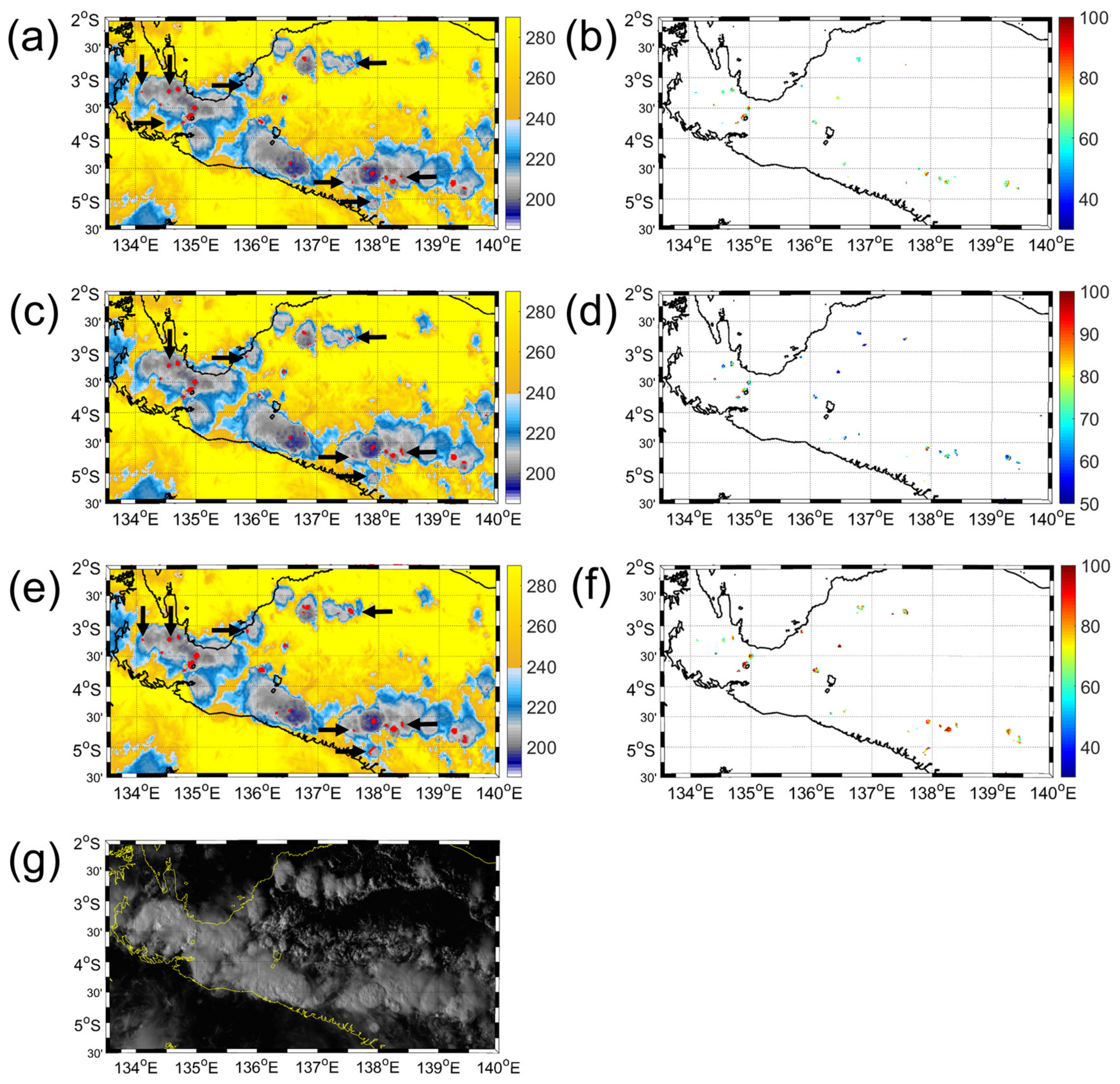
The performance of the LR model using different cut-off thresholds, from 0.1 to 0.9, was tested to determine an optimal threshold for creating a binary OT classification (Figure 6). The optimal threshold was chosen as the average of the thresholds with the highest CSI value for each validation image, which was 0.52. Figure 7 and Figure 8 show the OT detection results for the predicted class (binary) and the class probability of the RF, ERT, and LR models as hindcast validation in a comparison with reference visible imagery. The OT occurrence regions in the VIS images can be easily identified, due to characteristics such as rough surfaces and protrusion over the surrounding anvil clouds, casting shadows on the side of OT clouds [7,54,55,58]. In general, the OT regions in the background IR images have low Tb compared to neighboring clouds. The average difference values in Tb between OT and the surrounding anvil clouds range from approximately −6.61 to −1.33 K by MWS (i.e., Diff11MWS, Diff9MWS, Diff7MWS, Diff5MWS, and Diff3MWS). Though the detection results are slightly different depending on the imagery, the three models show similar detection results overall (Figure 7 and Figure 8). Some falsely detected OT regions (black arrows) were found over anvil cirrus plumes, which are known to generate false alarms [17,21]. As the cirrus clouds have spatial gradients of Tb in IR imagery similar to OTs, some cirrus clouds were misclassified as OT [8]. As discussed in Section 4.1, both tree-based models missed some OT regions (yellow arrows) in Figure 7a,c,e. A possible explanation for this might be that small OT regions could be filtered out by post-processing, or not be detected due to the relatively coarser spatial resolution of Himawari-8’s IR imagery. The right columns of Figure 7 and Figure 8 show the class probability results of RF, ERT, and LR. The higher probabilities are shown in the center of the OT regions. Less than 52% of probabilities were found over anvil cirrus clouds, which represent the nonOT class. The LR model showed slightly better detection results in Figure 7e,f than the other models, while LR resulted in relatively poor performance in Figure 8e,f that produced more false alarms than ERT.
4.4. Quantitative Evaluation of Overshooting Top Detection Models
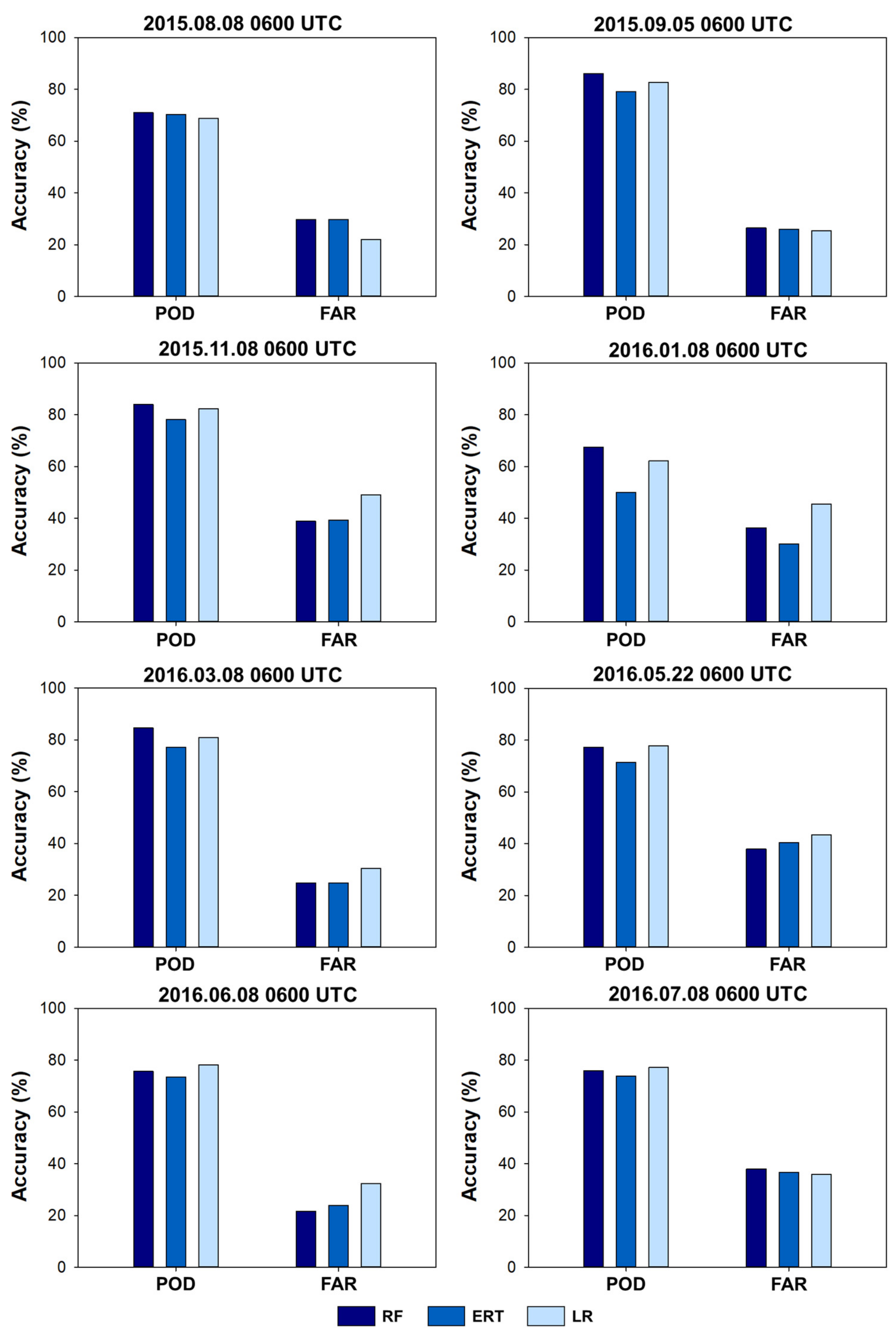
Three models (RF, ERT, and LR) for OT detection were applied to Himawari-8 infrared images (i.e., hindcast validation) that were not used to develop the models. Figure 9 shows the PODs and FARs calculated for Himawari-8 infrared images of eight different dates (Table 3) over the Southeast Asia and Southwest Pacific regions. The three models (RF, ERT, and LR) showed slightly different performances by the date of imagery used. The averaged POD showed similar values for RF and LR, but the RF model has a lower FAR. ERT has a lower POD than the other two models, but its FAR is lower than LR and shows similar performance to RF (Table 7). While RF and ERT showed less variations in FARs with increasing PODs, the FARs in LR greatly increased as the PODs increased, which implies that LR is more sensitive to target imagery compared to the other models. Although ERT performed better than RF in model performance with the testing data, the hindcast validation showed that RF produced better performance in terms of POD and FAR than LR or ERT. Using a total of eight hindscast validation cases for a fairly large tropical area from August 2015 to August 2016, various cloud systems in the tropical regions that result in developing OTs were utilized to evaluate the robustness of the proposed model. Although it is not possible to directly compare our accuracy results with the literature, the accuracies obtained from this present study are comparable to, or even better than, those from the literature: for example, [26] reported a POD of 92.8% and a FAR of 59.9% when using OT pixels not considered to be higher than the tropopause temperature. Bedka and Khlopenkov [21] reported a POD of 69.2% and a FAR of 18.4% or 51.4% (POD) and 1.6% (FAR) depending on two experiments using the logistic regression method. The approaches proposed in this study, particularly the RF model, yielded more accurate validation results, implying that rule-based machine learning approaches are promising for OT detection.
5. Conclusions
In this paper, three machine learning techniques—RF, ERT, and LR—were employed to detect OTs by using various input variables extracted from infrared images. Multiple channels and their derived statistics from the Himawari-8 AHI data were used as input variables in the models. While ERT performed best using the test dataset, RF produced higher PODs and lower FARs than ERT for hindcast validation over the Southeast Asia and Southwestern Pacific regions. The results show that the proposed machine learning-based OT models are relatively simple but robust. Tb11 and STD in a 3 × 3 window size were revealed to be the most contributing variables for discriminating between the OT and nonOT classes. The results agree with the physical characteristics of OT regions, which are low Tb and have a dome-shaped and lumpy surface resulting in large gradients of Tb. Based on the quantitative evaluation results, the machine learning-based OT detection approaches proposed in this study showed similar or even better results compared to the previous studies.
This study is spatiotemporally limited to a year from August 2015 to August 2016 and in the tropical regions. It is thus difficult to directly generalize the proposed models to mid–high latitudinal regions such as East Asia due to different atmospheric and environmental characteristics. Future work should envisage extending spatiotemporal domains, evaluating models more comprehensively in different regions and times. More advanced machine learning methods, such as deep learning (e.g., convolutional neural networks), will be applied for object-based OT detections in future studies to improve the performance of OT detection. The promising results from this present study can allow us to utilize similar approaches to OT detection for planned geostationary satellite sensors such as GOES-R and GK-2A.
Acknowledgments
This work was supported by the “Development of Geostationary Meteorological Satellite Ground Segment (NMSC-2014-01)” program funded by the National Meteorological Satellite Centre (NMSC) of the Korea Meteorological Administration (KMA).
Author Contributions
Miae Kim led manuscript writing and contributed to the data analysis and research design. Jungho Im supervised this study, contributed to the research design and manuscript writing, and served as the corresponding author. Haemi Park, Seonyoung Park, Myong-In Lee, and Myoung Hwan Ahn contributed to the discussion of the results and manuscript writing.
Conflicts of Interest
The authors declare no conflict of interest.
References
- American Meteorological Society. Available online: http://glossary.ametsoc.org/wiki/Overshooting_top (accessed on 28 May 2017).
- Fujita, T.T. Tornado Occurrences Related to Overshooting Cloud-Top Heights as Determined from ATS Pictures; NASA: Chicago, IL, USA, 1972.
- Reynolds, D.W. Observations of damaging hailstorms from geosynchronous satellite digital data. Mon. Weather Rev. 1980, 108, 337–348. [Google Scholar] [CrossRef]
- Negri, A.J.; Adler, R.F. Relation of satellite-based thunderstorm intensity to radar-estimated rainfall. J. Appl. Meteorol. 1981, 20, 288–300. [Google Scholar] [CrossRef]
- Adler, R.F.; Markus, M.J.; Fenn, D.D. Detection of severe midwest thunderstorms using geosynchronous satellite data. Mon. Weather Rev. 1985, 113, 769–781. [Google Scholar] [CrossRef]
- Lane, T.P.; Sharman, R.D.; Clark, T.L.; Hsu, H.-M. An investigation of turbulence generation mechanisms above deep convection. J. Atmos. Sci. 2003, 60, 1297–1321. [Google Scholar] [CrossRef]
- Mikus, P.; Mahović, N.S. Satellite-based overshooting top detection methods and an analysis of correlated weather conditions. Atmos. Res. 2013, 123, 268–280. [Google Scholar] [CrossRef]
- Bedka, K.M. Overshooting cloud top detections using msg seviri infrared brightness temperatures and their relationship to severe weather over Europe. Atmos. Res. 2011, 99, 175–189. [Google Scholar] [CrossRef]
- Takahashi, H.; Luo, Z.J. Characterizing tropical overshooting deep convection from joint analysis of cloudsat and geostationary satellite observations. J. Geophys. Res. 2014, 119, 112–121. [Google Scholar] [CrossRef]
- Liu, C.; Zipser, E.J. Global distribution of convection penetrating the tropical tropopause. J. Geophys. Res. 2005, 110, 37–42. [Google Scholar] [CrossRef]
- Berendes, T.A.; Mecikalski, J.R.; MacKenzie, W.M.; Bedka, K.M.; Nair, U. Convective cloud identification and classification in daytime satellite imagery using standard deviation limited adaptive clustering. J. Geophys. Res. 2008, 113, D20. [Google Scholar] [CrossRef]
- Lindsey, D.T.; Grasso, L. An effective radius retrieval for thick ice clouds using goes. J. Appl. Meteorol. Climatol. 2008, 47, 1222–1231. [Google Scholar] [CrossRef]
- Rosenfeld, D.; Woodley, W.L.; Lerner, A.; Kelman, G.; Lindsey, D.T. Satellite detection of severe convective storms by their retrieved vertical profiles of cloud particle effective radius and thermodynamic phase. J. Geophys. Res. 2008, 113, D4. [Google Scholar] [CrossRef]
- Ackerman, S.A. Global satellite observations of negative brightness temperature differences between 11 and 6.7 µm. J. Atmos. Sci. 1996, 53, 2803–2812. [Google Scholar] [CrossRef]
- Schmetz, J.; Tjemkes, S.; Gube, M.; Van de Berg, L. Monitoring deep convection and convective overshooting with meteosat. Adv. Space Res. 1997, 19, 433–441. [Google Scholar] [CrossRef]
- Setvak, M.; Rabin, R.M.; Wang, P.K. Contribution of the MODIS instrument to observations of deep convective storms and stratospheric moisture detection in goes and msg imagery. Atmos. Res. 2007, 83, 505–518. [Google Scholar] [CrossRef]
- Bedka, K.; Brunner, J.; Dworak, R.; Feltz, W.; Otkin, J.; Greenwald, T. Objective satellite-based detection of overshooting tops using infrared window channel brightness temperature gradients. J. Appl. Meteorol. Climatol. 2010, 49, 181–202. [Google Scholar] [CrossRef]
- Martin, D.W.; Kohrs, R.A.; Mosher, F.R.; Medaglia, C.M.; Adamo, C. Over-ocean validation of the global convective diagnostic. J. Appl. Meteorol. Climatol. 2008, 47, 525–543. [Google Scholar] [CrossRef]
- Proud, S.R. Analysis of overshooting top detections by meteosat second generation: A 5-year dataset. Q. J. R. Meteorol. Soc. 2015, 141, 909–915. [Google Scholar] [CrossRef]
- Dworak, R.; Bedka, K.; Brunner, J.; Feltz, W. Comparison between goes-12 overshooting-top detections, wsr-88d radar reflectivity, and severe storm reports. Weather Forecast. 2012, 27, 684–699. [Google Scholar] [CrossRef]
- Bedka, K.M.; Khlopenkov, K. A probabilistic multispectral pattern recognition method for detection of overshooting cloud tops using passive satellite imager observations. J. Appl. Meteorol. Climatol. 2016, 55, 1983–2005. [Google Scholar] [CrossRef]
- Gomez-Landesa, E.; Rango, A.; Bleiweiss, M. An algorithm to address the MODIS bowtie effect. Can. J. Remote Sens. 2004, 30, 644–650. [Google Scholar] [CrossRef]
- Sayer, A.; Hsu, N.; Bettenhausen, C. Implications of MODIS bow-tie distortion on aerosol optical depth retrievals, and techniques for mitigation. Atmos. Meas. Tech. 2015, 8, 5277–5288. [Google Scholar] [CrossRef]
- Lucas, C.; Zipser, E.J.; Lemone, M.A. Vertical velocity in oceanic convection off tropical Australia. J. Atmos. Sci. 1994, 51, 3183–3193. [Google Scholar] [CrossRef]
- Zipser, E.J. Some views on “hot towers” after 50 years of tropical field programs and two years of trmm data. Meteorol. Monogr. Am. Meteorol. Soc. 2003, 29, 49–58. [Google Scholar] [CrossRef]
- Bedka, K.M.; Dworak, R.; Brunner, J.; Feltz, W. Validation of satellite-based objective overshooting cloud-top detection methods using cloudsat cloud profiling radar observations. J. Appl. Meteorol. Climatol. 2012, 51, 1811–1822. [Google Scholar] [CrossRef]
- Mecikalski, J.R.; Bedka, K.M. Forecasting convective initiation by monitoring the evolution of moving cumulus in daytime goes imagery. Mon. Weather Rev. 2006, 134, 49–78. [Google Scholar] [CrossRef]
- Mecikalski, J.R.; MacKenzie, W.M., Jr.; Koenig, M.; Muller, S. Cloud-top properties of growing cumulus prior to convective initiation as measured by meteosat second generation. Part I: Infrared fields. J. Appl. Meteorol. Climatol. 2010, 49, 521–534. [Google Scholar] [CrossRef]
- Lindsey, D.T.; Schmit, T.J.; MacKenzie, W.M.; Jewett, C.P.; Gunshor, M.M.; Grasso, L. 10.35 μm: An atmospheric window on the goes-r advanced baseline imager with less moisture attenuation. J. Appl. Remote Sens. 2012, 6, 063598. [Google Scholar] [CrossRef]
- Richardson, H.J.; Hill, D.J.; Denesiuk, D.R.; Fraser, L.H. A comparison of geographic datasets and field measurements to model soil carbon using random forests and stepwise regressions (British Columbia, Canada). GISci. Remote Sens. 2017, 54, 573–591. [Google Scholar] [CrossRef]
- Pham, T.D.; Yoshino, K.; Bui, D.T. Biomass estimation of Sonneratia caseolaris (L.) engler at a coastal area of hai phong city (Vietnam) using alos-2 palsar imagery and gis-based multi-layer perceptron neural networks. GISci. Remote Sens. 2017, 54, 329–353. [Google Scholar] [CrossRef]
- Lin, Z.; Yan, L. A support vector machine classifier based on a new kernel function model for hyperspectral data. GISci. Remote Sens. 2016, 53, 85–101. [Google Scholar] [CrossRef]
- Moreira, L.C.J.; Teixeira, A.D.S.; Galvao, L.S. Potential of multispectral and hyperspectral data to detect saline-exposed soils in Brazil. GISci. Remote Sens. 2015, 52, 416–436. [Google Scholar] [CrossRef]
- Kim, M.; Im, J.; Han, H.; Kim, J.; Lee, S.; Shin, M.; Kim, H.-C. Landfast sea ice monitoring using multisensor fusion in the antarctic. GISci. Remote Sens. 2015, 52, 239–256. [Google Scholar] [CrossRef]
- Xun, L.; Wang, L. An object-based svm method incorporating optimal segmentation scale estimation using Bhattacharyya Distance for mapping salt cedar (Tamarisk spp.) with quickbird imagery. GISci. Remote Sens. 2015, 52, 257–273. [Google Scholar] [CrossRef]
- Ihaka, R.; Gentleman, R. R: A language for data analysis and graphics. J. Comput. Gr. Stat. 1996, 5, 299–314. [Google Scholar] [CrossRef]
- Geurts, P.; Ernst, D.; Wehenkel, L. Extremely randomized trees. Mach. Learn. 2006, 63, 3–42. [Google Scholar] [CrossRef]
- Lee, S.; Im, J.; Kim, J.; Kim, M.; Shin, M.; Kim, H.; Quackenbush, L. Arctic sea ice thickness estimation from CryoSat-2 satellite data using machine learning-based lead detection. Remote Sens. 2016, 8, 698. [Google Scholar] [CrossRef]
- Park, S.; Im, J.; Park, S.; Rhee, J. Drought monitoring using high resolution soil moisture through machine learning approaches over the Korean peninsula. Agric. For. Meteorol. 2017, 237, 257–269. [Google Scholar] [CrossRef]
- Gleason, C.J.; Im, J. Forest biomass estimation from airborne LiDAR data using machine learning approaches. Remote Sens. Environ. 2012, 125, 80–91. [Google Scholar] [CrossRef]
- Lee, S.; Han, H.; Im, J.; Jang, E. Detection of deterministic and probabilistic convective initiation using Himawari-8 Advanced Himawari Imager data. Atmos. Meas. Tech. 2017, 10, 1859–1874. [Google Scholar] [CrossRef]
- Long, J.A.; Lawrence, R.L.; Greenwood, M.C.; Marshall, L.; Miller, P.R. Object-oriented crop classification using multitemporal etm+ slc-off imagery and random forest. GISci. Remote Sens. 2013, 50, 418–436. [Google Scholar]
- Han, H.; Lee, S.; Im, J.; Kim, M.; Lee, M.-I.; Ahn, M.H.; Chung, S.-R. Detection of convective initiation using meteorological imager onboard communication, ocean, and meteorological satellite based on machine learning approaches. Remote Sens. 2015, 7, 9184–9204. [Google Scholar] [CrossRef]
- Torbick, N.; Corbiere, M. Mapping urban sprawl and impervious surfaces in the northeast United States for the past four decades. GISci. Remote Sens. 2015, 52, 746–764. [Google Scholar] [CrossRef]
- Park, S.; Im, J.; Jang, E.; Rhee, J. Drought assessment and monitoring through blending of multi-sensor indices using machine learning approaches for different climate regions. Agric. For. Meteorol. 2016, 216, 157–169. [Google Scholar] [CrossRef]
- Park, M.; Kim, M.; Lee, M.; Im, J.; Park, S. Detection of tropical cyclone genesis via quantitative satellite ocean surface wind pattern and intensity analyses using decision trees. Remote Sens. Environ. 2016, 183, 205–214. [Google Scholar] [CrossRef]
- Lu, Z.; Im, J.; Rhee, J.; Hodgson, M.E. Building type classification using spatial attributes derived from LiDAR remote sensing data. Landsc. Urban Plan. 2014, 130, 134–148. [Google Scholar] [CrossRef]
- Ke, Y.; Im, J.; Park, S.; Gong, H. Downscaling of MODIS 1 km Evapotranspiration using Landsat 8 data and machine learning approaches. Remote Sens. 2016, 8, 215. [Google Scholar] [CrossRef]
- Kim, Y.; Im, J.; Ha, H.; Choi, J.; Ha, S. Machine learning approaches to coastal water quality monitoring using GOCI satellite data. GISci. Remote Sens. 2014, 51, 158–174. [Google Scholar] [CrossRef]
- Rhee, J.; Im, J. Meteorological drought forecasting for ungauged areas based on machine learning: Using long-range forecast and remote sensing data. Agric. For. Meteorol. 2017, 237, 105–122. [Google Scholar] [CrossRef]
- Liaw, A.; Wiener, M. Classification and Regression by randomForest. R News 2002, 2, 18–22. [Google Scholar]
- Koutsias, N.; Karteris, M. Burned area mapping using logistic regression modeling of a single post-fire landsat-5 thematic mapper image. Int. J. Remote Sens. 2000, 21, 673–687. [Google Scholar] [CrossRef]
- Nyarko, B.; Diekkruger, B.; van de Giesen, N.; Vlek, P. Floodplain wetland mapping in the White Volta River Basin of Ghana. GISci. Remote Sens. 2015, 52, 374–395. [Google Scholar] [CrossRef]
- Setvak, M.; Lindsey, D.T.; Rabin, R.M.; Wang, P.K.; Demeterova, A. Indication of water vapor transport into the lower stratosphere above midlatitude convective storms: Meteosat second generation satellite observations and radiative transfer model simulations. Atmos. Res. 2008, 89, 170–180. [Google Scholar] [CrossRef]
- Setvak, M.; Bedka, K.; Lindsey, D.T.; Sokol, A.; Charvat, Z.; Stástka, J.; Wang, P.K. A-train observations of deep convective storm tops. Atmos. Res. 2013, 123, 229–248. [Google Scholar] [CrossRef]
- GOES-R ABI Bands Quick Info Guides. Available online: http://www.goes-r.gov/education/ABI-bands-quick-info.html (accessed on 28 May 2017).
- Cintineo, J.L.; Pavolonis, M.J.; Sieglaff, J.M.; Heidinger, A.K. Evolution of severe and nonsevere convection inferred from goes-derived cloud properties. J. Appl. Meteorol. Climatol. 2013, 52, 2009–2023. [Google Scholar] [CrossRef]
- Wang, P.K.; Su, S.-H.; Setvak, M.; Lin, H.; Rabin, R.M. Ship wave signature at the cloud top of deep convective storms. Atmos. Res. 2010, 97, 294–302. [Google Scholar] [CrossRef]
Figure 1.
Data process flow chart proposed in this study. Abbreviations: RF, random forest; ERT, extremely randomized trees; LR, logistic regression.
Figure 1.
Data process flow chart proposed in this study. Abbreviations: RF, random forest; ERT, extremely randomized trees; LR, logistic regression.

Figure 2.
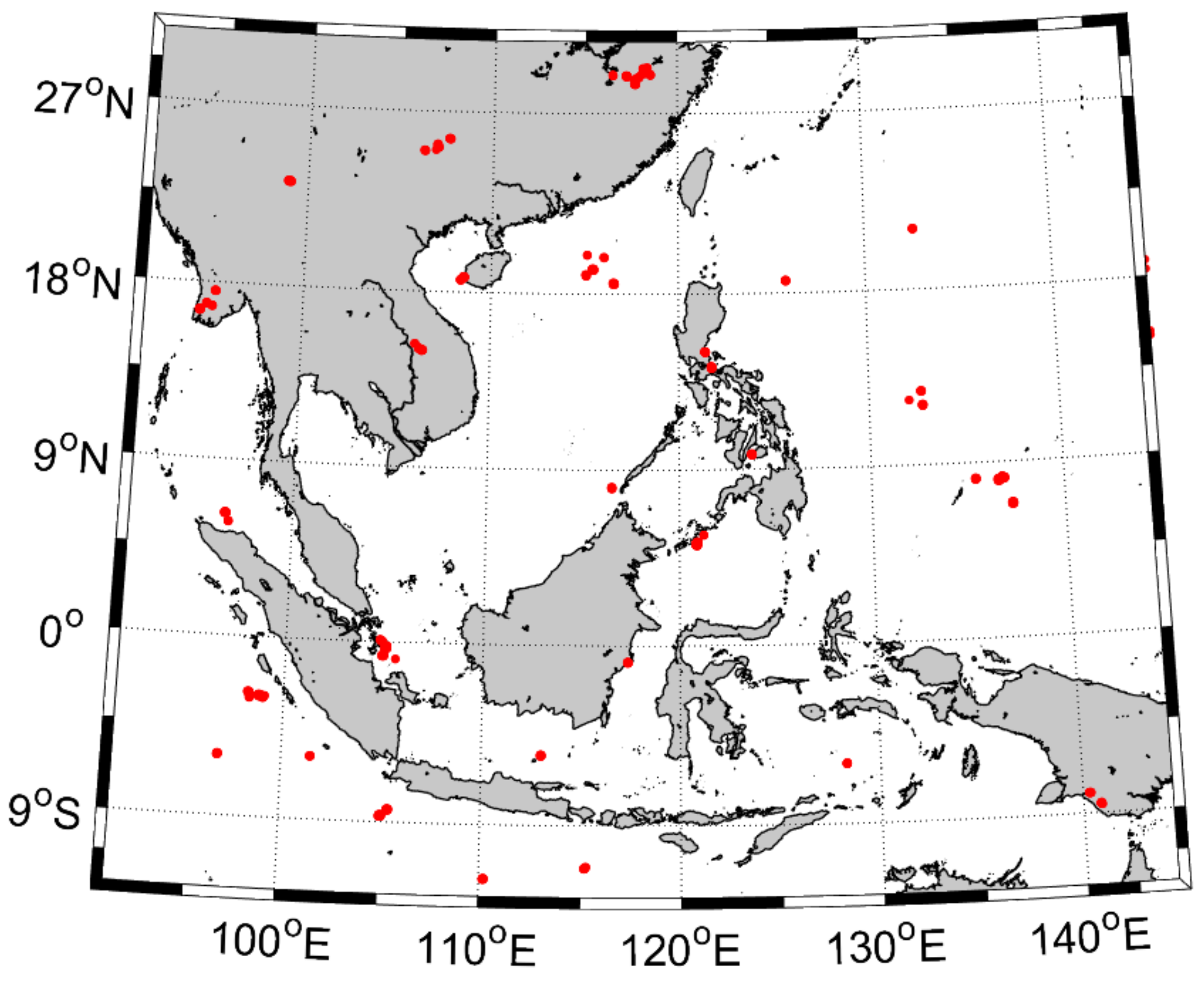
A map of OT reference locations identified by MODIS and Himawari-8 VIS imagery from August 2015 to August 2016 over the Southeast Asia and Southwest Pacific regions. Red dots indicate OT locations, 30.11% of which were found over the land and 69.89% over the ocean.
Figure 2.
A map of OT reference locations identified by MODIS and Himawari-8 VIS imagery from August 2015 to August 2016 over the Southeast Asia and Southwest Pacific regions. Red dots indicate OT locations, 30.11% of which were found over the land and 69.89% over the ocean.

Figure 3.
Difference between the Tb of the Himawari-8 11.2 µm infrared imagery (Tb11) and the tropopause temperatures from numerical weather prediction data for the OT (top) and nonOT (bottom) training and testing data. Note that the lowest Tb pixel per OT/nonOT object was used to make the histogram graph.

Figure 4.
Relative variable importance results by the random forest model. Mean decrease accuracy is calculated using out-of-bag (OOB) data when a variable is permuted. The higher the mean decrease accuracy, the more important the variable is. The definitions of the abbreviations for input variables are shown in Table 2.

Figure 5.
Relative variable importance results indicated by the p-value of the logistic regression model in logarithmic scale. Input variables on the left side of the red vertical line are statistically significant variables with a p-value lower than 0.05. The definitions of the abbreviations for input variables are shown in Table 2.
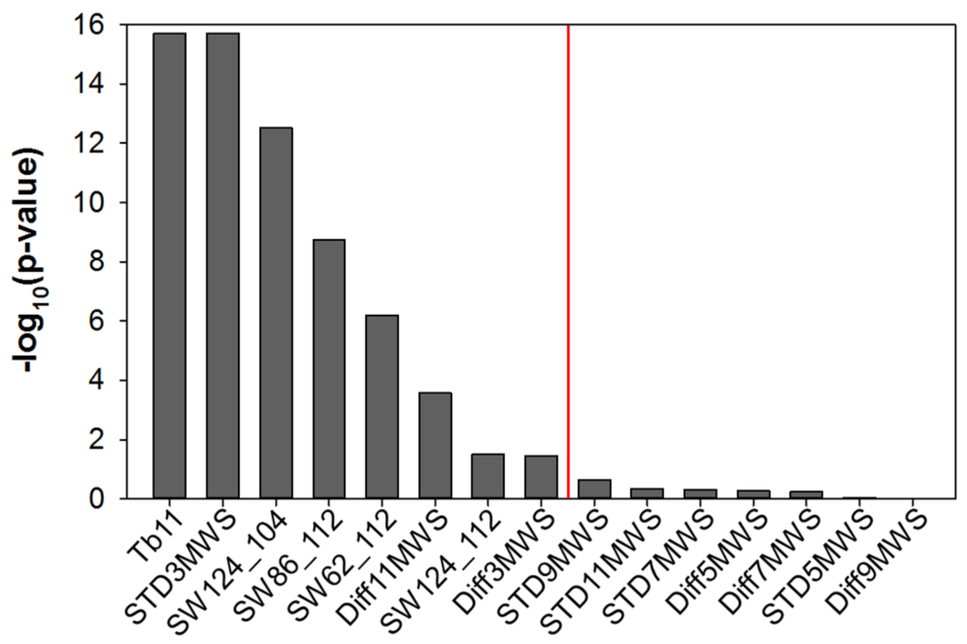
Figure 6.
Validation results with probability of detection (POD)/false alarm ratio (FAR) (left) and critical success index CSI (right) for different cutoff thresholds of the logistic regression model. POD and FAR are expressed as solid and dashed lines, respectively. The average of the thresholds that yield the highest CSI for each case is 0.52, which is indicated by the vertical black line.
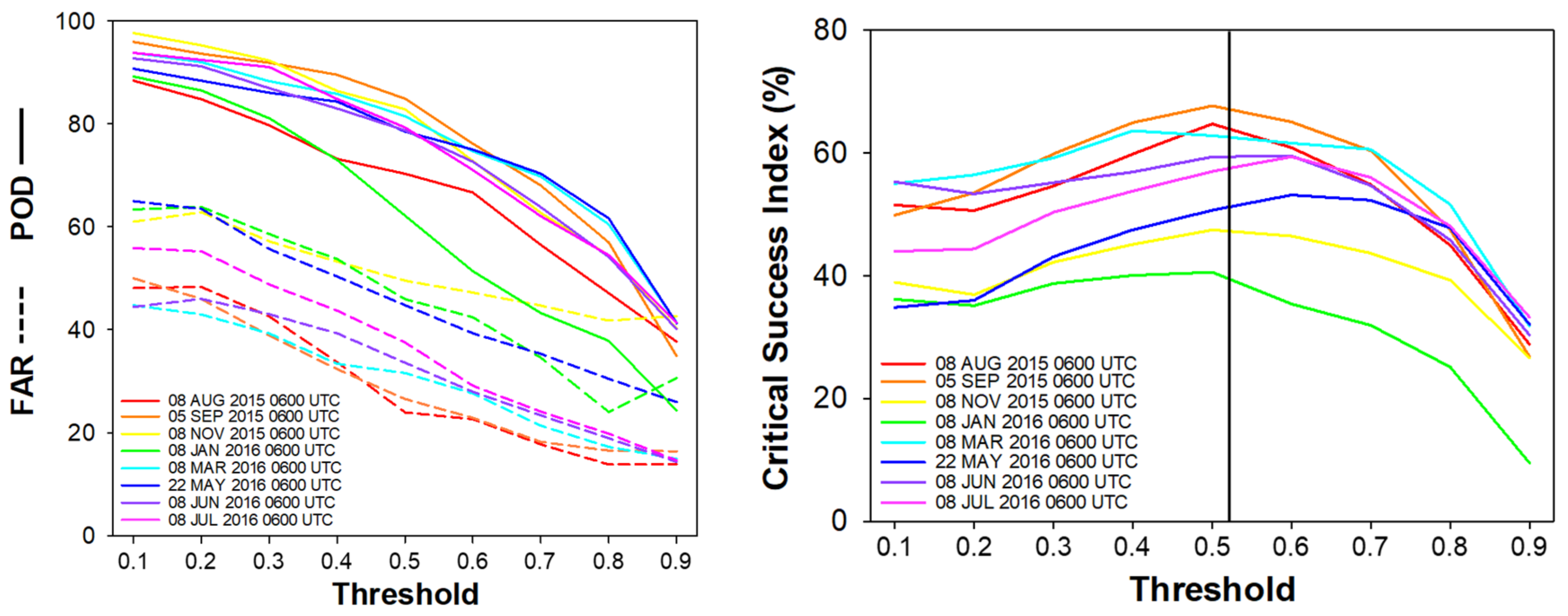
Figure 7.
Overshooting top detection results (red dots) of the (a,c,e) predicted class and the (b,d,f) class probability for random forest (first row), extremely randomized trees (second row), and logistic regression (third row) over selected sub-regions of the Southeast Asia and Southwest Pacific study areas collected at 0600 UTC on 8 August 2015. The background is the 11.2 µm Tb imagery; and (g) visible imagery for the corresponding scene. Falsely detected OTs are shown by black arrows and missed ones by yellow arrows.

Figure 8.
Overshooting top detection results (red dots) of the (a,c,e) predicted class and the (b,d,f) class probability for random forest (first row), extremely randomized trees (second row), and logistic regression (third row) over selected sub-regions of the Southeast Asia and Southwest Pacific study areas collected at 0600 UTC on 8 November 2015. The background is the 11.2 µm Tb imagery; and (g) visible imagery for the corresponding scene. Falsely detected OTs are shown by black arrows and missed ones by yellow arrows.

Figure 9.
Probability of detections (PODs) and false alarm ratios (FARs) for the RF, ERT, and LR models for Himawari-8 infrared images of eight different dates over the Southeast Asia and Southwest Pacific regions.
Figure 9.
Probability of detections (PODs) and false alarm ratios (FARs) for the RF, ERT, and LR models for Himawari-8 infrared images of eight different dates over the Southeast Asia and Southwest Pacific regions.


Table 1.
Information of dates and time of satellite imagery used for constructing OT and nonOT reference dataset.
Table 1.
Information of dates and time of satellite imagery used for constructing OT and nonOT reference dataset.
| Date | Time (UTC) for MODIS | Time (UTC) for Himawari-8 |
|---|---|---|
| 1 August 2015 | 05:10, 05:15 | 05:10 |
| 15 August 2015 | 07:00, 07:05 | 07:00 |
| 1 September 2015 | 06:10 | 06:10 |
| 15 September 2015 | 03:05 | 03:00 |
| 1 October 2015 | 06:20 | 06:20 |
| 15 October 2015 | 03:15 | 03:20 |
| 1 November 2015 | 05:35 | 05:40 |
| 1 December 2015 | 07:25 | 07:30 |
| 1 January 2016 | 06:40 | 06:40 |
| 15 January 20016 | 06:50 | 06:50 |
| 1 February 2016 | 05:55 | 05:50 |
| 15 February 2016 | 06:10 | 06:10 |
| 1 March 2016 | 05:25 | 05:20 |
| 15 March 2016 | 05:40 | 05:40 |
| 1 Aprial 2016 | 06:20 | 06:20 |
| 15 April 2016 | 04:55 | 04:50 |
| 1 May 2016 | 06:35, 06:40 | 06:40 |
| 15 May 2016 | 06:50 | 06:50 |
| 1 June 2016 | 05:55, 06:00 | 06:00 |
| 15 June 2016 | 06:10 | 06:10 |
| 1 July 2016 | 04:25, 04:30 | 04:30 |
| 15 July 2016 | 04:40 | 04:40 |
| 1 August 2016 | 05:20, 05:25 | 05:20 |
| 15 August 2016 | 05:40 | 05:40 |
Table 2.
Summary of the input variables to identify OTs from Himawari-8 Advanced Himawari Imager (AHI) images. The abbreviations are defined in the “List of used variables” column (for example, Diff9MWS means the difference between the center of 9 × 9 moving window size and the mean of its boundary pixels).
| Satellite/Sensor | List of Used Variables (a Total of 15 Input Variables) | Abbreviations | Period | Spatial Resolution |
|---|---|---|---|---|
| Himawari-8/AHI | Tb11 (IR 11.2 µm) | Tb11 | 1st and 15th day of each month from August 2015 to August 2016 | 2 km |
| Standard Deviation (STD) of Tb11 in 3 × 3 moving window size (MWS) | STD3MWS | |||
| STD of Tb11 in 5 × 5 MWS | STD5MWS | |||
| STD of Tb11 in 7 × 7 MWS | STD7MWS | |||
| STD of Tb11 in 9 × 9 MWS | STD9MWS | |||
| STD of Tb11 in 11 × 11 MWS | STD11MWS | |||
| Difference between the center of 3 × 3 MWS and its boundary pixels | Diff3MWS | |||
| Difference between the center of 5 × 5 MWS and its boundary pixels | Diff5MWS | |||
| Difference between the center of 7 × 7 MWS and its boundary pixels | Diff7MWS | |||
| Difference between the center of 9 × 9 MWS and its boundary pixels | Diff9MWS | |||
| Difference between the center of 11 × 11 MWS and its boundary pixels | Diff11MWS | |||
| 6.2–11.2 µm Split Window (SW) difference | SW62_112 | |||
| 8.6–11.2 µm SW difference | SW86_112 | |||
| 12.4–10.4 µm SW difference | SW24_104 | |||
| 12.4–11.2 µm SW difference | SW124_112 |
Table 3.
Information on collection dates and times of satellite imagery used for hindcast validation.
Table 3.
Information on collection dates and times of satellite imagery used for hindcast validation.
| Date | Time (UTC) for Himawari-8 |
|---|---|
| 8 August 2015 | 06:00 |
| 5 September 2015 | 06:00 |
| 8 November 2015 | 06:00 |
| 8 January 2016 | 06:00 |
| 8 March 2016 | 06:00 |
| 22 May 2016 | 06:00 |
| 8 June 2016 | 06:00 |
| 8 July 2016 | 06:00 |
Table 4.
Accuracy assessment result of the random forest model using the test dataset.
| Reference | OT | nonOT | Sum | User’s Accuracy | |
|---|---|---|---|---|---|
| Classified as | |||||
| OT | 173 | 29 | 202 | 85.64% | |
| non-OT | 42 | 398 | 440 | 90.45% | |
| Sum | 215 | 427 | 642 | ||
| Producer’s accuracy | 80.47% | 93.21% | |||
| Overall accuracy | 88.94% | ||||
| Kappa coefficient | 0.75 | ||||
Table 5.
Accuracy assessment result of the extremely randomized trees model using the test dataset.
| Reference | OT | nonOT | Sum | User’s Accuracy | |
|---|---|---|---|---|---|
| Classified as | |||||
| OT | 175 | 24 | 199 | 87.94% | |
| non-OT | 40 | 403 | 443 | 90.97% | |
| Sum | 215 | 427 | 642 | ||
| Producer’s accuracy | 81.40% | 94.38% | |||
| Overall accuracy | 90.03% | ||||
| Kappa coefficient | 0.77 | ||||
Table 6.
Accuracy assessment result of the logistic regression model using the test dataset.
| Reference | OT | nonOT | Sum | User’s Accuracy | |
|---|---|---|---|---|---|
| Classified as | |||||
| OT | 154 | 44 | 198 | 77.78% | |
| non-OT | 61 | 383 | 444 | 86.26% | |
| Sum | 215 | 427 | 642 | ||
| Producer’s accuracy | 71.63% | 89.70% | |||
| Overall accuracy | 83.64% | ||||
| Kappa coefficient | 0.63 | ||||
Table 7.
Summary of the PODs and FARs of RF, ERT, and LR for hindcast validation.
| Date | Accuracy | RF | ERT | LR |
|---|---|---|---|---|
| 8 August 2015 | POD | 71.01% | 70.29% | 68.84% |
| 0600 UTC | FAR | 29.68% | 29.76% | 21.99% |
| 5 September 2015 | POD | 86.05% | 79.07% | 82.72% |
| 0600 UTC | FAR | 26.47% | 26.02% | 25.37% |
| 8 November 2015 | POD | 84.02% | 78.11% | 82.29% |
| 0600 UTC | FAR | 38.84% | 39.33% | 49.07% |
| 8 January 2016 | POD | 67.57% | 50.05% | 62.16% |
| 0600 UTC | FAR | 36.36% | 30.05% | 45.54% |
| 8 March 2016 | POD | 84.57% | 77.16% | 80.86% |
| 0600 UTC | FAR | 24.81% | 24.79% | 30.43% |
| 22 May 2016 | POD | 77.33% | 71.51% | 77.91% |
| 0600 UTC | FAR | 37.97% | 40.42% | 43.39% |
| 8 June 2016 | POD | 75.68% | 73.56% | 78.16% |
| 0600 UTC | FAR | 21.66% | 23.96% | 32.39% |
| 8 July 2016 | POD | 75.86% | 73.79% | 77.26% |
| 0600 UTC | FAR | 38.05% | 36.66% | 35.84% |
| Average | POD | 77.76% | 71.69% | 76.27% |
| FAR | 31.73% | 31.38% | 35.50% |
© 2017 by the authors. Licensee MDPI, Basel, Switzerland. This article is an open access article distributed under the terms and conditions of the Creative Commons Attribution (CC BY) license (http://creativecommons.org/licenses/by/4.0/).
Share and Cite
MDPI and ACS Style
Kim, M.; Im, J.; Park, H.; Park, S.; Lee, M.-I.; Ahn, M.-H. Detection of Tropical Overshooting Cloud Tops Using Himawari-8 Imagery. Remote Sens. 2017, 9, 685. https://doi.org/10.3390/rs9070685
AMA Style
Kim M, Im J, Park H, Park S, Lee M-I, Ahn M-H. Detection of Tropical Overshooting Cloud Tops Using Himawari-8 Imagery. Remote Sensing. 2017; 9(7):685. https://doi.org/10.3390/rs9070685
Chicago/Turabian StyleKim, Miae, Jungho Im, Haemi Park, Seonyoung Park, Myong-In Lee, and Myoung-Hwan Ahn. 2017. "Detection of Tropical Overshooting Cloud Tops Using Himawari-8 Imagery" Remote Sensing 9, no. 7: 685. https://doi.org/10.3390/rs9070685
Note that from the first issue of 2016, this journal uses article numbers instead of page numbers. See further details here.