Article

A Method to Obtain Orange Crop Geometry Information Using a Mobile Terrestrial Laser Scanner and 3D Modeling

by
André F. Colaço
1,*,†,
Rodrigo G. Trevisan
1,
José P. Molin
1,
Joan R. Rosell-Polo
2 and
Alexandre Escolà
2
1
Biosystems Engineering Department, Luiz de Queiroz College of Agriculture, University of São Paulo, 13418-900 Piracicaba, Brazil
2
Department of Agricultural and Forest Engineering, Research Group on AgroICT & Precision Agriculture, Agrotecnio Centre, School of Agrifood and Forestry Science and Engineering, University of Lleida, 25198 Lleida, Spain
*
Author to whom correspondence should be addressed.
Present address: CSIRO, Waite Campus, Locked Bag 2, Glen Osmond, SA 5064, Australia.
Remote Sens. 2017, 9(8), 763; https://doi.org/10.3390/rs9080763
Submission received: 14 June 2017 / Revised: 13 July 2017 / Accepted: 19 July 2017 / Published: 25 July 2017
(This article belongs to the Section Remote Sensing in Agriculture and Vegetation)

Abstract

:
LiDAR (Light Detection and Ranging) technology has been used to obtain geometrical attributes of tree crops in small field plots, sometimes using manual steps in data processing. The objective of this study was to develop a method for estimating canopy volume and height based on a mobile terrestrial laser scanner suited for large commercial orange groves. A 2D LiDAR sensor and a GNSS (Global Navigation Satellite System) receiver were mounted on a vehicle for data acquisition. A georeferenced point cloud representing the laser beam impacts on the crop was created and later classified into transversal sections along the row or into individual trees. The convex-hull and the alpha-shape reconstruction algorithms were used to reproduce the shape of the tree crowns. Maps of canopy volume and height were generated for a 25 ha orange grove. The different options of data processing resulted in different values of canopy volume. The alpha-shape algorithm was considered a good option to represent individual trees whereas the convex-hull was better when representing transversal sections of the row. Nevertheless, the canopy volume and height maps produced by those two methods were similar. The proposed system is useful for site-specific management in orange groves.

Graphical Abstract

1. Introduction

The 3D modeling of canopies has become an important research topic in precision agriculture, especially in tree crops—see reviews by Dworak et al. [1], Rosell-Polo and Sanz [2], Berk et al. [3] and Gil et al. [4]. This technique seeks to provide accurate information about canopy dimensions and foliage density, which relates to plant development and health. Among several available techniques, ground-based LiDAR (Light Detection and Ranging) scanning has proven to be a viable option for modeling geometrical features of tree crops [2,5,6,7]. By estimating the distance between its centre and the nearest obstacle in several directions (if a 2D or 3D sensor is used), a LiDAR sensor can be used to create 3D models of its surroundings. An advantage of terrestrial acquisition systems in the context of agricultural and horticultural applications is that the sensors can be attached to spreaders and spraying machines enabling variable-rate applications on a real-time basis [8,9], thereby not requiring an extra operation to acquire data from orchards or groves; these are often referred to as “mobile terrestrial laser scanners” (MTLS) [7,10,11,12,13].
Research groups have developed and tested several MTLS systems and data processing methods in different tree crops [5,14,15]. Usually, 2D LiDAR sensors are mounted on a vehicle that moves along the alleys of the grove to vertically scan the side of the tree rows. This setting permits the laser beam to impact the side of the rows at several points along a vertical transect, thereby providing a detailed profile of the trees. 3D information is added with the combination of subsequent 2D transects as the vehicle moves along the grove alleys.
This type of MTLS was applied to citrus crops in Florida, USA, in early work. The first studies applied relatively simple data processing techniques to compute geometrical parameters of the trees. Lee and Ehsani [14], Tumbo et al. [16] and Wei and Salyani [17] used methods based on attributing local rectangular coordinates to the laser beam impacts. They achieved this by considering the polar coordinates from the sensor and the vehicle movement along the side of the tree. From this 3D information, different algorithms were applied to retrieve geometrical parameters from the trees. Those authors applied their methods in the measurement of individual trees and compared that new approach with current methods based on ultrasonic sensors and manual measurements. They concluded that LiDAR scanning could provide more accurate canopy geometry information than the previously available technologies.
However, due to the application of local coordinates to the laser data, the vehicle had to maintain a steady linear track parallel to the tree row in order to maintain a reference position of the sensor. Those systems also did not permit a practical way of matching the two scanned sides of the trees. Thus, all geometrical computation was carried out based on the assumption that the canopies were symmetrical and only one side of the trees was scanned.
A MTLS system was also demonstrated in several tree crops in Catalonia, Spain, by Rosell-Polo et al. [15]. They used a similar acquisition system to the one developed in Florida, but with innovative data processing and manipulation. After the computation of local coordinates from the raw LiDAR sensor data, they constructed point clouds, which could be treated and manipulated using computer aided design (CAD) software. Point clouds from the two sides of the tree row could be manually matched through the CAD software using reference objects placed close to the target trees during the scanning of each side. The geometrical attributes of the canopy were also obtained using the CAD tools and modeling. This type of data processing was also reported in several other studies [2].
A great improvement in data acquisition and processing was achieved when high accuracy GNSS (Global Navigation Satellite System) positioning systems were incorporated in MTLS methods [18]. The use of GNSS positioning solved most of the problems derived from the use of local coordinates for the collected data. The synchronous acquisition of LiDAR sensor and GNSS data permits each laser impact to be georeferenced and plotted in a common geographical coordinate system. This system allows independent scanning (e.g., the scanning of the two sides of the tree row) to be accurately put together. Also, the vehicle does not need to keep a previously established path in order to maintain a reference position of the laser sensor.
After creating the point cloud, the 3D modeling of the canopies and the actual computation of geometrical parameters of the trees must be carried out. Among others, the canopy volume is one of the most important and studied parameters that can be derived from 3D modeling. In order to compute the canopy volume, two main approaches are possible: either a discretization-based method in which small regular geometries are created inside the point cloud structure (occupancy grid approach) [6,7]; or a surface reconstruction method using triangulation of the outer points of the point cloud to represent the surface of the object. Auat Cheein et al. [19] applied both the segmented convex-hull and the occupancy grid approaches in a point cloud from four pear trees and over a virtual template object. Both approaches proved to be effective on characterizing the tree canopies.
It is noticeable that, to date, most studies have performed MTLS-based 3D modeling over small field plots or over individualized trees in order to develop and test different data processing methods. The actual representation of an entire crop in the format of maps of geometrical features, which can be used to investigate spatial variability of the grove and guide site-specific management, is rarely found in published research. Some examples of this approach were given by Del-Moral-Martínez et al. [12] who created LAI maps from MTLS in a portion of a vineyard (0.7 ha), and by Escolà et al. [7] who presented maps of the canopy volume of olive trees in a 1 ha commercial grove.
Brazilian orange groves have great potential for MTLS application. Brazil is the world’s largest producer of oranges (~17,000,000 tones harvested in 2014) [20] with orange production occupying extensive areas of the country (~680,000 ha) [20]. It is therefore a crop of great economic and social importance, characterized by a high level of agronomical management and use of technology. It is also highly demanding of energy and other inputs. Colaço and Molin [21] have demonstrated the potential of precision agriculture practices for optimizing the use of resources in orange groves in Brazil. However, they relied on laborious data acquisition of yield and soil information for preparing variable rate recommendations of inputs as crop sensor systems were not yet readily available. LiDAR-based systems could be used to guide variable rate application of inputs such as plant protection products and fertilizers. Currently, spray recommendations are still based on manual and inaccurate measurements of canopy volume, yet spraying is a crucial operation in the management of orange groves and might occur at least once a month during the cropping season.
Research in the past few years has greatly improved the 3D modeling of tree crops based on MTLS data. However, several aspects of this technique are yet to be solved. As mentioned, most of the studies have not used large commercial fields in order to test the acquisition system and data processing in more realistic environment. Thus, robust, automated and replicable methods of both data acquisition and data processing must be designed for large fields and large data.
When dealing with large data from continuous scanning, an automated segmentation of the point cloud into smaller batches should be carried out prior to the 3D modeling so that the geometrical parameters can be calculated for discrete trees or for small subsequent row segments. This is typically not an issue for studies based on a few trees. Different combinations of the type of segmentation and the 3D modeling algorithms must be tested considering different configurations of the orange trees.
The main objective of this study was to develop a method to assess geometry information from orange groves in the format of 3D models and 2D spatial maps based on a MTLS. The study also aimed to demonstrate and compare several variations on the proposed method (varying the type of point cloud segmentation and 3D modeling algorithm).

2. Materials and Methods

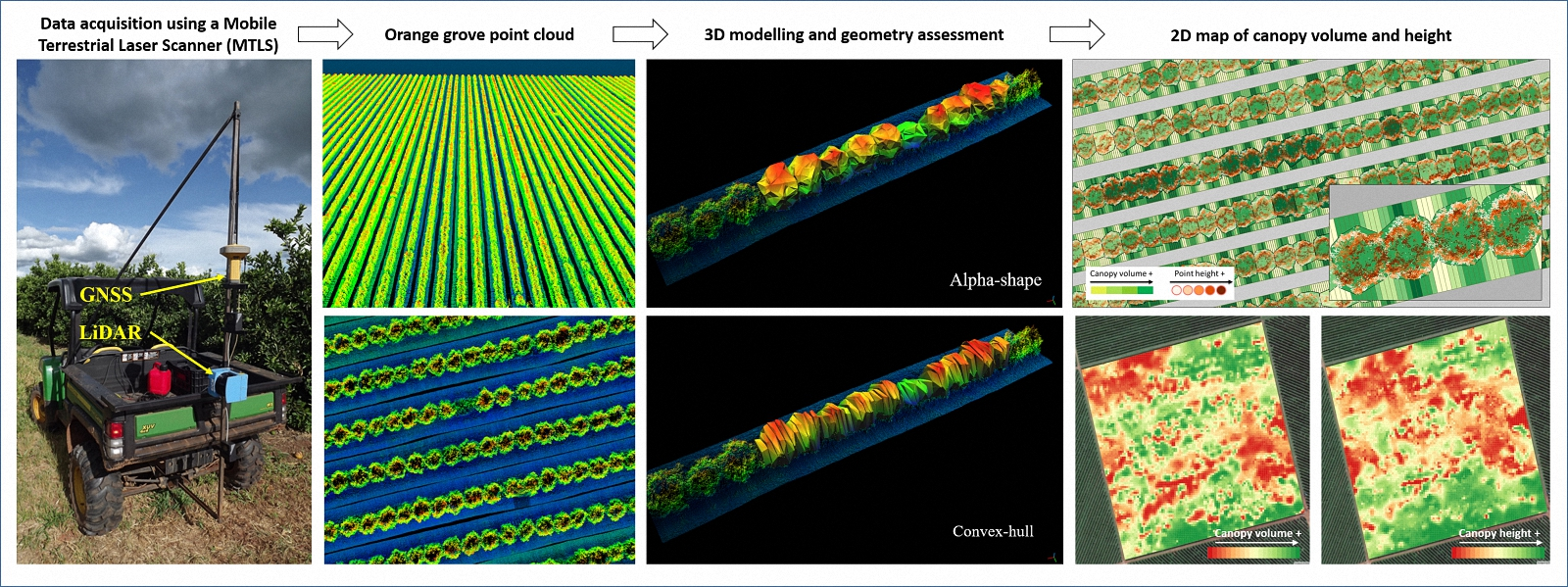
2.1. Description of Data Acquisition and Processing

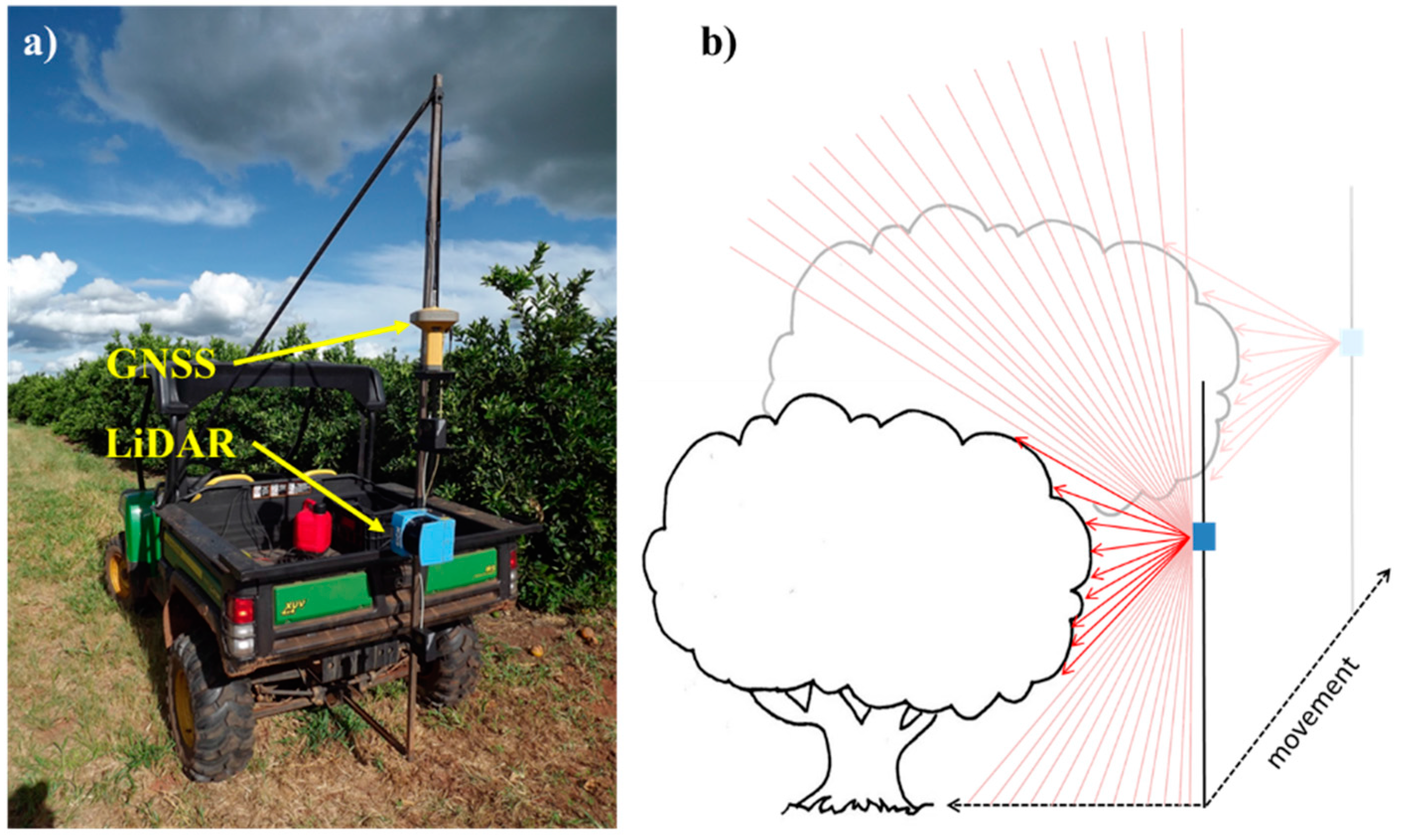
2.1.1. The Equipment and Data Acquisition

The LiDAR sensor used in this study was a terrestrial 2D laser scanner, model LMS 200 (Sick, Waldkirch, Germany). This sensor measures the distance between its center and the nearest obstacle in a given direction. The distance is estimated based on the “time-of-flight” principle. The sensor emits a laser beam which travels until it reaches the target. Then, part of the light is reflected back to the sensor. The time between the emission and reception of the laser beam is directly related to the distance between the sensor and the target.
As a 2D laser scanner, this sensor calculates distances in several directions within a plane. This is achieved through the use of an internal rotating mirror, which orientates the laser beam along the plane. For each rotation of the mirror 181 distance measurements were taken (one measurement at each degree along a 180 angle range). There were 75 rotations of the mirror per second leading to 13,575 distance measurements per second. The distance range was 8 m with 1 mm resolution.
To collect data from a commercial orange grove, the LiDAR sensor and a GR3 RTK (Real Time Kinematics) GNSS receiver (Topcon, Tokyo, Japan) with ±10 mm accuracy in kinematic mode, were arranged in a customized metallic structure mounted on an all-terrain vehicle (Figure 1a). The sensor faced the side of the tree row perpendicularly and the RTK rover unit was on top and aligned with the center of the sensor. With this setting, the sensor collected data on a 2D vertical transect along the tree row and as the vehicle moved along the alleys of the grove, the third dimension of the data was added (Figure 1b).
To acquire data from the LiDAR sensor and the RTK-GNSS receiver synchronously, a piece of software was developed using Processing (Processing v2, 2014) [22]. All communication between the computer and the LiDAR sensor was carried out by following a hexadecimal telegram code [23]. The communication with the RTK-GNSS receiver was carried out according to the NMEA (National Marine Electronics Association) standard. The maximum data acquisition frequency of the GNSS receiver was 10 Hz whereas for the LiDAR sensor was 75 Hz. The software was synchronized with the LiDAR frequency, so during the acquisition process the GNSS was linearly interpolated among the LiDAR data so that every scan had a distinct GNSS positioning. The final output from the acquisition software was a text file containing information about time, GNSS location (latitude, longitude and altitude) of the sensor and distance values for each scan.

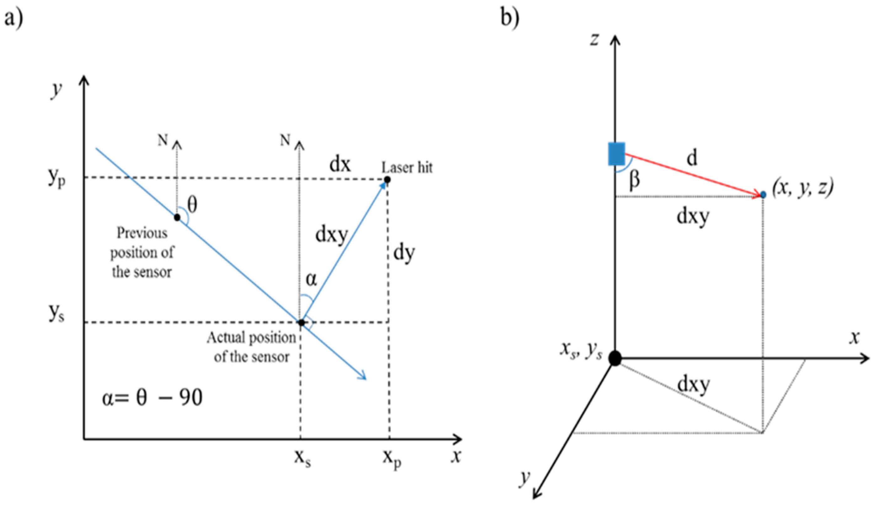
2.1.2. Data Processing

The objective of the data processing was to transform the raw data from the acquisition software into a shapefile ready to be imported into GIS software for production of thematic maps of the geometrical attributes of the trees. This goal was achieved in four steps: (i) attributing RTK-GNSS coordinates to each impact of the laser beam and generating a georeferenced 3D point cloud; (ii) filtering points of interest; (iii) classifying points into groups, each representing one individual tree or a transversal section of the tree row; and (iv) calculating the canopy volume and height of each group. The processing algorithm was developed using R software [24]. R software was chosen due to its versatility and the availability of 3D modeling tools as well as 2D spatial mapping tools. During data acquisition, the scanning of each row was saved separately so that the processing algorithm also treated each row individually.
1. Generating a georeferenced 3D point cloud
The first step consisted of transforming the raw data, which were polar coordinates (angles and distances) of the laser impacts into rectangular (Cartesian) coordinates (x, y, z) in which the x and y were UTM (Universal Transverse Mercator—Datum WGS84) coordinates derived from the RTK-GNSS receiver and z was the height of the point above the ground. Similar processing was proposed and described by Del-Moral-Martínez et al. [18].
To obtain UTM coordinates for each laser impact, the actual position of the sensor (obtained from the RTK-GNSS receiver) was shifted in the x and y axes based on the respective dx and dy deviations for each point (Equations (1) and (2)).
x p = x s + d x
y p = y s + d y
where
xp and yp are UTM coordinates of the laser impact (point) (m);
xs and ys are UTM coordinates of the sensor (m); and
dx and dy are deviations in x and y axes between the sensor and the point (m).
d x = sin α · d x y
d y = cos α · d x y
d x y = sin β · d
z p = z s ( cos β · d )
where
dxy, the distance between the sensor and the laser impact in the x, y plane (m);
α, angle of the direction of the measurement in relation to the north (degrees);
β, angle from LiDAR scanning (0 to 180°);
d, the distance value from the LiDAR scanning (m);
zp, coordinate z (height) of the point (m); and
zs, coordinate z (height) of the sensor (m).
The deviations dx and dy were calculated based on the distance between the sensor and the laser impact in the x, y plane (dxy) and the angle α (Figure 2a; Equations (3) and (4)). α corresponded to the direction of the measurement in relation to north, counted clockwise. This angle is the subtraction of 90° from the vehicle direction (θ) in relation to north (the LiDAR sensor was arranged perpendicularly to the vehicle longitude, facing the left side). The direction of the vehicle (θ) at a given moment is defined by the median values of direction from 30 consecutive points along the vehicle track, which is equivalent to a time interval of 0.5 s approximately. Finally, dxy was calculated based on the original polar coordinates of the laser impacts (distance d and angle β) (Figure 2b) (Equation (5)). The z coordinate (point height) is also derived from the polar coordinates as exposed in Equation (6). The sensor height (zs) was 1.4 m, being the reference to the point height (zp) calculation.
2. Filtering points of interest
After the transformation from polar to rectangular coordinates, the data then comprises a matrix of three columns (x, y and z) and n lines, where n is the number of laser impacts. Those data can be visualized in the form of a 3D point cloud using the CloudCompare software [25]. Figure 3 shows an example of an original point cloud from a LiDAR scanning of one crop row. A dotted line can be seen along the two sides of the tree row, which reflects the laser beam hitting the GNSS antenna. Also, whenever there is a gap between the plants the laser reached the neighbor tree row. Because the aim of the data processing was to assess canopy geometry from each tree row separately, any point that did not represent the canopy of the trees from one single row was removed from the original point cloud. For that, the next step of the processing was to apply filters to select only the points of interest (Figure 3b).
Points that were relatively far away from the target tree row were excluded by setting a maximum distance (d) for the LiDAR readings. A minimum distance value was also set to exclude obstacles that were too close to the sensor (the GNSS antenna, for example). The points which represented the soil were excluded by establishing a minimum threshold for the height (z coordinate) of each point. The output data after filtering was a point cloud representing only the crowns of the trees for a single tree row (Figure 3b).
3. Classifying points into groups
Because each file contained the 3D point cloud from one entire tree row, the point cloud had to be segmented into smaller batches prior to the computation of geometrical parameters. Two approaches were developed for this: the first divided the original point cloud from a tree row into smaller groups, each representing an individual tree; the second divided the point cloud into regular transversal sections along the row. This step allows the geometry information to be calculated for each discrete tree or for each small segment of the row.
The reason for these two different approaches is that they are applicable to two different crop scenarios. Analyzing trees individually is an appropriate approach for young crops or crops which are planted in a sparse tree spacing. Analyzing sections of the tree is applicable when the grove reaches a mature stage and the plants are large enough to fill up the gaps between them forming a continuous hedge along the row.
In order to automatically classify points among individual trees, a clustering method was applied. The cluster analysis is the grouping of similar individuals into distinct classes called clusters. In the case of this study, the mentioned “individuals” were the laser beam impacts and the “clusters” were the trees. Among the several clustering algorithms available, the chosen algorithm was k-means, which is available in R software through the “stats” package. This algorithm requires the desired number of groups to be provided prior to the classification or an initial estimation of the centers of each cluster. This estimation was based on the spacing between the trees and the length and direction of the row. The algorithm used this information as an initial guess of the cluster centers. The points were then classified (Figure 4b) according to its x and y coordinates.
The second approach for grouping the points was based on segmenting the row perpendicularly to its longitude, creating transversal sections with fixed width and length. The boundary lines of each transect were automatically drawn using the R package “sp” which allows delineation of lines and polygons using geographical information. The first step was to compute a linear regression with the x and y coordinates of the filtered point cloud, which represented the longitudinal axis of the tree row. A deviation was applied from this central line to both sides of the row forming two parallel lines containing the tree row. Finally, the row was segmented lengthwise based on a given distance (Figure 4c) and the points within each section were assigned a section identification number.
4. Calculating canopy volume and height
The actual volume of a tree canopy is strictly the volume of wood, leaves and other parts such as fruits and flowers. However, because of the limited density of points available by the scanning, the estimation of such a volume is not possible. Therefore, the canopy volume was given as the volume of a solid object that encloses the tree—this is also the concept used for canopy volume estimation in traditional field methods, as it will be further exposed. In order to compute canopy volume, a 3D object was modeled over each classified point cloud (cluster or section). Two 3D modeling algorithms available in the software R were tested in this study: the convex-hull (package “grDevices”), and the alpha-shape (package “alphashape3d”). Both algorithms were designed to produce the smallest object able to enclose a set of 3D point cloud. The first one produces a convex object and the second permits an object with concavities. The level of concavity is defined by the index α (higher α produces less concavity)—more information about the algorithms is available in Pateiro-López and Rodríguez-Casal [26] and Edelsbrunner and Mucke [27]. The canopy volume was automatically retrieved by the algorithm.
The second tree geometrical parameter, canopy height, was simply obtained by assessing the point of maximum height (z) within each group (cluster or transversal section). The final output of the processing steps was a GIS shapefile containing the polygons for each cluster or section and the canopy volume and height information.

2.2. Demonstrating and Evaluating the Proposed Method

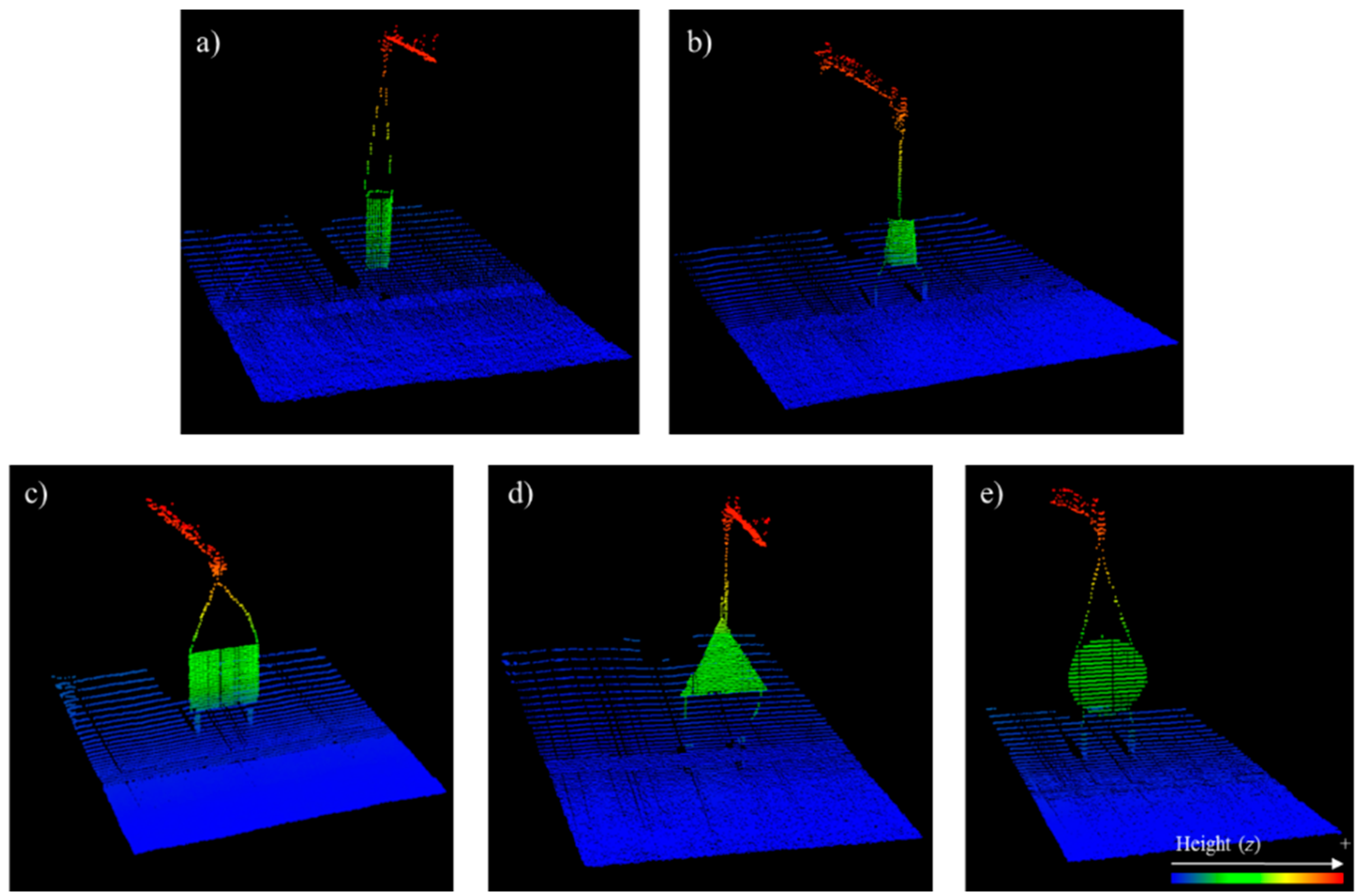
2.2.1. Validation of the Point Cloud Accuracy—Laboratory Testing

A validation focused on verifying the accuracy of the canopy volume estimation would be possible if the system was able to estimate the strict volume of above-ground parts of the canopy (wood, leaves, etc.). Measuring the actual tree volume to be taken as a reference would be laborious but not impossible—e.g., it could be achieved by using artificial trees [28] or by harvesting and immersing the tree parts into liquid [29]. However, for the present study, this cannot be used as reference for validation simply because a different type of volume is being estimated by the LiDAR system—the volume of a solid object enclosing the tree. In this case, even if several measurements of the tree boundaries were taken, it would be unlikely to provide an absolute value of volume or at least one of significant higher accuracy that could be used as a reference to the system being tested. For those reasons, the adopted validation process focused on verifying the accuracy of the point cloud as reference points of the canopy boundaries and therefore evaluate whether further canopy geometry calculations were based on reliable samples of the canopy boundary.
In order to test the overall accuracy of the point cloud produced by the system, objects with regular geometry (square, triangle, circle, cylinder, cone and body of cone) were selected as targets to be scanned. A platform carrying the sensor and the RTK-GNSS receiver was designed to run over a rail at constant speed powered by means of an electric motor. Such a testing set up was developed to minimize the effect of vibration and rotations of the sensor (rotations on its longitudinal, lateral and perpendicular, longitudinal and lateral axis—roll, pitch and yaw, respectively) during the data acquisition. A second scanning over the objects was carried out with the actual all-terrain vehicle mounting the same equipment as in the real reading in the groves. During the tests, the vehicle moved over a leveled lawn.
The accuracy of the point cloud was assessed by comparing the dimensions of the objects (side, height and diameter) in the point cloud with the actual dimensions of the objects. The dimensions from the point clouds were obtained using the CloudCompare software. The actual dimensions were obtained using a measurement tape.

2.2.2. Data Acquisition in a Commercial Orange Grove

In order to demonstrate the proposed methods for data acquisition and processing in a realistic environment, a 25 ha orange grove located in the state of São Paulo, Brazil, was scanned. The variety of the trees was “Valencia” grafted to “Swingle” rootstock. Trees were planted in 2009 and were six years old at the time of this study. The spacing was 2.6 m between trees and 6.8 m between rows. At the time of the readings, the tree canopies were already touching each other along the row, partially closing the gaps between them. The ground along the alleys were usually well leveled and there was a 12 m range of elevation over the entire area.
The developed data acquisition system and processing method were applied with the RTK-GNSS base unit mounted at the highest corner of the field. Before starting the acquisition, the RTK-GNSS base was allowed to fix its position for 30 min. The vehicle moved along the alleys at 3.3 m s−1, scanning one side of the tree row at a time. The data were saved separately for each tree row.

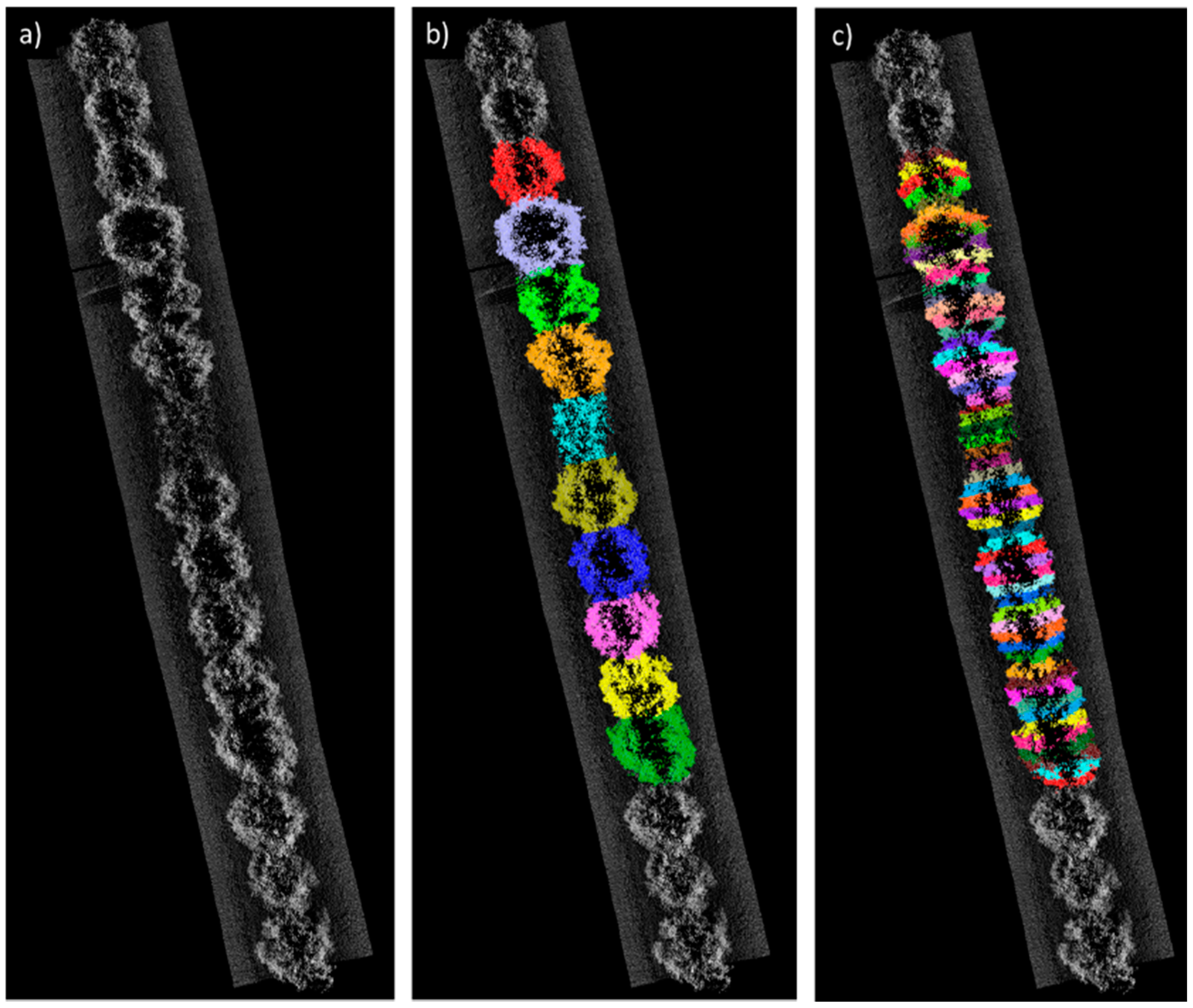
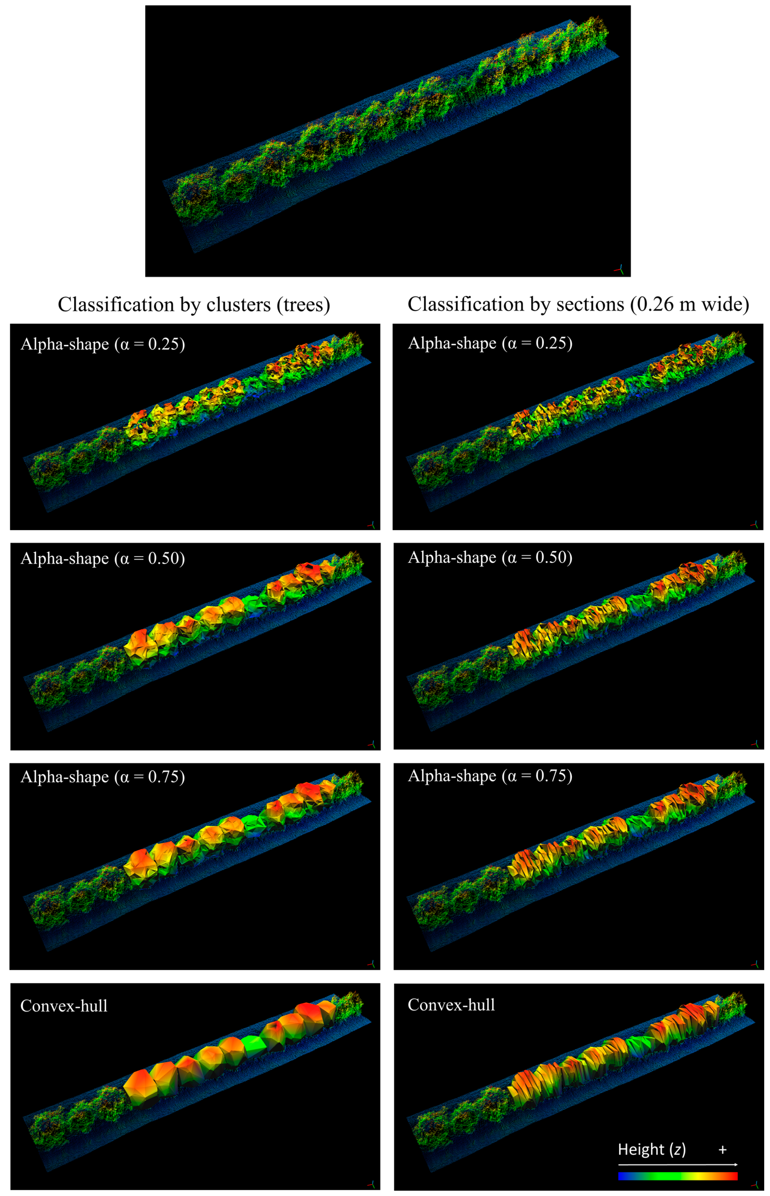
2.2.3. Evaluating Point Cloud Classification and 3D Modeling Options

As shown during the data processing description, several alternatives were used during the processing of a point cloud in order to model a 3D object over the points. To compare these possibilities, different methods were applied over a set of point clouds from 25 individual orange trees randomly selected from the scanned grove. The 3D objects were modeled over each plant individually and over transversal sections of 0.86 m, 0.52 m, 0.37 m and 0.26 m wide, which were equivalent of dividing the trees into 3, 5, 7 or 10 transversal parts, respectively. The convex-hull and the alpha-shape algorithms were applied. Variations over the alpha-shape were also tested by setting the index α to 0.25, 0.50 or 0.75. This values were considered to cover different shapes worth investigating and were arbitrarily chosen after testing a range of indexes from close to zero up to large numbers tending to infinite.
The volume of each individual tree was also computed by two additional methods based on regular geometries as are usually applied in manual methods of canopy volume estimations. In the first manual method, referred to here as “cylinder-fit”, the canopy volume is considered as two-thirds the volume of the smallest cylinder able to enclose the tree. This method was reported by Mendel [30] and Schinor et al. [31] but is not extensively adopted by growers. The second method, referred to here as “cube-fit”, is the current method adopted in most of the Brazilian groves, which is based on the tree-row-volume concept [32,33] calculated on a per-tree basis. The volume of the tree is simply given by the volume of a cube, which encloses the canopy. The dimensions of the canopy for the manual-inspired methods were measured from the point cloud of each tree using the CloudCompare software. Manual measurements were not taken due to several uncertainties related to this practice, such as the visual identification of the canopy boundaries and limitations of using standard measurement tools in a complex object such as tree canopy. In addition, this step was not meant to validate the volume estimates, but to compare the different forms of calculating volume and understand their possible differences. The proposed methods were also applied over a point cloud from a tree row segment of 10 trees for 3D visualization of the modeling and general observations.

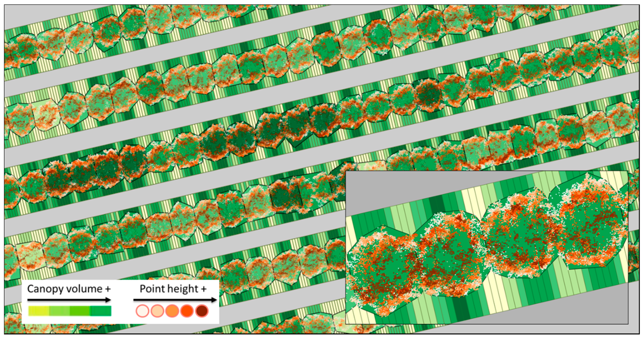
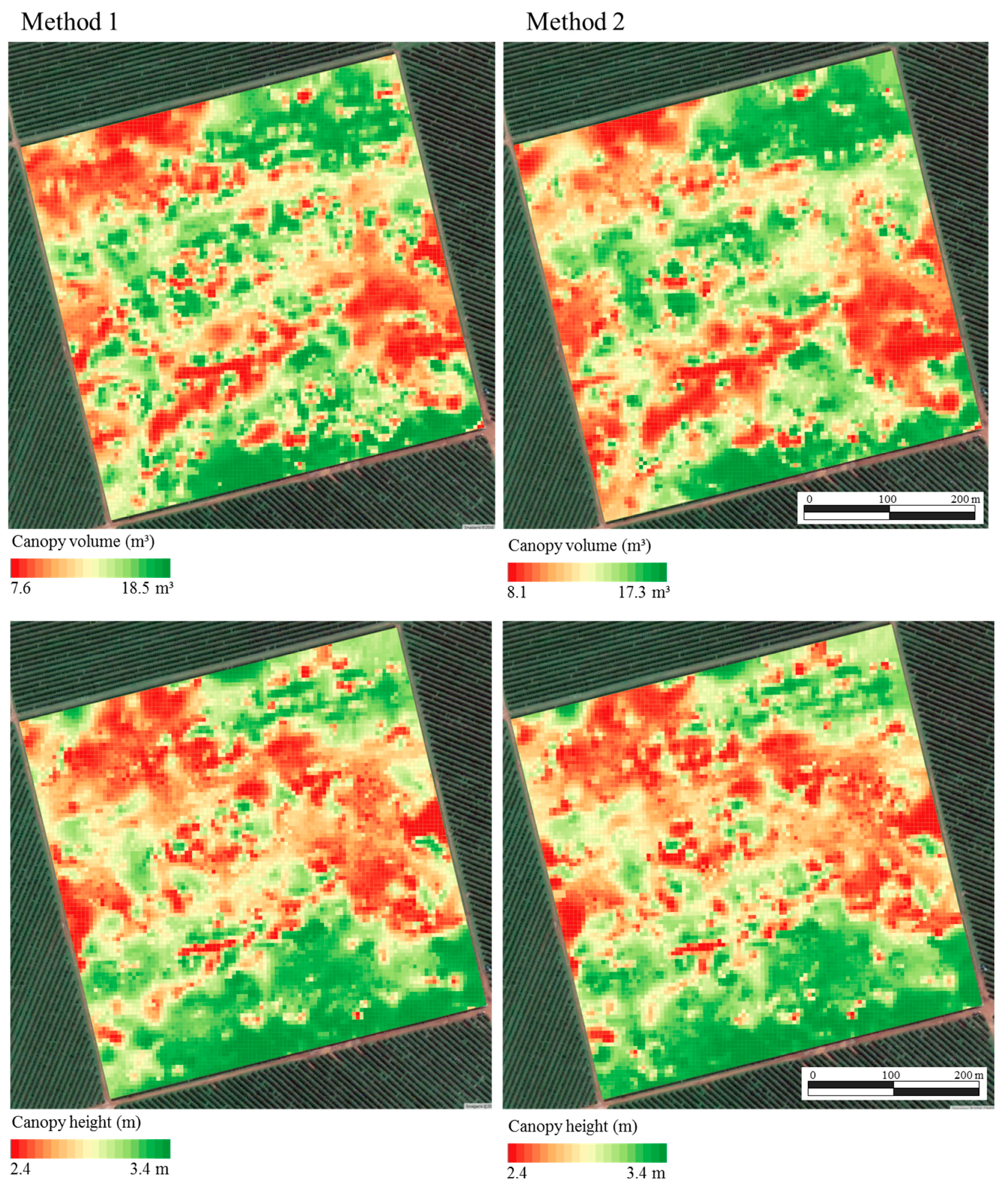
2.2.4. Mapping of Canopy Volume and Height of a Commercial Orange Grove

To produce a map of canopy volume from the scanned grove, the point cloud was processed in two different ways. The first method was based on computing the canopy volume for each individual tree (cluster) and applying the alpha-shape algorithm with the index α set to 0.75. The second approach was based on dividing the rows into sections of 0.26 m width (equivalent to dividing each tree into 10 transversal parts) and applying the convex-hull algorithm. These settings were chosen after evaluating the results from the previous analysis, which tested several options for modeling the tree canopies.
Because the trees were partially touching each other, some error in the cluster classification was expected. The accuracy of this classification was assessed by visually recognizing 678 trees from the point cloud and comparing them with the outcome of the cluster classification using the CloudCompare software.
The canopy volume and height maps were produced by importing the shapefiles from the data processing output into the QGIS software [34]. A map of points, each representing one tree or a transversal section of the row, was created by generating a centroid point within each polygon. Points within 10 m of the field boundary were excluded as well as those within a 15 m buffer around the terraces in the field. Those parts of the field were more suited to the rotation of the vehicle along its longitudinal and perpendicular axis. Because the acquisition system was neither equipped with a stabilization system nor an inertial measurement unit for further correction of sensor position deviations, the point cloud in those areas were considered more susceptible to errors and so were discarded.
Prior to map interpolation, the values from the row sections were converted into values equivalent to individual trees, otherwise the map based on sections would not be comparable with the map based on individual plants. Therefore, sections were merged in groups of 10 along the row forming segments of 2.6 m of length, which was equivalent to the tree spacing. The canopy volume of each segment was given by summing the volume of the 10 sections inside it and the height value was given by the maximum height of the 10 sections. Those parameters were attributed to a central point within each 2.6 m segment.
Finally, volume and height data at each point across the grove (representing row segments or clusters) were interpolated in a pixel grid of 5 m to produce the final canopy volume and height maps. The interpolation method was ordinary local kriging and it was carried out with the use of the Vesper 1.62 software [35].
In order to compare the resulting maps of the two methods (cluster segmentation using alpha-shape reconstruction and transversal section segmentation using convex-hull reconstruction) a similarity analysis between maps was carried out with the use of the Map Comparison Kit software [36]. The chosen algorithm was the fuzzy numerical cell-by-cell comparison. The measure of similarity (fuzzy similarity index) is given at each pixel based on Equation (7) in a scale from 0 to 1, being 1 identical values.
s ( a , b ) i = 1 | a i b i | max ( | a i | , | b i | )
where
ai, fuzzy value in pixel i from map 1;
bi, fuzzy value in pixel i from map 2; and
s(a,b)i, fuzzy similarity index in pixel i between the two maps.
The fuzzy logic implemented in this algorithm considers a level of uncertainty in the value in each pixel based on the neighboring pixels, which is referred as “fuzziness of location”. This means that the neighboring pixels affect the considered value in the central pixel. This radius of influence was set to four pixels. Other configurations for the fuzziness of location, such as the equation guiding the influence of neighboring pixels on the central pixel (a decay type function) was kept to default. More information about the algorithm is available in Hagen [37]. The relationship between maps of canopy volume and canopy height was assessed by a pixel-based correlation analysis.

3. Results and Discussion

3.1. Validation of the Point Cloud Accuracy—Laboratory Testing

The accuracy of the point cloud derived from the MTLS was assessed by using regular objects as targets for scanning. Figure 5 shows the point clouds from a range of different shaped objects scanned by the MTLS mounted on the all-terrain vehicle. These results appeared coherent based on visual assessment. The same objects were also scanned with the MTLS mounted on a platform running on a rail.
The dimensions of the objects obtained by the two scanning systems are shown in Table 1. Generally, both scanning systems provided very similar measures to the actual dimensions of the objects, with, as expected, slightly better results when the MTLS was running on the rail. The overall average error between the laser measurements and the actual dimensions of the objects was 1.4 cm (1.7%) when readings were taken using the all-terrain vehicle and 0.57 cm (0.7%) when a platform running on a rail was used, reaching a maximum difference of 5.77 cm (“b” dimension of the square with the MTLS mounted on the vehicle).
The main sources of error in such measurements are the embodied errors in the laser sensor (±5 mm) and in the RTK-GNSS (±10 mm) and the rotations of the sensor along its three axes (roll, pitch and yaw). The obtained errors in the performed tests were fairly low considering these three main sources of error. Some studies reported the importance of implementing an inertial measurement unit (IMU) during the scanning in order to register such angular displacements and correct the position of the laser impacts [10]. During the field operations, although the alleys of the groves were well leveled, higher errors might have occurred occasionally due to irregularities of the terrain.
Overall evaluation of this preliminary test indicated that the point cloud from the developed acquisition system could realistically replicate the scanned targets. In the study by Lee and Ehsani [38] the average distance error of the LMS200 sensor was 0.98 cm (aiming at a distance of 80 cm) in a static test using a wooden panel. The distance error when using orange leaves as targets was 1.17 cm. That means that, in terms of the effect of the target’s surface, the present results from tests with wooden objects can be reasonably generalized to orange tree canopies. Given the observed accuracy, further point clouds from the orange crops could be taken as reliable references for calculation of canopy geometry.

3.2. Data Acquisition in a Commercial Grove

Results from the LiDAR data acquisition and processing of a 3D point cloud over a 25 ha orange grove can be seen in Figure 6. The grove was successfully scanned as a whole. This was a particularly encouraging result since previous research which employed terrestrial laser scanners to model tree crops used smaller field plots.
The equipment setting proved to be relatively robust for large field scanning. One issue that should be reported is the sensitivity of the LiDAR sensor to intense sunlight exposure. The sensor used in this study was developed for indoor scanning and does not operate properly under excessive light exposure. Several times during the data acquisition in the field, the operation was interrupted due to malfunctioning of the sensor. Sensors developed for outdoor purposes are available on the market and would be more appropriate for agricultural use. Otherwise, a structure to protect the sensor against direct sunlight without blocking its field of vision towards the targets should be required. Avoiding readings during hours of intense light exposure is also an option to deal with this issue.
It is noticeable that the achieved density of points was able to capture the shape of the rows and of individual trees with good level of detail. With the applied data acquisition configuration (75 Hz scanning frequency at 3.3 m s−1 speed) the distance between each scan was around 4 cm. The total grove accounted for approximately 175 million points, which corresponds to approximately 700 points m−2 (approximately 12,100 points per plant). Airborne LiDAR scanning applied over urban or forest areas usually produces point clouds with 0.5 to 5 points m−2. Escolà et al. [7] reported a density of 8000 points per m−2 using a multi-echo LiDAR device on a MTLS on an olive grove but they were using a sensor with higher angular resolution traveling at a slower forward speed.
The forward speed used for scanning is compatible with several mechanical operations in the grove such as spraying, which means that the LiDAR-based system could be attached to the machines in the field to collect data while performing other agricultural operations.

3.3. Modeling of 3D Objects from the Point Cloud

The results from the proposed 3D modeling algorithms applied to a segment of 10 trees are shown in Figure 7. One premise that can be used to evaluate the outcome from the different algorithms is the amount of points at the canopy boundary being used to create the 3D object representing the tree. The higher the number of points the closer the estimation gets to the actual tree volume. It is noticeable how the convex-hull model apparently used less points to generate the 3D model resulting in larger objects since salient branches enlarge the hull structure. As expected, the external profile of the canopy was better represented by the alpha-shape algorithm with lower α index. However, the index α should be appropriately set. A low index might produce disconnected structures forming holes inside the canopy, which is not desirable for the adopted approach of canopy volume. Because this algorithm permits the representation of concave structures, it is reasonable to consider the alpha-shape as a suitable model for representing the tree canopy. Likewise, it is noticeable that slicing the row into transversal sections instead of maintaining the tree as a whole also helped the representation of the canopies with greater level of detail. The segmentation of the trees was particularly important in the convex-hull model, because it reduced the effect of over estimation caused by outer branches on the tree by using a greater amount of points to generate the 3D model of each plant. This issue was more severe when the model was created over the entire plant. The importance of segmenting the point cloud when applying the convex-hull algorithm to estimate volume was also evidenced by Auat Cheein et al. [19].
However, when slicing the trees to produce 3D models of continuous canopies a problem with the alpha-shape algorithm arose. While the algorithm produced desirable concavities on the outer part of the canopy, which helped in detailing its silhouette, it also created undesirable depressions in the transversal slicing plane and at the bottom of the trees (Figure 8). When all the sections were put together, the concavities in the transversal wall of the sections produced voids, which affected the final canopy volume computation. The voids between sections were also present in the convex-hull models but they were considered insignificant (Figure 9). They are inherent to the approach of slicing the rows and are directly related to the scanning frequency during the data acquisition (which determines the spacing between scans). Because of the high scanning frequency, the space between each scan was very narrow and so were the voids between the convex-hull objects (Figure 9). Thus, the convex-hull algorithm was considered a better option than the alpha-shape to represent transversal sections of the row. On the other hand, the alpha-shape algorithm remained a better option when the model was applied over the entire tree. As a guideline to choose the α index, the best α should be the one which produces the smallest volume—or that uses that highest amount of reference points—whilst maintaining the canopy as a solid object (without voids). Amongst the tested options, this result was obtained when α was set to 0.75 (Figure 10), through simple visual assessment. In order to determine the optimum α a thorough investigation is still needed, testing more α options and with more robust evaluation techniques.
The results from the measurements of 25 individual trees extracted from the scanned grove indicate that combining different options of 3D modeling and segmentation can result in significantly different canopy volume estimations (Table 2). As noticed in previous observations, the convex-hull model resulted in the highest canopy volume, followed by the alpha-shape with higher α. The canopy volume decreased as the number of slices increased, resulting in significantly different volumes, especially for the α-shape algorithms. The differences between algorithms were even more evident as the number of slices increased (notice that in lower number of sections the alpha set to 0.75 or 0.5 yielded similar results and when the number of sections increased all algorithms resulted in significantly different outcomes). When compared with the convex-hull, the higher decrease in the alpha-shape algorithms when increasing the number of sections per tree was probably due to the increase in voids between sections as mentioned. A twofold-range in volume was noticed in alpha-shape algorithms when the trees were taken as a whole or divided into 10 sections.
It should be noted that the rough simplification of the canopy structure by the method based on the cube-fit, the common practice used in Brazil, overestimated the canopy volume in relation to all the other algorithms. The cylinder-fit, which applied a correction of two third off the whole object, got similar results to the α-shape with alpha set to 0.5. As shown previously (Figure 10), even being able to realistically represent the canopy, this algorithm can produce voids inside the plant, which is not desirable for canopy volume estimation.
The average volume obtained from the alpha-shape with index of 0.75, which was previously considered an adequate representation of individual trees, was 14.3 m3 per plant using an average of approximately 6600 points as references for measurements, whereas the convex-hull, considered a good option when trees were divided into sections, resulted in an average canopy volume of 12.8 m3 using approximately 3400 points in 10 sections. Canopy volumes from manual measurements based on the cube-fit and the cylinder-fit were 22.6 m3 and 11.9 m3, respectively (Table 2), using a significantly reduced amount of reference points. The difference in canopy volume obtained from the different methods is evidence of the importance of the adoption of a reference method. At this stage, it is reasonable to consider that the method of canopy volume computation based on the MTLS and 3D modeling is clearly more capable of capturing the geometry of the canopy than the current available manual methods based on regular geometries such as cubes or cylinders because it employs a remarkably greater number of reference points for measurements. Thorough investigation over the algorithms is still needed before changing to a new standardized system. Nevertheless, the LiDAR-based methods are applicable in the field and should be considered as a possible standard for canopy volume computation.
Regardless of the specific algorithm choice for standardization, any new system to be adopted for the grove management would require a new set of calibrations based on empirical experimentation in order to transform canopy volume readings into actual input rates for spraying, fertilizer application, irrigation, etc. The level of canopy detail provided by the system, even if not entirely true to the real canopy volume, would necessarily have to be worth in terms of the actually enhancing input recommendations.
For the purposes of this study, these first considerations of 3D modeling methods indicate that, among the tested options, the best algorithm for modeling the canopy of individual trees was the alpha-shape with index α set to 0.75, because it permitted the representation of salient structures from the canopy whilst keeping the canopy as a solid without voids inside it. The convex-hull algorithm was a better option for modeling sections of the trees, because it produced minimum voids between them. The weakness of this algorithm, which is overestimating the structure in outer parts of the tree, is less relevant when the tree is divided into sections. For those reasons, these two approaches were chosen to be further applied on this study.

3.4. Mapping of Canopy Volume and Height in a Commercial Orange Grove

The final canopy volume and height maps were produced by two methods: (Method 1) by classifying the point cloud into individual trees (cluster) and subsequently applying the alpha-shape algorithm (α = 0.75); and (Method 2) by dividing the rows into 0.26 m long sections and subsequently applying the convex-hull algorithm to model the canopies. The two data processing methods produced polygon shapefiles where each polygon contained the information of canopy volume and height computed by the algorithms (Figure 11). The slicing of the rows produced approximately 10 polygons per tree (prior to interpolation every 10 subsequent section were merged together to produce the final map). Inside each polygon, approximately 6 laser scans were found. In the representation of individual trees, the cluster classification accuracy was 90.2% (percent of correctly classified clusters over the total number of clusters). This was considered sufficient to produce reliable information maps, but this accuracy may vary from different groves.
The two chosen methods produced similar canopy volume and height maps. The final maps were visually similar (Figure 12) and had similar basic statistical parameters (Table 3). It should be expected that if the trees in one grove form a continuous hedge along the row, the section approach would be ideal, whereas if the trees are discrete, the cluster classification would be the best option. In the evaluated grove, it seems likely that at the particular development stage of this grove, either method was appropriate for mapping without major consequences for the form of the final maps. One thing to be noticed is that the average canopy volume and height estimated from the maps were quite similar between the methods (11.94 m3 and 12.13 m3 for Methods 1 and 2, respectively—Table 3), which was not the case when 25 trees were analyzed separately (14.1 and 12.8 m3 for Methods 1 and 2, respectively—Table 2). It should also be noted that, when analyzing results from the entire grove, a range of different targets (gaps, trees with different size, shape and density, etc.) are being scanned which was not the case for the selected 25 trees. The different algorithms and classifications options might perform differently depending on the target characteristics, and, for that reason, further investigations are needed in order to better understand what aspects can affect the results.
The similarity between the maps, as assessed by the fuzzy similarity index, was higher for the canopy height (fuzzy similarity index = 0.99) than for the canopy volume. This is probably because both methods applied the same rationale to compute the height. The canopy volume maps were computed by two different algorithms (which were more complex than taking the highest point for height computation), so the fuzzy comparison resulted in a slightly lower index (fuzzy similarity index = 0.96).
Some correlation between height and canopy volume was also expected. This was higher when the two parameters were computed using the cluster analysis (r = 0.71). The grouping of sections along the row did not necessarily match with individual plants, so the correlation of height and volume was not as high (r = 0.61).
Generally, both methods performed similarly. They were both able to represent the spatial variability of canopy geometry in the grove. These maps are a useful basis for site-specific management, such as variable rate spraying and for dividing the field into management zones.

4. Conclusions

A methodology for 3D modeling and canopy geometry computation for orange groves was developed using a mobile terrestrial laser scanning system based on a LiDAR sensor. The data acquisition and processing systems were described and variations over the 3D modeling algorithms were demonstrated and compared.
The method for data acquisition and processing proved to produce reliable georeferenced point clouds of a commercial orange grove. The data acquisition set up was robust for large field scanning and could be implemented on current agricultural operations in the groves.
The convex-hull and alpha-shape (α = 0.75) 3D modeling algorithms worked best when implemented over transversal sections of the row and over individualized plants, respectively. Varying the type of segmentation of the point cloud and the 3D modeling algorithms resulted in different values of canopy volume indicating the need for a reference method to be adopted. Nevertheless, the mapping of canopy volume and height by either cluster or section of the row resulted in similar spatial variability.
The proposed data acquisition and processing systems were able to produce useful information for precision agriculture management. The LiDAR-based scanning and the proposed data processing and mapping reproduced the spatial variability in the grove in the format of thematic maps that can be used for variable rate applications and to guide management zones delineations within the grove. All the software used is open-source and freely available to any user.

Acknowledgments

We thank Citrosuco and Jacto companies for supporting this project, the São Paulo Research Foundation (FAPESP) for providing a scholarship to the first author (grant: 2013/18853-0) and the Coordination for the Improvement of Higher Education Personnel (CAPES), for funding the first author as an exchange visitor at the University of Lleida (grant: bex_3751/15-5). We also like to thank Rob Bramley for general comments and English language editing.

Author Contributions

André F. Colaço conceived the study, participated in the development of the data acquisition and processing systems, collected the field data, interpreted the results and wrote the manuscript. Rodrigo G. Trevisan did the main development and programing of the data acquisition and processing software and contributed to field data acquisition. José P. Molin contributed to the conception, development and coordination of the project and helped in the interpretation of the results. Joan R. Rosell-Polo and Alexandre Escolà contributed to the data analysis and interpretation. All authors contributed to the edition of the manuscript.

Conflicts of Interest

The authors declare no conflict of interest.

References

  1. Dworak, V.; Selbeck, J.; Ehlert, D. Ranging sensors for vehicle-based measurement of crop stand and orchard parameters: A review. Trans. ASABE 2011, 54, 1497–1510. [Google Scholar] [CrossRef]
  2. Rosell-Polo, J.R.; Sanz, R. A review of methods and applications of the geometric characterization of tree crops in agricultural activities. Comput. Electron. Agric. 2012, 81, 124–141. [Google Scholar] [CrossRef]
  3. Berk, P.; Hocevar, M.; belsak, A. Development of alternative plant protection product application techniques in orchards, based on measurement sensing systems: A review. Comput. Electron. Agric. 2016, 124, 273–288. [Google Scholar] [CrossRef]
  4. Gil, E.; Arnó, J.; Llorens, J.; Sanz, R.; Llop, J.; Rosell-Polo, J.R.; Gallart, M.; Escolà, A. Advanced technologies for the improvement of spray application techniques in Spanish viticulture: An overview. Sensors 2014, 14, 691–708. [Google Scholar] [CrossRef] [PubMed] [Green Version]
  5. Underwood, J.P.; Hung, C.; Whelan, B.; Sukkarieh, S. Mapping almond orchard canopy volume, flowers, fruit and yield using lidar and vision sensors. Comput. Electron. Agric. 2016, 130, 83–96. [Google Scholar] [CrossRef]
  6. Underwood, J.P.; Jagbrant, G.; Nieto, J.I.; Sukkarieh, S. Lidar-Based Tree Recognition and Platform Localization in Orchards. J. Field Robot. 2015, 32, 1056–1074. [Google Scholar] [CrossRef]
  7. Escolà, A.; Martínez-Casasnovas, J.A.; Rufat, J.; Arnó, J.; Arbonés, A.; Sebé, F.; Pascual, M.; Gregorio, E.; Rosell-Polo, J.R. Mobile terrestrial laser scanner applications in precision fruticulture/horticulture and tools to extract information from canopy point clouds. Precis. Agric. 2017, 18, 111–132. [Google Scholar] [CrossRef]
  8. Escolà, A.; Rosell-Polo, J.R.; Planas, S.; Gil, E.; Pomar, J.; Camp, F.; Llorens, J.; Solanelles, F. Variable rate sprayer. Part 1—Orchard prototype: Design, implementation and validation. Comput. Electron. Agric. 2013, 95, 122–135. [Google Scholar] [CrossRef]
  9. Chen, Y.; Zhu, H.; Ozkan, H.E. Development of a variable-rate sprayer with laser scanning sensor to synchronize spray outputs to tree structures. Trans. ASABE 2012, 55, 773–781. [Google Scholar] [CrossRef]
  10. Rosell-Polo, J.R.; Gregorio, E.; Gené, J.; Llorens, J.; Torrent, X.; Arnó, J.; Escolà, A. Kinect v2 sensor-based mobile terrestrial laser scanner for agricultural outdoor applications. IEEE/ASME Trans. Mech. 2017. [Google Scholar] [CrossRef]
  11. Méndez, V.; Rosell-Polo, J.R.; Sanz, R.; Escolà, A.; Catalán, H. Deciduous tree reconstruction algorithm based on cylinder fitting from mobile terrestrial laser scanned point clouds. Biosyst. Eng. 2014, 124, 78–88. [Google Scholar] [CrossRef]
  12. Del-Moral-Martínez, I.; Rosell-Polo, J.R.; Company, J.; Sanz, R.; Escolà, A.; Masip, J.; Martínez-Casasnovas, J.A.; Arnó, J. Mapping vineyard leaf area using mobile terrestrial laser scanners: should rows be scanned on-the-go or discontinuously sampled? Sensors 2016, 16, 119. [Google Scholar] [CrossRef] [PubMed]
  13. Arnó, J.; Escolà, A.; Rosell-Polo, J.R. Setting the optimal length to be scanned in rows of vines by using mobile terrestrial laser scanners. Precis. Agric. 2017, 18, 145–151. [Google Scholar] [CrossRef]
  14. Lee, K.H.; Ehsani, R. A laser scanner based measurement system for quantification of citrus tree geometric. Appl. Eng. Agric. 2009, 25, 777–788. [Google Scholar] [CrossRef]
  15. Rosell-Polo, J.R.; Llorens, J.; Sanz, R.; Arnó, J.; Ribes-Dasi, M.; Masip, J.; Escolà, A.; Camp, F.; Solanelles, F.; Gràcia, F.; et al. Obtaining the three-dimensional structure of tree orchards from remote 2D terrestrial LIDAR scanning. Agric. For. Meteorol. 2009, 149, 1505–1515. [Google Scholar] [CrossRef]
  16. Tumbo, S.D.; Salyani, M.; Whitney, J.D.; Wheaton, T.A.; Miller, W.M. Investigation of laser and ultrasonic ranging sensors for measurements of citrus canopy volume. Appl. Eng. Agric. 2002, 18, 367–372. [Google Scholar] [CrossRef]
  17. Wei, J.; Salyani, M. Development of a laser scanner for measuring tree canopy characteristics: Phase 1. Prototype development. Trans. ASABE 2004, 47, 2101–2108. [Google Scholar] [CrossRef]
  18. Del-Moral-Martínez, I.; Arnó, J.; Escolà, A.; Sanz, R.; Masip-Vilalta, J.; Company-Messa, J.; Rosell-Polo, J.R. Georeferenced Scanning System to Estimate the LeafWall Area in Tree Crops. Sensors 2015, 15, 8382–8405. [Google Scholar] [CrossRef] [PubMed]
  19. Auat Cheein, F.A.; Guivant, J.; Sanz, R.; Escolà, A.; Yandún, F.; Torres-Torriti, M.; Rosell-Polo, J.R. Real-time approaches for characterization of fully and partially scanned canopies in groves. Comput. Electron. Agric. 2015, 118, 361–371. [Google Scholar] [CrossRef]
  20. Food and Agriculture Organization (FAO). Faostat. 2014. Available online: http://faostat.fao.org (accessed on 2 April 2017).
  21. Colaço, A.F.; Molin, J.P. Variable rate fertilization in citrus: A long term study. Precis. Agric. 2017, 18, 169–191. [Google Scholar] [CrossRef]
  22. Processing v2, 2014. Available online: https://processing.org (accessed on 28 October 2014).
  23. SICK AG. Telegrams for Operating/Configuring the LMS2XX Laser Measurement Systems; Firmware Version V.2.10/X1.14; 2003. Available online: http://sicktoolbox.sourceforge.net/docs/sick-lms-telegram-listing.pdf (accessed on 28 October 2014).
  24. R v3.2.2—R Core Team. R: A Language and Environment for Statistical Computing; Software; R Foundation for Statistical Computing: Vienna, Austria, 2015; Available online: http://www.R-project.org (accessed on 13 May 2015).
  25. CloudCompare [GPL Software] v2.6.1. 2015. Available online: http://www.cloudcompare.org (accessed on 15 March 2015).
  26. Pateiro-López, B.; Rodríguez-Casal, A. Generalizing the convex-hull of a sample: The R package alphahull. J. Stat. Softw. 2010, 34. [Google Scholar] [CrossRef]
  27. Edelsbrunner, H.; Mucke, E.P. Three-Dimensional alpha shapes. ACM Trans. Graph. 1994, 13, 43–72. [Google Scholar] [CrossRef]
  28. Van der Zande, D.; Hoet, W.; Jonckheere, I.; van Aardt, J.; Coppin, P. Influence of measurement set-up of ground-based LiDAR for derivation of tree structure. Agric. For. Meteorol. 2006, 141, 147–160. [Google Scholar] [CrossRef]
  29. Velázquez-Martí, B.; Estornell, J.; López-Cortéz, I.; Martí-Gavilá, J. Calculation of biomass volume of citrus trees from an adapted dendrometry. Biosyst. Eng. 2012, 112, 285–292. [Google Scholar] [CrossRef]
  30. Mendel, K. Rootstock-scion relationships in Shamouti trees on light soil. Katavim 1956, 6, 35–60. [Google Scholar]
  31. Schinor, E.H.; Cristofani-Yaly, M.; Bastianel, M.; Machado, M.A. Sunki Mandarin vs Poncirus trifoliate hybrids as rootstocks for Pera sweet orange. J. Agric. Sci. 2013, 5, 190–200. [Google Scholar] [CrossRef]
  32. Scapin, M.S.; Behlau, F.; Scandelai, L.J.M.; Fernandes, R.S.; Silva, G.J., Jr.; Ramos, H.H. Tree-row-volume-based sprays of copper bactericide for control of citrus canker. Crop Prot. 2015, 77, 119–126. [Google Scholar] [CrossRef]
  33. Silva, G.J., Jr.; Scapin, M.S.; Silva, F.P.; Silva, A.R.P.; Behlau, F.; Ramos, H.H. Spray volume and fungicide rates for citrus black spot control based on tree canopy volume. Crop Prot. 2016, 85, 38–45. [Google Scholar] [CrossRef]
  34. QGIS v2.10—QGIS Development Team. QGIS Geographic Information System. Open Source Geospatial Foundation Project. 2015. Available online: http://www.qgis.org (accessed on 15 March 2015).
  35. Minasny, B.; McBratney, A.B.; Whelan, B.M. VESPER Version 1.62; Precision Agriculture Laboratory, Faculty of Agriculture and Environment, University of Sydney: Sydney, Australia, 2006. [Google Scholar]
  36. Map Comparison Kit v3.2. 2016. Available online: http://mck.riks.nl (accessed on 17 December 2016).
  37. Hagen, A. Fuzzy set approach to assessing similarity of categorical maps. Int. J. Geogr. Inf. Sci. 2003, 17, 235–249. [Google Scholar] [CrossRef]
  38. Lee, W.S.; Ehsani, R. Comparison of two 2D laser scanners for sensing object distances, shapes, and surfaces patterns. Comput. Electron. Agric. 2008, 60, 250–262. [Google Scholar] [CrossRef]
Figure 1. (a) LiDAR (Light Detection and Ranging) sensor and GNSS (Global Navigation Satellite System) receiver mounted on an all-terrain vehicle; and (b) diagram of LiDAR sensor 2D scanning and displacement along the alleys.
Remotesensing 09 00763 g001
Figure 2. (a) dx and dy deviations based on the angle α and dxy; and (b) dxy based on distance d and angle β.
Remotesensing 09 00763 g002
Figure 3. (a) Original point cloud from one tree row; and (b) point cloud after the filtering process.
Remotesensing 09 00763 g003
Figure 4. (a) Top view of a non-classified point cloud from orange trees; (b) clustering classification into groups each representing an individual tree; and (c) classification of points in transversal sections along the row.
Remotesensing 09 00763 g004
Figure 5. Point clouds from objects scanned with a mobile terrestrial laser scanner mounted on an all-terrain vehicle: (a) cylinder; (b) body of cone; (c) square; (d) triangle; and (e) circle.
Remotesensing 09 00763 g005
Figure 6. 3D georeferenced point cloud derived from the developed mobile terrestrial laser scanning system used in a 25 ha commercial orange grove.
Remotesensing 09 00763 g006
Figure 7. Convex-hull and alpha-shape algorithms to model orange trees according to two approaches: clusters (individual trees) and transversal sections of the row (0.26 m long). The top picture is an image of the point cloud.
Remotesensing 09 00763 g007
Figure 8. Detail of the convex-hull and alpha-shape models over a single 0.26 m long transversal section of a tree row.
Remotesensing 09 00763 g008
Figure 9. Top view of the convex-hull modeling over transversal sections of an orange tree row.
Remotesensing 09 00763 g009
Figure 10. 3D canopy structure of a single tree modeled according to different algorithms. The top picture is an image of the point cloud.
Remotesensing 09 00763 g010
Figure 11. Shapefiles produced after either segmenting the row into transversal sections or into individual trees.
Remotesensing 09 00763 g011
Figure 12. Canopy volume and height maps generated according to the two data processing methods: Method 1, classifying the point cloud into individual trees (cluster) and subsequently applying the alpha-shape algorithm (α = 0.75); and Method 2, dividing the rows into 0.26 m long sections and further applying the convex-hull algorithm.
Remotesensing 09 00763 g012
Table 1. Object dimensions measured manually and by a mobile terrestrial laser scanner mounted on an all-terrain vehicle and on a platform running over a rail.
Objectsabc
(i)(ii)(iii)(i)(ii)(iii)(i)(ii)(iii)
(cm)
Square98.6098.29100.0094.23100.25100.00---
Triangle98.2298.33100.0084.6488.4887.00---
Circle101.1799.96100.00------
Cylinder I79.5879.7880.0029.5830.1330.00---
Cylinder II80.9283.2183.0019.7420.2820.00---
Body of cone62.6563.3164.0044.9545.0545.0031.1530.9031.00
Header abbreviations: (i) laser scanner mounted on an all-terrain vehicle; (ii) laser scanner mounted on a platform running on a rail; and (iii) actual dimension (by measurement tape).Remotesensing 09 00763 i001
Table 2. Mean canopy volume of 25 individual trees estimated by different methods and by dividing the trees into different number of sections.
AlgorithmNumber of Sections Per Tree
135710
Mean Canopy Volume of 25 Individual Trees (m3)
Cube-fit22.65a----
Cylinder-fit11.90c----
Convex-hull16.07b,a14.71a,ab13.97a,ab13.46a,ab12.86a,b
α-shape (α = 0.75)14.31c,a11.57b,b10.02b,bc8.66b,cd7.34b,d
α-shape (α = 0.50)12.16c,a9.77b,b8.19b,bc6.98c,cd5.72c,d
α-shape (α = 0.25)6.19d,a5.32c,b4.47c,bc4.15d,c3.34d,d
Letters before and after comma mean values are different within column and line, respectively (at 5% significance).
Table 3. Descriptive statistics of canopy volume and height maps for the two proposed methods.
Canopy VariableMethod *MeanMinimumMaximumCoef. of Variation
m3
Volume111.947.6418.570.09
212.138.0517.300.09
m
Height12.852.473.390.03
22.872.443.430.04
* Method 1: classifying the point cloud into individual trees (cluster) and subsequently applying the alpha-shape algorithm (α = 0.75). Method 2: dividing the rows into 0.26 m long sections and further applying the convex-hull algorithm.

