Correcting InSAR Topographically Correlated Tropospheric Delays Using a Power Law Model Based on ERA-Interim Reanalysis


1
SAR/InSAR Engineering Applications Laboratory (SEAL), Nanjing Institute of Surveying, Mapping & Geotechnical Investigation, Co., Ltd., Nanjing 210019, China
2
School of Geodesy and Geomatics, Wuhan University, Wuhan 430079, China
3
College of Geoscience and Surveying Engineering, China University of Mining & Technology, Beijing 100083, China
*
Author to whom correspondence should be addressed.
Remote Sens. 2017, 9(8), 765; https://doi.org/10.3390/rs9080765
Submission received: 20 June 2017
/
Revised: 20 July 2017
/
Accepted: 20 July 2017
/
Published: 26 July 2017
(This article belongs to the Section Atmospheric Remote Sensing)
Abstract
:Tropospheric delay caused by spatiotemporal variations in pressure, temperature, and humidity in the lower troposphere remains one of the major challenges in Interferometric Synthetic Aperture Radar (InSAR) deformation monitoring applications. Acquiring an acceptable level of accuracy (millimeter-level) for small amplitude surface displacement is difficult without proper delay estimation. Tropospheric delay can be estimated from the InSAR phase itself using the spatiotemporal relationship between the phase and topography, but separating the deformation signal from the tropospheric delay is difficult when the deformation is topographically related. Approaches using external data such as ground GPS networks, space-borne spectrometers, and meteorological observations have been exploited with mixed success in the past. These methods are plagued, however, by low spatiotemporal resolution, unfavorable weather conditions or limited coverage. A phase-based power law method recently proposed by Bekaert et al. estimates the tropospheric delay by assuming the phase and topography following a power law relationship. This method can account for the spatial variation of the atmospheric properties and can be applied to interferograms containing topographically correlated deformation. However, the parameter estimates of this method are characterized by two limitations: one is that the power law coefficients are estimated using the sounding data, which are not always available in a study region; the other is that the scaled factor between band-filtered topography and phase is inverted by least squares regression, which is not outlier-resistant. To address these problems, we develop and test a power law model based on ERA-Interim (PLE). Our version estimates the power law coefficients by using ERA-Interim (ERA-I) reanalysis. A robust estimation technique was introduced in the PLE method to estimate the scaled factor, which is insensitive to outliers. We applied the PLE method to ENVISAT ASAR images collected over Southern California, US, and Tianshan, China. We compared tropospheric corrections estimated from using our PLE method with the corrections estimated using the linear method and ERA-I method. Accuracy was evaluated by using delay measurements from the Medium Resolution Imaging Spectrometer (MERIS) onboard the ENVISAT satellite. The PLE method consistently delivered greater standard deviation (STD) reduction after tropospheric corrections than both the linear method and ERA-I method and agreed well with the MERIS measurements.
1. Introduction
Interferometric synthetic aperture radar (InSAR) is a global all-weather remote sensing technique that can generate a high-precision surface deformation map with a high spatial resolution for large areas. Typically, a standard frame of ENVISAT ASAR in strip map mode covers approximately 100 km2 with 30 m resolution. Atmospheric delay error, however, poses one of the major challenges to InSAR geodesy, especially for monitoring deformation signals with small magnitude and long wavelength. These deformation signals could be due to regional surface subsidence [1], landslides [2], volcanic eruptions [3], tidal loading [4], tectonic slow slip [5], and earthquakes [6]. Atmospheric delays are typically introduced by the ionosphere and the troposphere when radio signals propagate through the atmosphere. Although the observed atmospheric delay in InSAR is due to these two terms, the major challenge mainly comes from tropospheric delay because of its high spatiotemporal variability. Spatiotemporal variations in the free electrons of the ionosphere (60 km) cause phase advances of the radio signals that are only significant at higher latitudes and for larger wavelength radar signals, such as the L and P bands [7]. Tropospheric effects are due to variations in pressure, temperature, and relative humidity in the lower part of the troposphere (12 km) that often lead to phase delays up to a few decimeters in magnitude and overwhelm the deformation signal of interest [8,9]. This study focuses on estimating topographically correlated tropospheric delay. We were not concerned with ionospheric effects because we used only C-band SAR images in our test.
Many methods have been developed to estimate the tropospheric delay on InSAR [10,11,12]. In general, the approaches for mitigating tropospheric delay can be classified into two categories: those using ancillary delay measurements and empirical models based on the interferometric phase itself.
The methods based on ancillary datasets produce synthetic delay maps directly by external sources such as GPS wet delay measurements [13,14,15], multispectral imagery such as Moderate Resolution Imaging Spectroradiometer (MODIS) and Medium Resolution Imaging Spectrometer (MERIS) [16,17], GPS integrated with spectrometer data [18], and local or global meteorological reanalysis products [19,20,21]. The advantages of these methods are their straightforwardness and the fact that they do not need a priori information about surface deformation and assumptions regarding the temporal correlation of the troposphere. However, methods using ancillary delay measurements are limited by the spatiotemporal resolution and coverage of the data source. Furthermore, weather conditions and sunlight dependency may reduce the quality of the multispectral imagery available for the study region. Following recent advances in the global atmospheric model (GAM), atmospheric models are now regarded as the most promising method of tropospheric correction for InSAR [22,23,24,25,26]. GAM provides atmospheric parameters (pressure, temperature, and humidity) that can be applied to calculate the refractivity equations and determine path delays. The distinctive features of GAMs include their availability under all weather conditions regardless of cloud presence and relatively high spatial resolution. The ERA-Interim (ERA-I) has a resolution of ~75 km [27] and the Weather Research and Forecasting (WRF) model has a resolution of ~7 km [28]. Nevertheless, GAMs do not meet the high-resolution requirements for InSAR applications and are not acquired simultaneously with SAR data. Temporal, lateral, and vertical interpolations of atmospheric parameters are necessary for interferograms. Data interpolation also introduces uncertainties into the corrections. Time differences are not a problem for MERIS because they are acquired simultaneously with ASAR images. Thus, MERIS has the best accuracy and can be used to evaluate the performance of other tropospheric correction methods in ASAR interferograms.
The empirical methods calculate the tropospheric delay from the interferometric phase. The tropospheric delay for an individual interferogram is calculated by assuming a linear model () [29,30] between the elevation and the interferometric phase. is the scaled factor that needs to be estimated and represents a constant shift that is applied to the entire interferogram. Several techniques in linear models have been developed to separate the tropospheric signals from residual orbits, deformation signals, or other phase noises, such as removal of a preliminary estimate of the deformation signals [31,32], evaluation of a local phase-topography relationship by spatial band-filtering that is insensitive to deformation signals [33], and spatially variable consideration for a piecewise slope correction over multiple windows [34]. The relationship between phase and topography using such empirical methods, however, depends on the spatial extent of the SAR scene, which sometimes leads to wrong estimates of spatial variation in the tropospheric stratification [26]. A power law model () developed by Bekaert et al. [35] can account for the spatially variable signal in tropospheric delay and can be applied to a region containing topographically correlated deformation. The two input coefficients and are estimated from balloon sounding data, but these data are not always available for a region of interest. These coefficients are empirical and statistical results and not values estimated for each specific SAR acquisition. These limitations have been discussed by Bekaert et al. [35] who suggested using weather model data instead of sounding data to estimate the spatiotemporal variable coefficients, which could further improve the tropospheric delay estimation. Moreover, the success of the power law method is limited to cases where the relative delays can be evaluated using the average value of master and slave acquisitions.
In our study, we introduced ERA-I reanalysis products obtained from the European Centre for Medium-Range Weather Forecasts (ECMWF) instead of sounding data to estimate the coefficients in a power law model at each SAR acquisition. In our algorithm, which is called the PLE method, we assume a power law relationship between tropospheric delay and topography. In this instance, the coefficients (interferometric tropospheric delay trend) and (constrained height) are sensitively simulated from the relative tropospheric delay on individual interferograms. Additionally, we introduced an expanded robust method to estimate the scaled factor between band-filtered topography and phase over multiple windows throughout each interferogram. As an outlier-resistant regression, the robust method is better than the least squares regression used in the original power law method. Finally, scaled factor values were multiple weighted and extrapolated to each pixel. We tested the proposed PLE method on ENVISAT ASAR images collected over Southern California, United States and Tianshan, China. Then, we compared these results with those from the conventional linear method and the independent ERA-I method. The accuracy was evaluated and validated with MERIS measurements. Our PLE method was derived from the power law method included in the toolbox for reducing atmospheric InSAR noise (TRAIN) [36]. In addition, we used TRAIN to calculate the linear method, ERA-I and MERIS corrections.
2. Materials and Methods
2.1. Preparation for InSAR Data and ERA-I Reanalysis
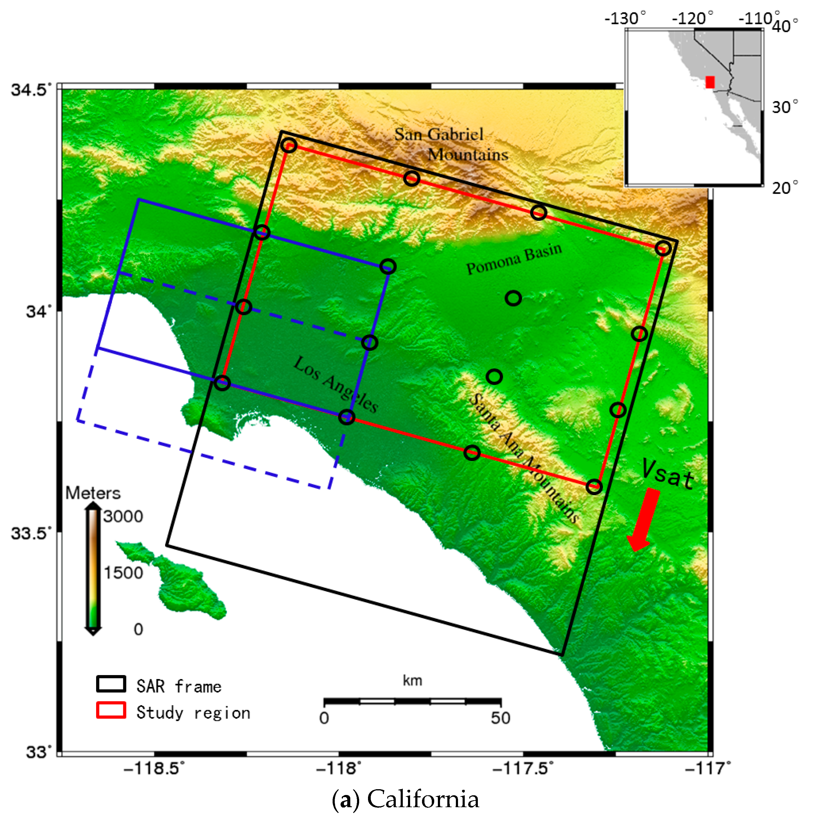
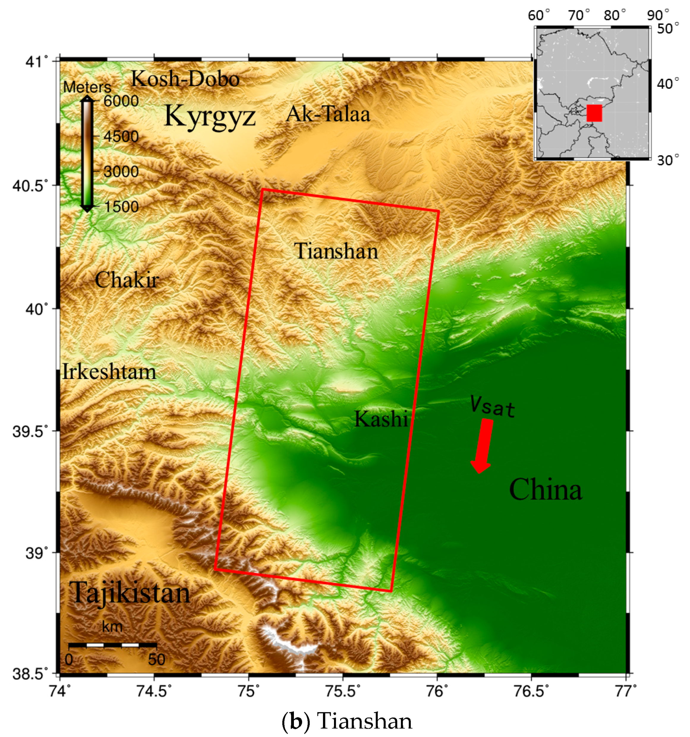
We investigated the correction capabilities of the PLE method on two test regions, Southern California and Tianshan. In California, we selected eight descending SAR images from the ENVISAT archives of the European Space Agency centered at 34° N, 117.8° W, covering an area of ~70 km by 100 km. These images were taken between 12 July 2008 and 25 September 2010 and were acquired on track 170 at 18:01 UTC (Figure 1a). The images extend from the San Gabriel Mountains (range of ~3 km elevation) in the north to the Los Angeles Basin area in the south. Significant and vertical surface displacements were revealed in the basin area (southern part of the interferogram) [37]. For the Tianshan region, we selected seven descending ENVISAT ASAR images on track 191, spanning the period from September 2007 to June 2010 and covering an area of ~80 km by 200 km (Figure 1b). The topography ranges from approximately 1 km to 6 km, extending from the South Tianshan Orogenic Belt to the Kashi area. The Kashi Depression is one of the most complex active tectonic areas in the southern flank of Tianshan, China. In the interseismic deformation rate map showing the Kashi Depression area between 2003 and 2007 obtained by InSAR time series analysis [38], no significant earthquakes occurred during our study period.
By selecting two different study areas, we can test and assess our PLE method under different geographical regions and atmospheric conditions. The test region in Southern California lies to the east and northeast of the Pacific Ocean and therefore has a humid atmosphere rich with atmospheric water vapor, which leads to a dominant stratified delay in the interferogram. Meanwhile, the test region in Tianshan in Northwestern China is an inland plateau with a semi-arid environment and a complicated atmospheric process. The atmospheric condition in this region is more turbulent than that in Southern California. We will discuss the performance of our PLE method under these two atmospheric conditions in Section 3. In addition, the deformation signals in the two study regions have different features: the deformation in California is mainly local, small-scale (<5 km) land subsidence in Los Angeles whereas, in Tianshan, the deformation is mainly large-scale (>10 s km) tectonic deformation. The different deformation characteristics also affect the band filtering, leading to selection of different bands, as discussed in Section 2.3.
For interferometric processing, we used the Repeat Orbit Interferometry Package (ROI_PAC) to focus the raw data and used DORIS to generate interferograms [39,40]. During processing, we used the precise ODR orbits from the Delft Institute for Earth-Oriented Space Research to minimize the orbital errors and the Shuttle Radar Topography Mission (SRTM) digital elevation model (30 m) to remove topographic phase [41]. The differential interferogram was corrected with a plane trend in the range and azimuth directions for residual orbital errors. All interferograms were multi-looked by 40 looks in azimuth and 8 looks in range to reduce phase noise and enhance phase unwrapping accuracy. Before phase unwrapping, the adaptive power spectrum filter was applied to improve the signal-to-noise ratio of the interferograms [42]. Finally, we obtained five interferograms in California and four interferograms in Tianshan for our case study and show the spatiotemporal baseline and coherence parameters in Table 1. We then used a coherence threshold of 0.2 to select coherent pixels, i.e., pixels with coherence values lower than 0.2 were discarded. Our test cases had small land deformation signals because of the short temporal baseline. Therefore, the dominant signals in the interferograms are contributed by tropospheric delay.
Global and regional reanalysis products provide estimates of atmospheric parameters several times a day at different pressure levels. We used the free archived ERA-I model, the latest global atmospheric reanalysis product from ECMWF, which is produced based on a 4D variable assimilation of global surface and satellite meteorological data. ERA-I provides data (pressure, temperature, and relative humidity) at a spatial resolution of 0.7° grid (~75 km), at a 6-h interval (0:00, 6:00, 12:00 and 18:00 UTC) daily, and on 37 pressure levels from 1989 to the present [27]. Figure 2 shows the distribution of ERA-I grid points in the two study areas.
2.2. Tropospheric Delay in InSAR Data
A tropospheric delay can be split into hydrostatic, wet, and liquid components depending on variations in atmospheric conditions. The wet component is the major limiting factor due to water vapor instability in space and time (approximately 20 mm to 300 mm) [43]. Unlike the wet delay, temperature and pressure are smooth in space, leading to a better-resolved, longer wavelength hydrostatic delay, accounting for about 90% of the total tropospheric delay (approximately 2.3 m in the zenith direction), but it stabilizes in time. The liquid component only becomes significant in a saturated atmosphere and is expected to be considerably small, measuring less than 0.1 mm/km to 0.4 mm/km under usual weather conditions for the C-band SAR system [9]. We focused only on the hydrostatic and wet delays, disregarding the effect of the water content in clouds [7]. The total zenith one-path tropospheric delay can be derived by the integration of air refractivity between the ground and the top of the troposphere (typically 15 km), above which the delay is assumed to be nearly negligible. The zenith hydrostatic and wet delays were projected to the line of sight (LOS) direction, which is expressed as follows [36]:
where is the summation of the hydrostatic delay and the wet delay , the incidence angle of the ray, the total atmospheric pressure, the partial pressure of water vapor in hPa, and the temperature in Kelvin. and indicate the dry air and water vapor specific gas constants [44]. The coefficients ,, and are empirical constants [45]. Geopotential height, temperature, and relative humidity were extracted from ERA-I reanalysis at each SAR acquisition. We then converted the geopotential height to a regular vertical metric grid by mapping () with latitude. The partial pressure was estimated from the relative humidity by a mixed Clausius–Clapeyron law as shown in the following equations [21].
where represents the partial pressure of saturation water vapor, is the relative humidity, provides the Clausius–Clapeyron law “over water“, and gives the Clausius–Clapeyron law “over ice“. Over , is used, and under , is used and a weighted average of both is used in between. The parameter values are , , , , and .
Providing meteorological parameters such as temperature, pressure, and water vapor partial pressure, we can use Equations (1)–(3) to calculate the relative tropospheric delay for interferograms generated from SAR acquisitions acquired at time and (Equation (6)). Thus, the relative tropospheric phase delay for the interferograms is easily derived by differentiating delays at acquisition times and , as shown in Equations (6) and (7).
In California, we used ERA-I outputs acquired at 18:00 UTC, which has a negligible difference with the SAR acquisition (18:01 UTC). In Tianshan, we selected ERA-I outputs at 00:00 UTC and 06:00 UTC, which are closest to the SAR acquisition (05:12 UTC). The linear interpolation in time was applied to obtain the corresponding delay at the SAR acquisition. By using Equations (1)–(5), we compute the total tropospheric delay on each ERA-I grid point within the blue rectangle in Figure 2. The resulting vertical profiles of delay are vertically interpolated using a spline interpolant and horizontally interpolated to each pixel in the SAR scene using a bilinear interpolant. Finally, we obtain the relative tropospheric delay for the interferogram by differentiating delay maps at each SAR acquisition (Equations (6) and (7)). Time and space interpolations, which can introduce uncertainties into delay corrections, are needed because of the low spatiotemporal resolution of the ERA-I model. However, our proposed PLE method is a phase-based method that estimates atmospheric contributions from the interferometric phase itself. Thus, an interpolation such as that in the ERA-I method is not required, avoiding the uncertainties introduced by poor interpolation. The details of the derivational processes and our corresponding strategies for data processing are discussed in the following subsections.
2.3. Power Law Model Based on ERA-I Reanalysis (PLE)
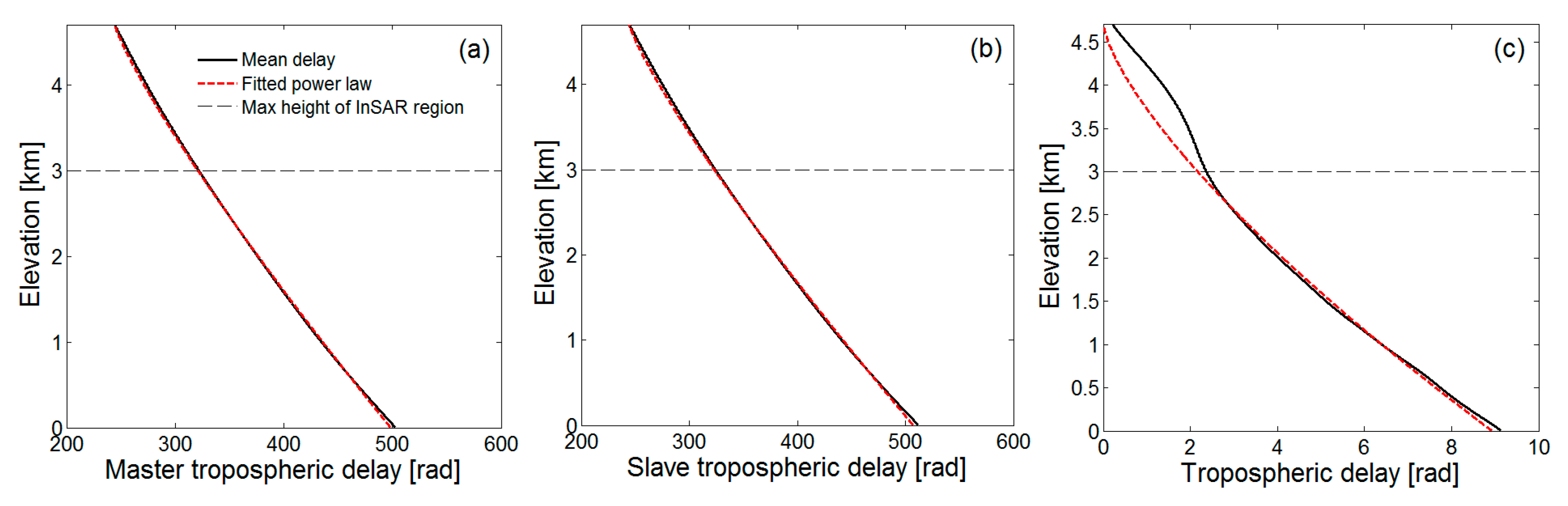
The relationship between the absolute tropospheric delay and elevation can be illustrated by a power law model, as shown in Equation (8) [35]. Similar to Bekaert et al. [35,36], we estimate and from the tropospheric delay curves. is the slope of the mean delay curve in the log-log domain and is the constrained height where the standard deviation and average value of the relative delays are both smaller than 1.0 rad (~0.45 cm). Figure 3 shows the vertical profile of the tropospheric delay in the California test region estimated using ERA-I reanalysis on six grid points located in the green rectangle in Figure 2a. The absolute tropospheric delay at SAR acquisitions 20090627 and 20090905 are shown in Figure 3a,b. The relative tropospheric delay () on the interferogram formed by these two images is shown in Figure 3c. By plotting the mean relative tropospheric delay (black solid line) against the reference elevation [], we can determine the power law relationship (red dashed line) indicated by the linear pattern.
where is a scaled factor that relates tropospheric delay to topography, is the coefficient describing the power law model estimated by ERA-I reanalysis, and is the phase delay at , indicating the relative phase-delay offset on an individual interferogram.
Figure 3c shows that at a specific altitude (~5 km) the relative delays converged but the delays at master and slave acquisitions did not. The difference in was found to be considerably small and the average value (~1.2) was often used when using the power law method. However, in many cases, the average could not indicate the relationship between the phase and topography because the interferometric phase is the phase difference between the master and slave acquisitions. Thus, tropospheric delay depends on the change in refractivity rather than the absolute refractivity in each acquisition. The differences in among different interferograms was found to be as high as 0.2 in our case, leading to a relative tropospheric delay change in 10 s of rad. To address this problem, we directly estimated on each interferogram from the ERA-I reanalysis. Similar to the absolute tropospheric delay at SAR acquisition, the relative tropospheric delay on the interferogram also decreases with elevation and does not change significantly and converged when a certain height is reached. Thus, the tropospheric delay above this constrained height is negligible.
After estimating the power law relationship, we set at a fixed value by controlling the offset . was also estimated by plotting the slope of the log-log relationship between phase and topography, which were the constants for a given interferogram. However, the scaled factor is not a constant for an entire interferogram and is not easy to estimate due to the spatially variable tropospheric delay.
Interferometric phases are a superposition of multiple signals, including tropospheric delay, deformation, and residual orbit errors, in which wavelengths contain a multi-scale dependent spectrum and may have different sensitivities to one another. For example, tropospheric signals contain short wavelength-scale (few kilometers) components and are introduced by turbulent components in the troposphere. Long wavelength-scale (tens of kilometers) components are introduced by hydrostatic and wet delays due to weather condition variations and are partly correlated with topography. In addition, longer wavelength-scale (hundreds of kilometers) components introduced by ground deformation such as tidal loading, tectonic slow slip, or earthquakes may be more sensitive to other sources of confounding noises. Therefore, the selection of the band filter is not always trivial, as it requires empirical information about multi-scale dependent spectrums. However, we took advantage of the fact that the tropospheric signal is present at all wavelength scales to estimate the scaled factor from a spatial frequency band that was relatively insensitive to the other signals [33]. Similar to the original power law method [35,36], band filtering was applied to the phase and topography to select an appropriate band such that other phase contributions were negligible. Thus, we can modify Equation (8) into the following [35]:
where is the tropospheric delay fitted by the band-filtered phase and reference height . in Equation (9) is the elevation of pixels extracted from SRTM DEM and in Equation (8) is the elevation of the ERA-I outputs. is the constrained height. is the local scaled factor estimated in a moving window for an interferogram. is the spatially variable factor calculated by multi-weighted . The band filtering would not change the scaled factor estimates only if there are contaminated signals. is the final estimated tropospheric delay on interferograms. was estimated based on ERA-I reanalysis.
To introduce band-filtering artifacts conveniently, we removed the initial shift from interferometric phases. This shift was a long wavelength component that was filtered out later. We estimated the shift from interferometric phases over multiple windows, which varied in space and was influenced by other phase contributions. Therefore, in many cases, the shift cannot exactly represent the tropospheric delay offset and cannot be estimated from a spatial band that is insensitive to other phase signals.
Finally, we used Equation (9) to estimate the local factor between the band-filtered phase and topography, where the band was selected such that the contribution from other signals was negligible. Accounting for spatially variable tropospheric delays, we applied a moving window to the interferogram. The window was moving from the bottom to the top in the azimuth direction and from the left to the right in the range direction (Figure 1a). Over each window, the local band-filtered phase-topography relationship was analyzed and was estimated. The local robust estimation of plays a critical role in increasing the accuracy of tropospheric delays. An expanded robust technique was used to estimate in each window, which can reduce the sensitivity to outliers (e.g., due to residual deformation signal or other measurement error sources) [46]. The error equation can be constructed based on Equation (9) as follows:
where , and represent the random error, band-filtered phase, and a constant shift for the ith pixel on a local window, respectively. N represents the number of pixels on the local window.
The parameter estimator can be derived based on the adjustment principle of least squares, as follows:
where represents the equivalent weight matrix of the vector L. The ith diagonal element of is calculated by . is the corresponding weight factor calculated by the function of IGGIII [47]. The parameters can be robustly and reliably estimated by an expanded robust estimation [46] given that the initial value of the equivalent weight matrix was set. When the parameters are estimated, the covariance matrix of the estimates can be obtained through variance propagation in Equation (12) as follows:
where is the corresponding variance factor of the unit weight.
When the of each window was estimated, a multiple weighted and extrapolated method was applied to all pixels in the interferograms. The multi-weighted function was constructed with the STD of the estimate and the distance from the window centers to each pixel (Equations (14)–(16)).
where S represents the reformed weights of the STD from the robust estimation (Equations (13)). G represents the Gaussian distribution based on the distance. is the ith STD of in the ith window. The multiple weights W are a matrix. is the final derived scaled factor for all pixels in Equation (10). N is the number of pixels, and n is the number of windows for the entire interferogram. Figure 4 shows the flow chart of the PLE method on the interferogram.
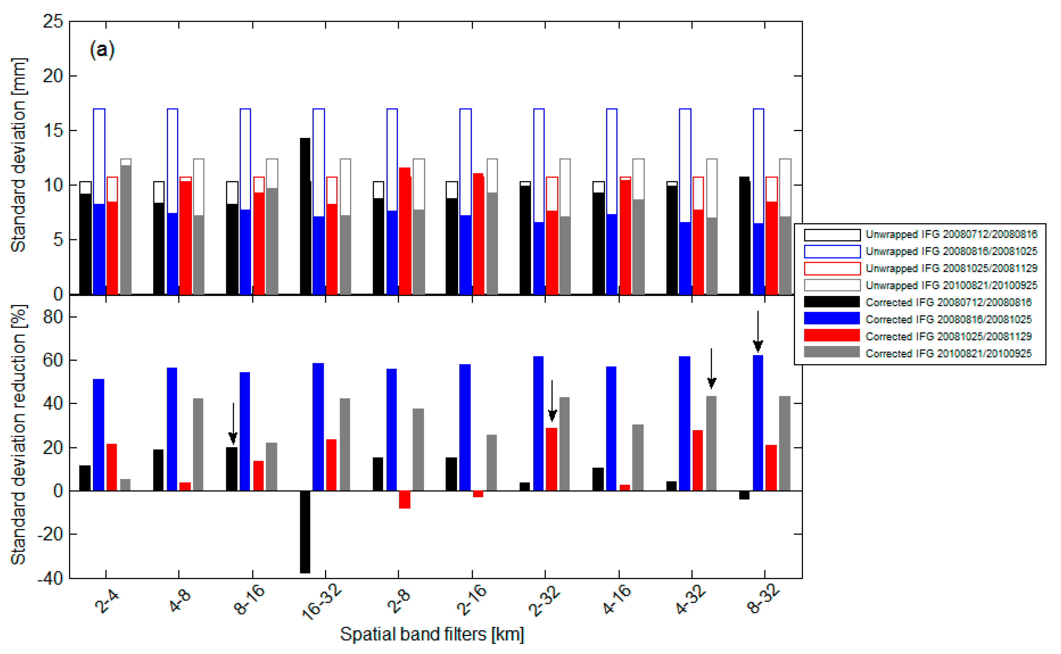
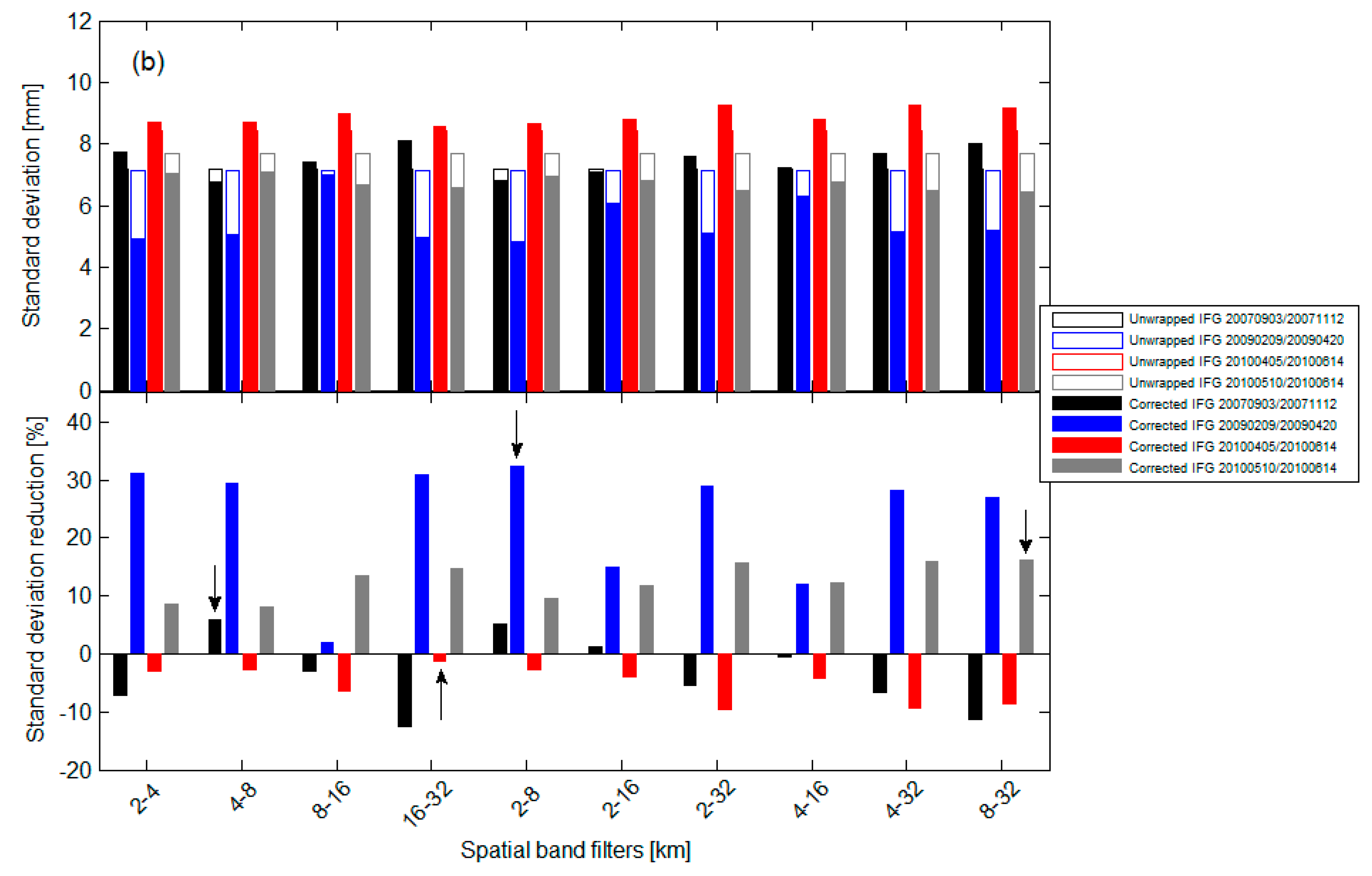
The PLE method can account for lateral variations in space by estimating in multiple windows and can be applied in regions without removing a preliminary deformation [33]. The robust estimation technique is always available in each study area for a given day at a closet SAR acquisition. However, the selection of the band filter is not always trivial because it requires empirical information on multi-scale dependent spectrums. A potential option is to perform a statistical analysis of multiple spatial bands to select the appropriate bands. We compared the mitigation results of multiple bands with the corresponding unwrapped interferograms, expecting the largest reduction in STD if this band exhibits the best performance. The STD for each interferogram before and after correction using the PLE method by different spatial band filters is shown in Figure 5. The STD significantly varies between different bands in California (mean STD of 8.6 mm) than in Tianshan (mean STD of 7.1 mm). The arrows in Figure 5, which were selected for each interferogram, represent the bands with the largest reduction in STD. The spatial band-filtering approach relies on the manifestation of tropospheric delay at all spatial scales; often, the deformation signal may be at specific spatial wavelengths. However, determining the spatial bands, which are the representatives of the tropospheric delay, can be challenging. Apart from the deformation signal, turbulent and coherent tropospheric features, DEM errors, and orbital errors, which contaminate the spatial bands, can also be observed. Therefore, different deformation features, atmospheric conditions, possible DEM errors and orbit errors for different interferograms, as well as different topographic variations for different study regions lead to the different spatial bands, as selected in Figure 5.
3. Results and Discussion
We applied our proposed PLE method to the Southern California and Tianshan study areas and compared tropospheric corrections estimated from the linear and ERA-I methods. Accuracy was evaluated by using the unwrapped SAR interferograms and validated by comparing the delay measurements from the passive multispectral imager MERIS onboard the ENVISAT satellite.
3.1. Estimation of PLE Parameters
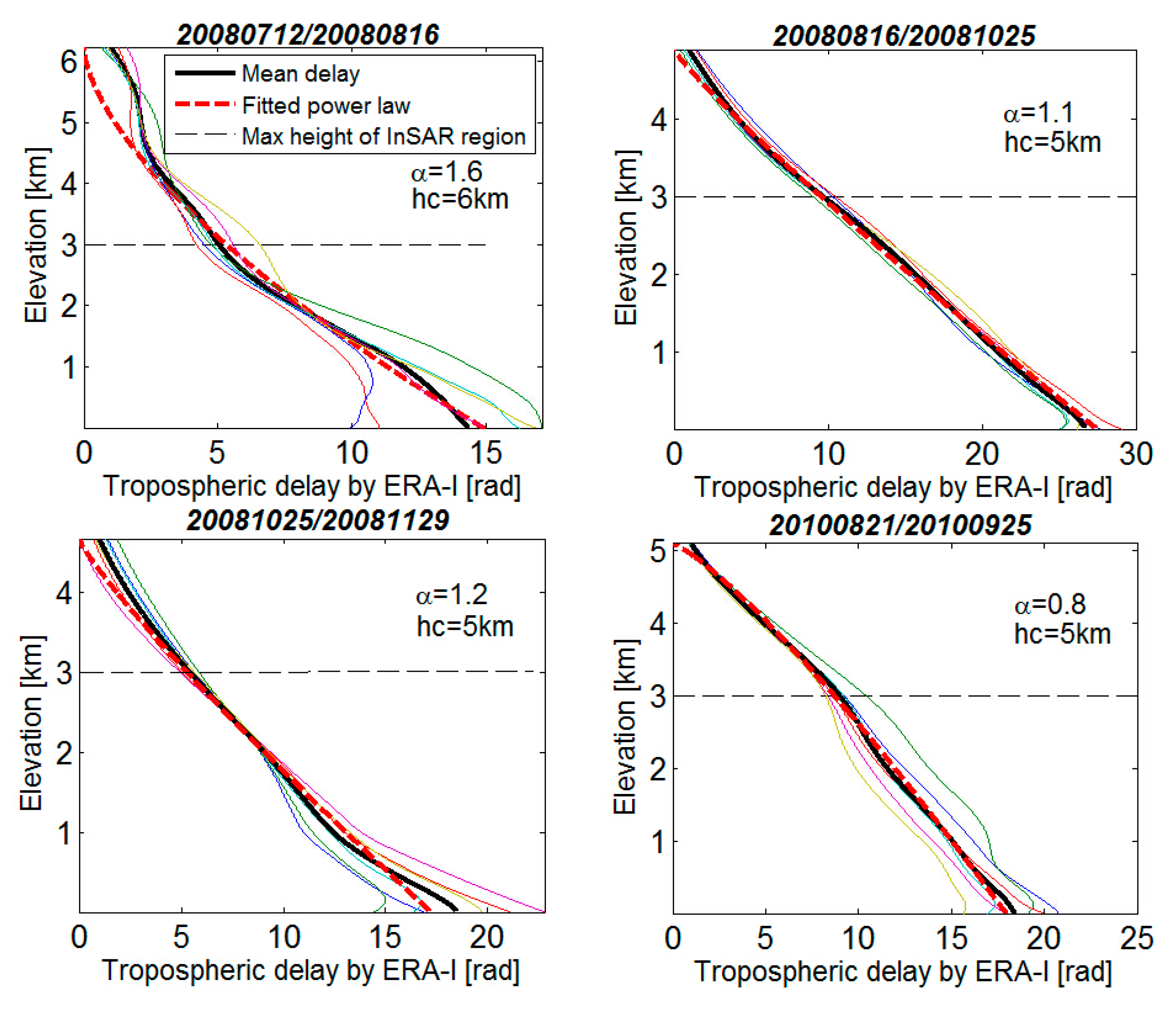
The study by Bekaert et al. [35] assumed that and are constants for the study region and for each interferogram and estimated them by using sounding data. In our study, we assumed that the coefficients change with time (i.e., they are different for each interferogram), and instead of sounding data, we used ERA-I reanalysis to estimate these two coefficients, as shown in Figure 6. The relative delay curves can be fit by a power law function, and the coefficients vary with different interferograms. The success of the PLE method is limited to the cases in which the relative delays can be reasonably approximated by a power law function.
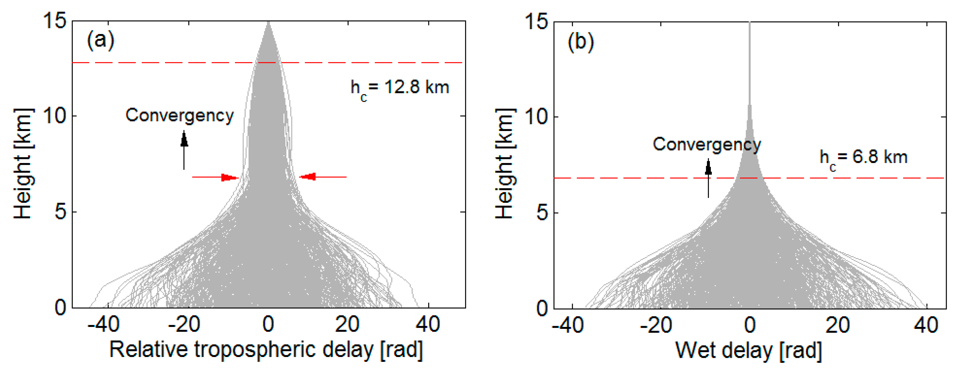
The sounding data have extremely low spatiotemporal resolution (only provide data twice per day). ERA-I reanalysis provides data at a relatively high spatiotemporal resolution (at six-hour intervals daily). Therefore, we can estimate the two coefficients from the statistical results of the tropospheric delay difference based on spatial variation, the values of which are estimated for each specific SAR acquisition. We used ERA-I reanalysis to calculate the relative delay curves at six grid points (the red points inside the green rectangle in Figure 2a), and determine by constraining the STD and average value. Then, we used the mean relative curves to estimate by fitting a power law function. As shown in Figure 7, we set from the statistical results of the combinations of relative delay curves (difference of delay at two different days). Relative tropospheric delays (hydrostatic delay + wet delay, shown in Figure 7a) and wet delays (Figure 7b) are computed from ERA-I reanalysis in California for 120 days (18:00 UTC) between June and October 2009. The data could empirically represent the delays for interferogram 20090627/20090905 (example in Figure 3). The relative delays did not change significantly at a certain height (red arrows) and converged (red dashed lines) at a specific height of 12.8 km (Figure 7a); wet delays converged at the height of 6.8 km (Figure 7b). The constrained height for total tropospheric delays was higher than that for wet delays. This case shows that hydrostatic delays affected the estimation of the constrained height and cannot be simply ignored in the interferograms. However, the relative delays have an obvious tendency to converge at a certain height (indicated by red arrows in Figure 7a); this height value is extremely close to the convergent height for the wet delays, as shown in Figure 7b. Therefore, we set the constrained height to ~5 km, which is lower than the temporal statistics of the tropospheric delays, but near the wet delays. In our experiment, the constrained heights, which are specifically estimated from ERA-I reanalysis by spatial statistics, are generally lower than the global results from temporal statistics.
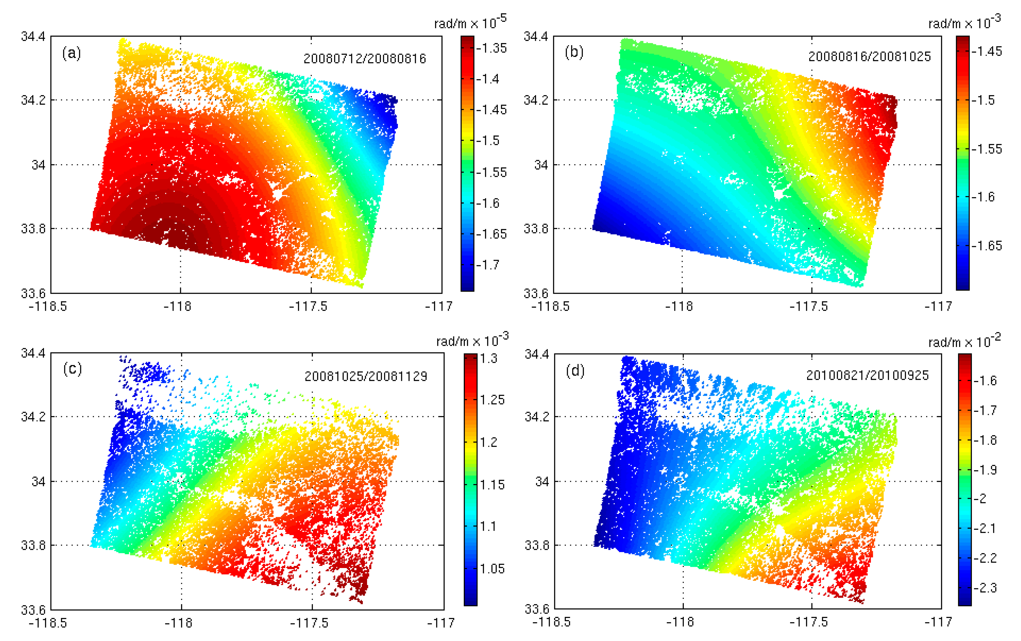
The local robust estimation of the scaled factor in each window plays a critical role in increasing the accuracy of tropospheric delays. As described in Section 2.3, we used a robust technique to estimate to avoid the impact from outliers. We can account for the spatial variation of tropospheric delay by applying the PLE method. The spatial variation maps of are shown in Figure 8. The PLE method splits the study region into 16 blocks with an overlap area of 50% in our study. The partially overlapping windows can reduce edge effects and ensure adjacent consistency.
To verify the effectiveness of our robust estimation method, we tested the approach on InSAR data from interferogram 20081025/20081129 in California. The dataset is shown in Table 1. The interferometric phase and the reference height are both band filtered in the 2–32 km spatial wavelength. We calculated the STD of the scaled factor estimates by assuming a linear model using the least squares and robust estimation methods. Although the dominant signals in the original band-filtered phases are contributed by topographically-correlated tropospheric delays, we can still detect some outlier rejection phases (72, indicated by red points in Figure 9a). The improvement in the STD values is ~10%. As shown in Figure 9b, we applied these two methods to the original band-filtered data with extra simulated outliers (200), which are randomly introduced to the locations. We detected 248 outlier rejection phases (recognition rate is ~91%, indicated by red points in Figure 9b), which do not contribute in estimating the scaled factor. The improvement of STD is ~15%. Figure 9c shows the relationship between improvement of STD and pollution rate of the data. Before a specific outlier percentage (~22%, indicated by the arrow in Figure 9c), the improvement of STD consistently increased with increasing outlier percentage. Then, when the outlier percentage is high, the improvement of STD decreases. When the outlier percentage is close to ~50%, the least squares regression and robust estimation would be ineffective. These results suggest that the robust estimation method yields the scaled factor robustly and reliably.
3.2. Estimation of Tropospheric Delays
We evaluated the performance of our PLE method through a comparison with the conventional linear and ERA-I methods. In addition, the accuracy was validated with the MERIS in California [16]. We implemented the linear, ERA-I, and MERIS corrections, which are included in TRAIN. No MERIS data are available for comparison in Tianshan. MERIS-derived delay prediction is only used when the cloud coverage is less than 20% of SAR scene. The map of tropospheric wet delay was calculated from the MERIS precipitable water vapor (PWV) as follows:
where is conversion factor given by Bevis et al. [48] as
where is the density of liquid water, is the ratio of molecular masses of water vapor and dry air (), and is the weighted average of the temperature between the ground and reference height, as follows:
We evaluated the at each pixel of interferogram using the atmospheric outputs from ERA-I to produce a map of . We then calculated the tropospheric wet delay by multiplying the MERIS PWV by , as shown in Equation (17). Values of that typically range from 5 to 7 with an average value of 6.2 are usually adopted [16]. To validate our approach, we also added the hydrostatic delay derived from ERA-I to the MERIS wet delay to determine the total tropospheric delay.
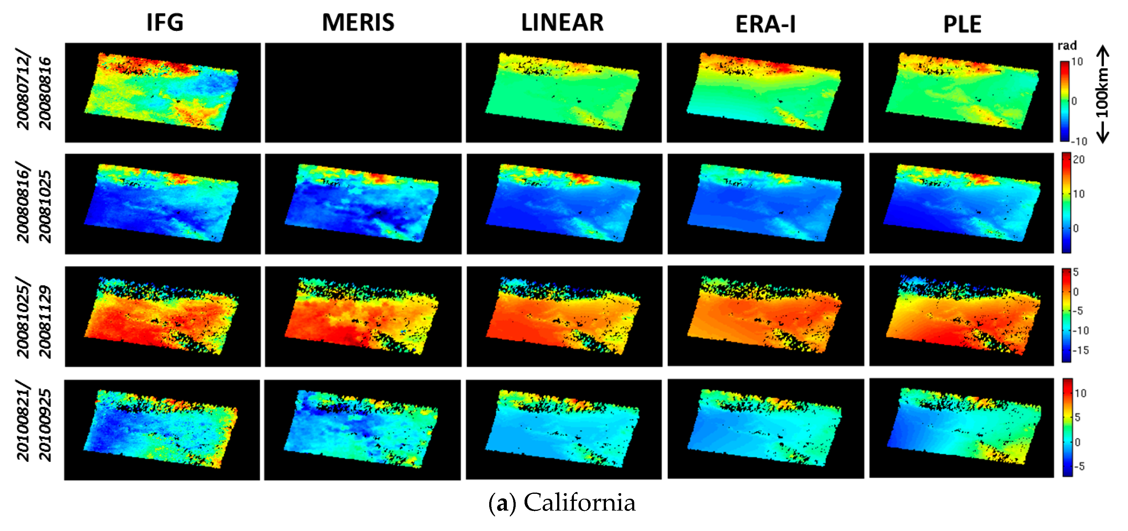
Figure 10 shows examples of the tropospheric delays produced from the four methods for each test region. The interferograms are mainly caused by tropospheric delays, which are topographically correlated. The tropospheric delay is the sum of two components, namely, stratified delay and turbulent delay. The stratified delay is the result of different vertical refractivity profiles from the two SAR images; it mainly affects mountainous terrain and shows a strong correlation with topography. The turbulent delay results from turbulent processes in the atmosphere and affects flat terrain as well as mountainous terrain. The spatiotemporal filtering in InSAR time series methods cannot estimate the tropospheric delay because the seasonality of delay is underestimated [21]. Therefore, we used the PLE method to estimate the stratified delay for each individual interferogram. The PLE method, however, similar to all phase-based methods, is not suitable in cases where significant turbulence mixing occurs. Therefore, we only focus on estimating the topographically correlated tropospheric delay that often dominates the tropospheric signal on an interferogram. The linear method () assumes a simple phase-topography relationship for the entire interferogram; therefore, it does not allow for spatially variable tropospheric delay.
Figure 10 shows that all these methods indicate delays with similar spatial distribution and magnitude. Discrepancies can also be observed between the four estimated tropospheric delays in California and Tianshan. MERIS-estimated tropospheric delays show a strong resemblance to the unwrapped interferograms because they were acquired simultaneously with ASAR images with high precision. The ERA-I method shows delays with an accurate location, but not always with a similar order of magnitude (e.g., interferogram 20100405/20100614 in Tianshan). This condition is partly due to an inaccurate interpolation of the ERA-I reanalysis outputs. The phase-based methods (the linear and PLE) assume a phase-topography relationship; thus, they are incapable of capturing turbulent signals. Although the ERA-I method can capture the spatial trends of tropospheric delay accurately in a region, this method cannot capture the higher gradients in the turbulent delay (e.g., interferogram 20080712/20080816 in California). MERIS delays, shown in Figure 10a, also contain the hydrostatic component estimated from ERA-I, allowing for comparison with the phase-based methods. The hydrostatic delay component is related to the ratio of atmospheric pressure P and the surface temperature T at the scale of an interferogram (typically 100 km). The spatial variations of pressure are usually small, typically at an order of magnitude of 1 hPa, whereas larger variations in water vapor partial pressure are common. Consequently, the differential wet delay usually overwhelms the differential hydrostatic delay on the interferogram. Therefore, most correction methods focused on estimating the wet delay. Doin et al. [49] validated the seasonal change in hydrostatic delay with temperature in seasonal fluctuations and pointed out that hydrostatic delay must be considered when the change in the local temperature is more than 10° within one year. Figure 11 shows the relation between height and hydrostatic delay estimated using ERA-I method and the magnitude of hydrostatic delays can reach 1 rad. This condition demonstrates that the hydrostatic delay cannot be simply ignored on the interferograms.
3.3. Statistical Comparison of Tropospheric Correction Methods
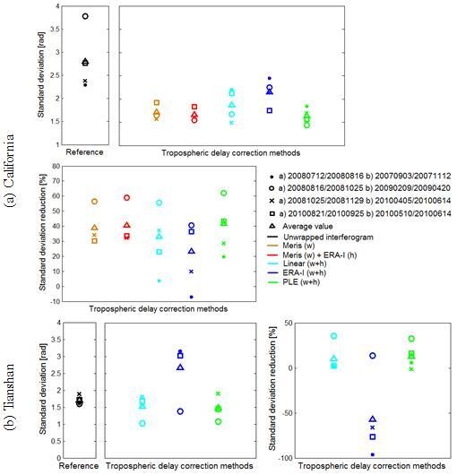
We performed a statistical analysis to compare tropospheric delays estimated from the four correction methods (MERIS, the linear, ERA-I, and PLE methods) to the unwrapped interferograms. In Figure 12, we performed the comparison by plotting the interferometric phase before and after correction against the elevation for interferograms presented in Figure 10. Figure 12a shows that all these methods were effective in mitigating topographically correlated tropospheric delays in California. The slope between the corrected phases and elevation reduced in all correction methods. However, limited improvements were found in Tianshan, as shown in Figure 12b because the tropospheric delays do not show a strong relationship with topography, and might have mainly resulted from the turbulent delay. After using ERA-I for corrections, the results even deteriorated due to the low spatial resolution of the reanalysis, indicating that ERA-I could introduce atmospheric estimation error into the final displacement results because of the uncertainties produced by the interpolation operation. However, the PLE method always yielded effective delay mitigation, as shown by STD reduction after tropospheric correction using the three different tropospheric techniques. We expect a high STD reduction when a method performs efficiently. As shown in Figure 13, the left panel shows the STD of the unwrapped interferograms, whereas the right panel shows the residual STD after correction using the different tropospheric estimation methods.
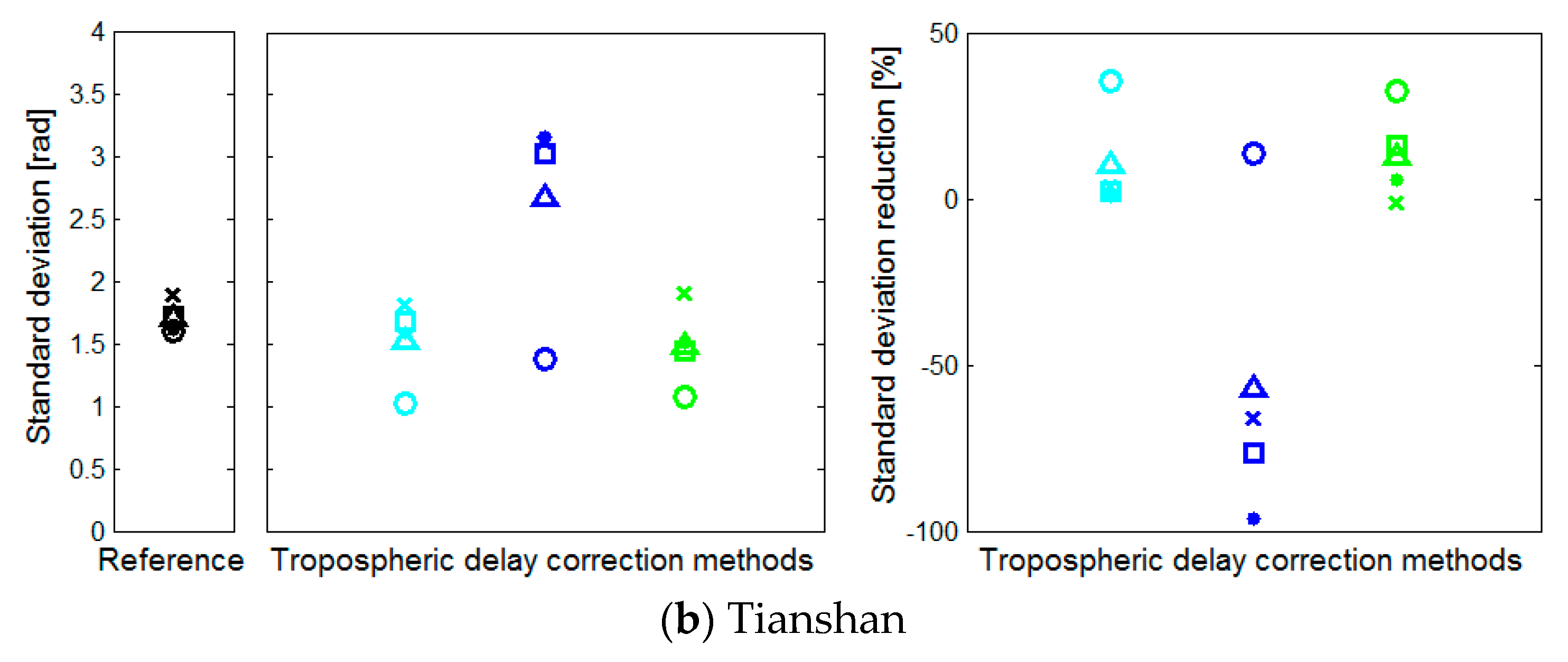
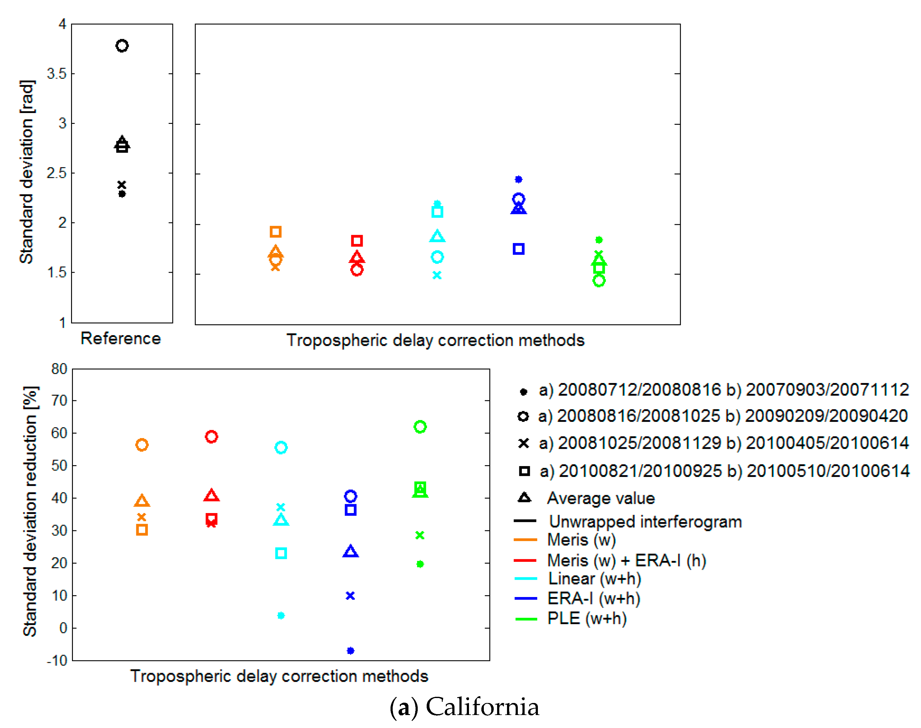
In California, all methods are effective in mitigating tropospheric delays, leading to STD reduction. MERIS, on average, provides better STD reduction (~41%) than the linear method (~33%) and ERA-I (~23%). The MERIS results in STD reduction are approximately equal to the MERIS ~1.8 rad accuracy level computed using the measured ~1.1 mm PWV accuracy (brown symbols in Figure 13a) [16]. Moreover, MERIS delays containing hydrostatic component from ERA-I showed better reduction (average value was ~2%) than those without hydrostatic component. The average STD reduction of the residuals after correction using MERIS without and with hydrostatic delay is ~39% and ~41%, respectively. Therefore, we cannot simply ignore the hydrostatic delay effect. Unlike ERA-I, no uncertainty is introduced through temporal interpolation for MERIS because MERIS measurements were acquired simultaneously with ASAR images. Figure 13a shows that ERA-I yielded an average STD reduction of ~23% (blue symbols), which was the worst among the four methods. This result was probably due to the low spatial resolution. The phase-based methods, mainly designed to resolve the topographically correlated delay, can retrieve the tropospheric delay; the PLE and the linear methods provide an STD reduction of ~42% and ~33%, respectively. Thus, the PLE method performed better than the linear method because the PLE method can account for the spatial variation of tropospheric delay, whereas the conventional linear model cannot. The tropospheric delays in the region of California are mainly the stratified delays that are strongly correlated with topography (also shown in Figure 12a). Thus, the phase-based methods performed well in this area. The PLE method given that it is applied locally is more subjected to contamination from various tropospheric delay components present at different spatial scales than the global linear method. For example, for the interferogram 20081025/20081129, the STD reduction is ~37% after the linear correction, whereas the reduction is ~29% after the PLE method. Considering that both phase-based methods have the potential to introduce inaccurate signals in the presence of serious turbulence and coherent short-scale tropospheric signals, neither of them should be applied in those cases.
In Tianshan, MERIS-derived tropospheric delays were not available for comparison. We did not observe an improvement when using ERA-I except for interferogram 20090209/20090420 (blue symbols in Figure 13b). On average, STD increased (increase ~57%) rather than decreased after correction using ERA-I. The two possible reasons for this deterioration are as follows. First, the requirement for temporal, lateral, and vertical interpolations of the atmospheric parameters introduces uncertainties into the delay estimations. Second, the turbulent process in the atmosphere in Tianshan often appears due to the high altitude and complicated terrain. Parts of the tropospheric delays on the interferograms are mainly the small-scale turbulent delay, which cannot be captured by ERA-I. For phase-based methods, we found slight improvements, with an average reduction in STD of ~10% and ~13% for the linear and PLE methods, respectively.
In conclusion, the PLE method outperforms the linear and ERA-I methods in the regions where tropospheric delays are correlated with topography, and agrees well with MERIS measurements. Moreover, the success of our PLE method is limited to the cases in which the relative delays can be reasonably approximated by a power law function. The main limitation of the robust estimation technique in the PLE method is that the algorithm should be implemented iteratively; thus, its computational efficiency is lower than that of least squares regression. From our analysis, each method has its limitations, which vary with the region of application and with time. In future work, we will identify suitable metrics and combine different tropospheric estimation methods, which could further improve the accuracy of InSAR processing.
4. Conclusions
We developed and tested a method to estimate the tropospheric delay in radar interferogram using a power law model based on ERA-I reanalysis. The PLE method is a modification of the power law method proposed by Bekaert et al., which mainly has two novelties: one is that the power law coefficients are estimated using ERA-I reanalysis instead of the sounding data, which is usually available in a study region; the other is that the scaled factor is estimated using the robust estimation technique instead of least squares regression, which is outlier-resistant. To separate deformation and tropospheric signals, a frequency band insensitive to deformation is tested and selected in the study. The PLE method splits a region into multiple blocks (approximately 100 km2 in our study) and estimates the scaled factor robustly to capture the spatial variations of tropospheric delay in lager regions. We tested the PLE method on ENVISAT ASAR images in Southern California and Tianshan, which have different geographical regions and atmospheric conditions. In our study regions, the iterative calculation approach applied in the PLE method is relatively straightforward and efficient when estimating tropospheric delay.
We performed a comparison of the tropospheric corrections estimated from the conventional linear, independent ERA-I, and PLE methods. The accuracy was evaluated by corrected SAR interferograms and was validated by using MERIS measurements. After correction, our PLE method had greater reduction in the topographically correlated tropospheric signals than the conventional linear and ERA-I methods. Moreover, our method improved the agreement with delay measured from MERIS. The success of the PLE method is limited to cases in which the relative delays can be reasonably approximated by a power law relationship between topography and phase. The main limitation of the robust estimation technique in the PLE method is that the algorithm should be implemented iteratively; thus, its computational efficiency is lower than that of least squares regression. Each method has its limitations in different regions and at different times. Therefore, in some cases, different tropospheric estimation methods should be combined due to the complicated geological structure of the earth and the variability in the atmospheric circulation.
Acknowledgments
We greatly appreciated three anonymous reviewers for their valuable comments and thank David Bekaert for providing TRAIN (Toolbox for Reducing Atmospheric InSAR Noise) package. We greatly appreciated the financial supports from the National Natural Science Foundation of China (No. 41404028) and the National Basic Research Program of China (No. 2013CB733300).
Author Contributions
Bangyan Zhu designed the proposed approach and performed the experiments. Jiancheng Li supervised all work. All authors evaluated the results and wrote the paper.
Conflicts of Interest
The authors declare no conflict of interest.
References
- Massonnet, D.; Holzer, T.; Vadon, H. Land subsidence caused by the East Mesa geothermal field, California, observed using SAR interferometry. Geophys. Res. Lett. 1997, 24, 901–904. [Google Scholar] [CrossRef]
- Colesanti, C.; Wasowski, J. Investigating landslides with space-borne Synthetic Aperture Radar (SAR) interferometry. Eng. Geol. 2006, 88, 173–199. [Google Scholar] [CrossRef]
- Lanari, R.; Lundgren, P.; Sansosti, E. Dynamic deformation of Etna Volcano observed by satellite radar interferometry. Geophys. Res. Lett. 1998, 25, 1541–1544. [Google Scholar] [CrossRef]
- DiCaprio, C.J.; Simons, M. Importance of ocean tidal load corrections for differential InSAR. Geophys. Res. Lett. 2008, 35. [Google Scholar] [CrossRef]
- Bekaert, D.; Hooper, A.; Wright, T. Reassessing the 2006 Guerrero slow slip event, Mexico: Implications for large earthquakes in the Guerrero Gap. J. Geophys. Res. Solid Earth 2015, 120, 1357–1375. [Google Scholar] [CrossRef]
- Zebker, H.A.; Rosen, P.A.; Goldstein, R.M.; Gabriel, A.; Werner, C.L. On the derivation of coseismic displacement fields using differential radar interferometry: The Landers earthquake. J. Geophys. Res. Solid Earth 1994, 99, 617–634. [Google Scholar] [CrossRef]
- Gray, A.L.; Mattar, K.E.; Sofko, G. Influence of ionospheric electron density fluctuations on satellite radar interferometry. Geophys. Res. Lett. 2000, 27, 1451–1454. [Google Scholar] [CrossRef]
- Zebker, H.A.; Rosen, P.A.; Hensley, S. Atmospheric effects in interferometric synthetic aperture radar surface deformation and topographic maps. J. Geophys. Res. 1997, 102, 7547–7563. [Google Scholar] [CrossRef]
- Hanssen, R. “Radar Interferometry”, in Data Interpretation and Error Analysis; Springer: Delft, The Netherlands, 2001. [Google Scholar]
- Li, Z.; Fielding, E.; Cross, P.; Preusker, R. Advanced InSAR atmospheric correction: MERIS/MODIS combination and stacked water vapour models. Int. J. Remote Sens. 2009, 30, 3343–3363. [Google Scholar] [CrossRef]
- Hooper, A.; Bekaert, D.; Spaans, K.; Arıkan, M. Recent advances in SAR interferometry time series analysis for measuring crustal deformation. Tectonophysics 2012, 514, 1–13. [Google Scholar] [CrossRef]
- Tang, W.; Liao, M.; Yuan, P. Atmospheric correction in time-series SAR interferometry for land surface deformation mapping—A case study of Taiyuan, China. Adv. Space Res. 2016, 58, 310–325. [Google Scholar] [CrossRef]
- Webley, P.; Bingley, R.; Dodson, A.; Wadge, G.; Waugh, S.; James, I. Atmospheric water vapour correction to InSAR surface motion measurements on mountains: Results from a dense GPS network on Mount Etna. Phys. Chem. Earth Parts A/B/C 2002, 27, 363–370. [Google Scholar] [CrossRef]
- Onn, F.; Zebker, H.A. Correction for interferometric synthetic aperture radar atmospheric phase artifacts using time series of zenith wet delay observations from a GPS network. J. Geophys. Res. 2006, 111. [Google Scholar] [CrossRef]
- Williams, S.; Bock, Y.; Fang, P. Integrated satellite interferometry: Tropospheric noise, GPS estimates and implications for interferometric synthetic aperture radar products. J. Geophys. Res. 1998, 103, 27051–27067. [Google Scholar] [CrossRef]
- Li, Z.; Fielding, E.J.; Cross, P.; Muller, J.-P. Interferometric synthetic aperture radar atmospheric correction: Medium Resolution Imaging Spectrometer and Advanced Synthetic Aperture Radar integration. Geophys. Res. Lett. 2006, 33. [Google Scholar] [CrossRef]
- Li, Z.; Xu, W.; Feng, G.; Hu, J.; Wang, C.; Ding, X.; Zhu, J. Correcting atmospheric effects on InSAR with MERIS water vapour data and elevation-dependent interpolation model. Geophys. J. Int. 2012, 189, 898–910. [Google Scholar] [CrossRef]
- Li, Z.H.; Muller, J.P.; Cross, P.; Fielding, E.J. Interferometric synthetic aperture radar (InSAR) atmospheric correction: GPS, moderate resolution Imaging spectroradiometer (MODIS), and InSAR integration. J. Geophys. Res. 2005, 110. [Google Scholar] [CrossRef]
- Puysségur, B.; Michel, R.; Avouac, J.-P. Tropospheric phase delay in interferometric synthetic aperture radar estimated from meteorological model and multispectral imagery. J. Geophys. Res. 2007, 112. [Google Scholar] [CrossRef]
- Foster, J.; Brooks, B.; Cherubini, T.; Shacat, C.; Businger, S.; Werner, C.L. Mitigating atmospheric noise for InSAR using a high resolution weather model. Geophys. Res. Lett. 2006, 33. [Google Scholar] [CrossRef]
- Jolivet, R.; Grandin, R.; Lasserre, C.; Doin, M.P.; Peltzer, G. Systematic InSAR tropospheric phase delay corrections from global meteorological reanalysis data. Geophys. Res. Lett. 2011, 38. [Google Scholar] [CrossRef] [Green Version]
- Gong, W.; Meyer, F.; Liu, S. Performance analysis of atmospheric correction in insar data based on the weather research and forecasting model. In Proceedings of the International Geoscience and Remote Sensing Symposium, Honolulu, HI, USA, 25–30 July 2010; p. 5. [Google Scholar]
- Nico, G.; Tome, R.; Catalao, J.; Miranda, P.M. On the use of the WRF model to mitigate tropospheric phase delay effects in SAR interferograms. IEEE Trans. Geosci. Remote Sens. 2011, 49, 4970–4976. [Google Scholar] [CrossRef]
- Liu, S.; Mika, A.; Gong, W.; Hanssen, R.; Meyer, F.; Morton, D.; Webley, P.W. The role of weather models in mitigation of tropospheric delay for SAR interferometry. In Proceedings of the International Geoscience and Remote Sensing Symposium, Vancouver, BC, Canada, 24–29 July 2011; p. 4. [Google Scholar]
- Walters, R.; Parsons, B.; Wright, T. Constraining crustal velocity fields with InSAR for Eastern Turkey: Limits to the block-like behavior of Eastern Anatolia. J. Geophys. Res. Solid Earth 2014, 119, 5215–5234. [Google Scholar] [CrossRef]
- Jolivet, R.; Agram, P.S.; Lin, N.Y.; Simons, M.; Doin, M.P.; Peltzer, G.; Li, Z. Improving InSAR geodesy using Global Atmospheric Models. J. Geophys. Res. Solid Earth 2014, 119, 2324–2341. [Google Scholar] [CrossRef]
- Dee, D.P.; Uppala, S.M.; Simmons, A.J.; Berrisford, P.; Poli, P.; Kobayashi, S.; Andrae, U.; Balmaseda, M.A.; Balsamo, G.; Bauer, P.; et al. The ERA-Interim reanalysis: Configuration and performance of the data assimilation system. Q. J. R. Meteorol. Soc. 2011, 137, 553–597. [Google Scholar] [CrossRef]
- Michalakes, J.; Dudhia, J.; Gill, D.; Henderson, T.; Klemp, J.; Skamarock, W.; Wang, W. The weather research and forecast model: Software architecture and performance. In Proceedings of the 11th ECMWF workshop on the use of high performance computing in meteorology, Reading, UK, 25–29 October 2004; pp. 156–168. [Google Scholar]
- Delacourt, C.; Briole, P.; Achache, J. Tropospheric corrections of SAR interferograms with strong topography. Application to Etna. Geophys. Res. Lett. 1998, 25, 2849–2852. [Google Scholar] [CrossRef]
- Wicks, C.W.; Dzurisin, D.; Ingebritsen, S.; Thatcher, W.; Lu, Z.; Iverson, J. Magmatic activity beneath the quiescent Three Sisters volcanic center, central Oregon Cascade Range, USA. Geophys. Res. Lett. 2002, 29. [Google Scholar] [CrossRef]
- Cavalié, O.; Lasserre, C.; Doin, M.P.; Peltzer, G.; Sun, J.; Xu, X.; Shen, Z.K. Measurement of interseismic strain across the Haiyuan fault (Gansu, China), by InSAR. Earth Planet. Sci. Lett. 2008, 275, 246–257. [Google Scholar] [CrossRef]
- Elliott, J.R.; Biggs, J.; Parsons, B.; Wright, T.J. InSAR slip rate determination on the Altyn Tagh Fault, northern Tibet, in the presence of topographically correlated atmospheric delays. Geophys. Res. Lett. 2008, 35, L12309. [Google Scholar] [CrossRef]
- Lin, Y.; Simons, M.; Hetland, E.; Muse, P.; DiCaprio, C. A multiscale approach to estimating topographically correlated propagation delays in radar interferograms. Geochem. Geophys. Geosyst. 2010, 11, Q09002. [Google Scholar] [CrossRef]
- Béjar-Pizarro, M.; Socquet, A.; Armijo, R.; Carrizo, D.; Genrich, J.; Simons, M. Interseismic coupling and Andean structure in the north Chile subduction zone. Nat. Geosci. 2013, 6, 462–467. [Google Scholar] [CrossRef]
- Bekaert, D.P.S.; Hooper, A.; Wright, T.J. A spatially variable power law tropospheric correction technique for InSAR data. J. Geophys. Res. Solid Earth 2015, 120, 1357–1375. [Google Scholar] [CrossRef]
- Bekaert, D.P.S.; Walters, R.J.; Wright, T.J.; Hooper, A.J.; Parker, D.J. Statistical comparison of InSAR tropospheric correction techniques. Remote Sens. Environ. 2015, 170, 40–47. [Google Scholar] [CrossRef]
- Bawden, G.W.; Thatcher, W.; Stein, R.S.; Hudnut, K.W.; Peltzer, G. Tectonic contraction across Los Angeles after removal of groundwater pumping effects. Nature 2001, 412, 812–815. [Google Scholar] [CrossRef] [PubMed]
- He, P.; Wen, Y.; Xu, C.; Liu, Y.; Fok, H. New evidence for active tectonics at the boundary of the Kashi Depression, China, from time series InSAR observations. Tectonophysics 2015, 653, 140–148. [Google Scholar] [CrossRef]
- Rosen, P.A.; Hensley, S.; Peltzer, G.; Simons, M. Updated repeat orbit interferometry package released. Eos Trans. Am. Geophys. Union 2004, 85, 47. [Google Scholar] [CrossRef]
- Kampes, B.M.; Hanssen, R.F.; Perski, Z. Radar interferometry with public domain tools. In Proceedings of the FRINGE Workshop, Frascati, Italy, 1–5 December 2003; pp. 1–5. [Google Scholar]
- Farr, T.G.; Rosen, P.A.; Caro, E.; Crippen, R.; Duren, R.; Hensley, S.; Kobrick, M.; Paller, M.; Rodriguez, E.; Roth, L.; et al. The Shuttle Radar Topography Mission. Rev. Geophys. 2007, 45. [Google Scholar] [CrossRef]
- Goldstein, R.M.; Werner, C.L. Radar interferogram filtering for geophysical applications. Geophys. Res. Lett. 1998, 25, 4035–4038. [Google Scholar] [CrossRef]
- Wright, T.; Fielding, E.; Parsons, B. Triggered slip: Observations of the 17 August 1999 Izmit (Turkey) earthquake using radar interferometry. Geophys. Res. Lett. 2001, 28, 1079–1082. [Google Scholar] [CrossRef]
- Saastamoinen, J. Atmospheric correction for the troposphere and stratosphere in radio ranging satellites. In The Use of Artificial Satellites for Geodesy; American Geophysical Union: Washington, DC, USA, 1972; pp. 247–251. [Google Scholar]
- Smith, E.K.; Weintraub, S. The constants in the equation for atmospheric refractive index at radio frequencies. Proc. IRE 1953, 41, 1035–1037. [Google Scholar] [CrossRef]
- Zhu, B.; Li, J.; Chu, Z.; Tang, W.; Wang, B.; Li, D. A Robust and Multi-Weighted Approach to Estimating Topographically Correlated Tropospheric Delays in Radar Interferograms. Sensors 2016, 16, 1078. [Google Scholar] [CrossRef] [PubMed]
- Yang, Y.; Cheng, M.K.; Shum, C.K.; Tapley, B.D. Robust estimation of systematic errors of satellite laser range. J. Geod. 1999, 73, 345–349. [Google Scholar] [CrossRef]
- Bevis, M.; Businger, S.; Herring, T.A.; Rocken, C.; Anthes, R.A.; Ware, R.H. GPS meteorology: Remote sensing of atmospheric water vapor using the global positioning system. J. Geophys. Res. 1992, 97, 15787–15801. [Google Scholar] [CrossRef]
- Doin, M.P.; Lasserre, C.; Peltzer, G.; Cavalié, O.; Doubre, C. Corrections of stratified tropospheric delays in SAR interferometry: Validation with global atmospheric models. J. Appl. Geophys. 2009, 69, 35–50. [Google Scholar] [CrossRef]
Figure 1.
InSAR data coverage for: (a) California; and (b) Tianshan. The background is the SRTM DEM. Black polygons indicate the illuminated ground area of the entire SAR image and red polygons represent our study regions. The black circular markers indicate the center of multiple windows used for the PLE method. The blue dashed and solid lines indicate the moving windows. Windows are arranged in an ascending manner and start in the lower left corner. These windows within a tropospheric region constrain the delay estimation by a 50% overlap.


Figure 2.
The distribution of ERA-I grid points for: (a) California; and (b) Tianshan. Black circular markers indicate the location of the ERA-I grid points at ~75 km spatial resolution. The red points within the circular markers are the points used for the ERA-I method. Red solid lines outline our test regions. The background is the SRTM topography. The points within the green rectangles were used for our PLE method.
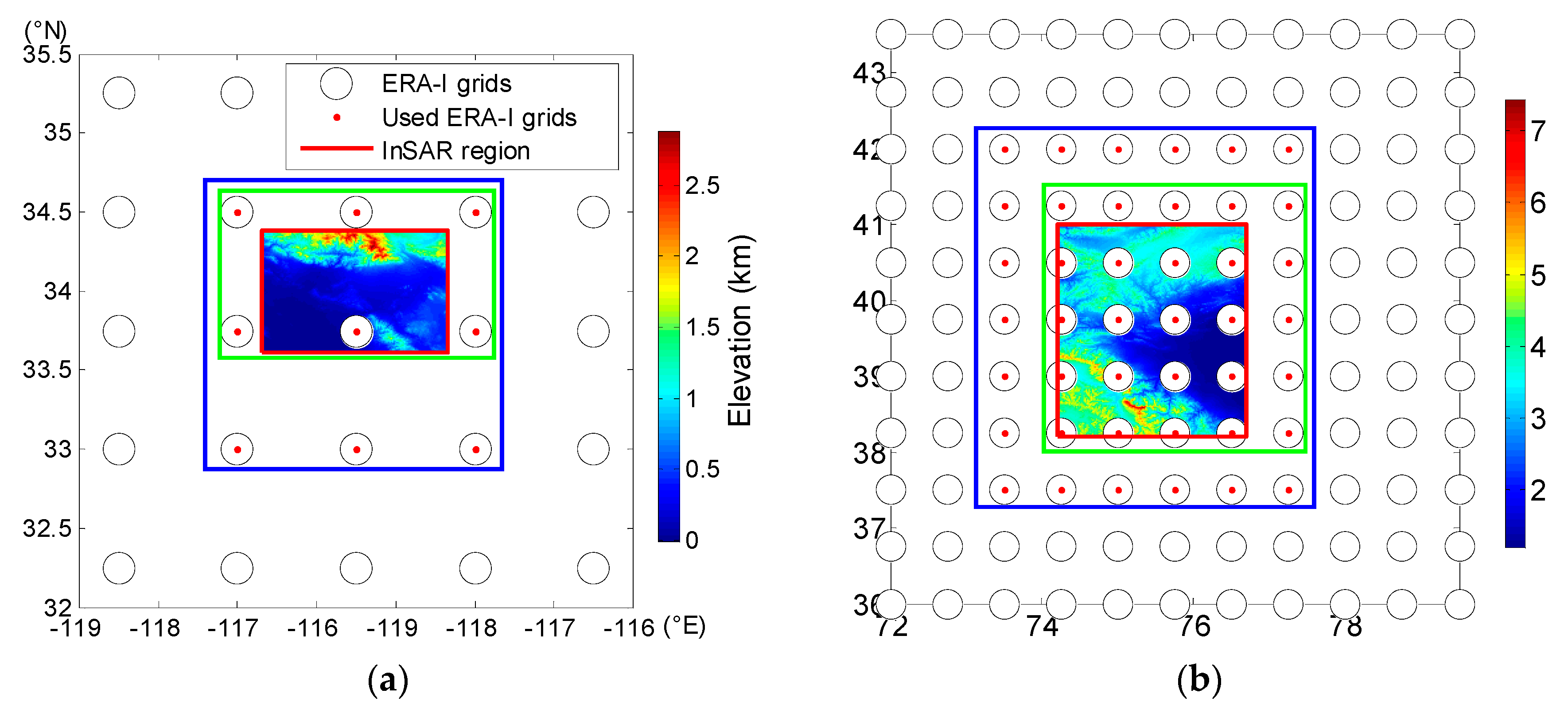
Figure 3.
Mean delay and fitted power law with respect to the elevation. The black solid line represents the corresponding phase delay calculated from the ERA-I data at six grid points (18:00 UTC) on interferogram 20090627/20090905 in California. The points are shown within the green rectangle in Figure 2a. The red dashed line shows the best fit line using the power law model. The black dashed line indicates the maximum height of the InSAR region. (a,b) The tropospheric delays for the master and slave acquisitions show a near power law function with being 1.18 and 1.19. The delay offset at the height of 4.7 km was added back after a log-log linear estimation. (c) The relative tropospheric delay shows a power law relationship relationship ( 1.39).

Figure 4.
Flow chart of tropospheric delay estimation using the PLE method for an interferogram: (1) log-log fitting Equation (8) to obtain and based on ERA-I reanalysis; (2) extracting elevation for all pixels from SRTM DEM; (3) and (4) band filtering in the corresponding spatial wavelength; (5) expanded robust estimation for local (Equation (9)) and (Equation (13)) in each window; (6) local values are extrapolated to each pixel using the multi-weighted method (Equations (14)–(16)); and (7) calculating the final tropospheric delay using Equation (10).
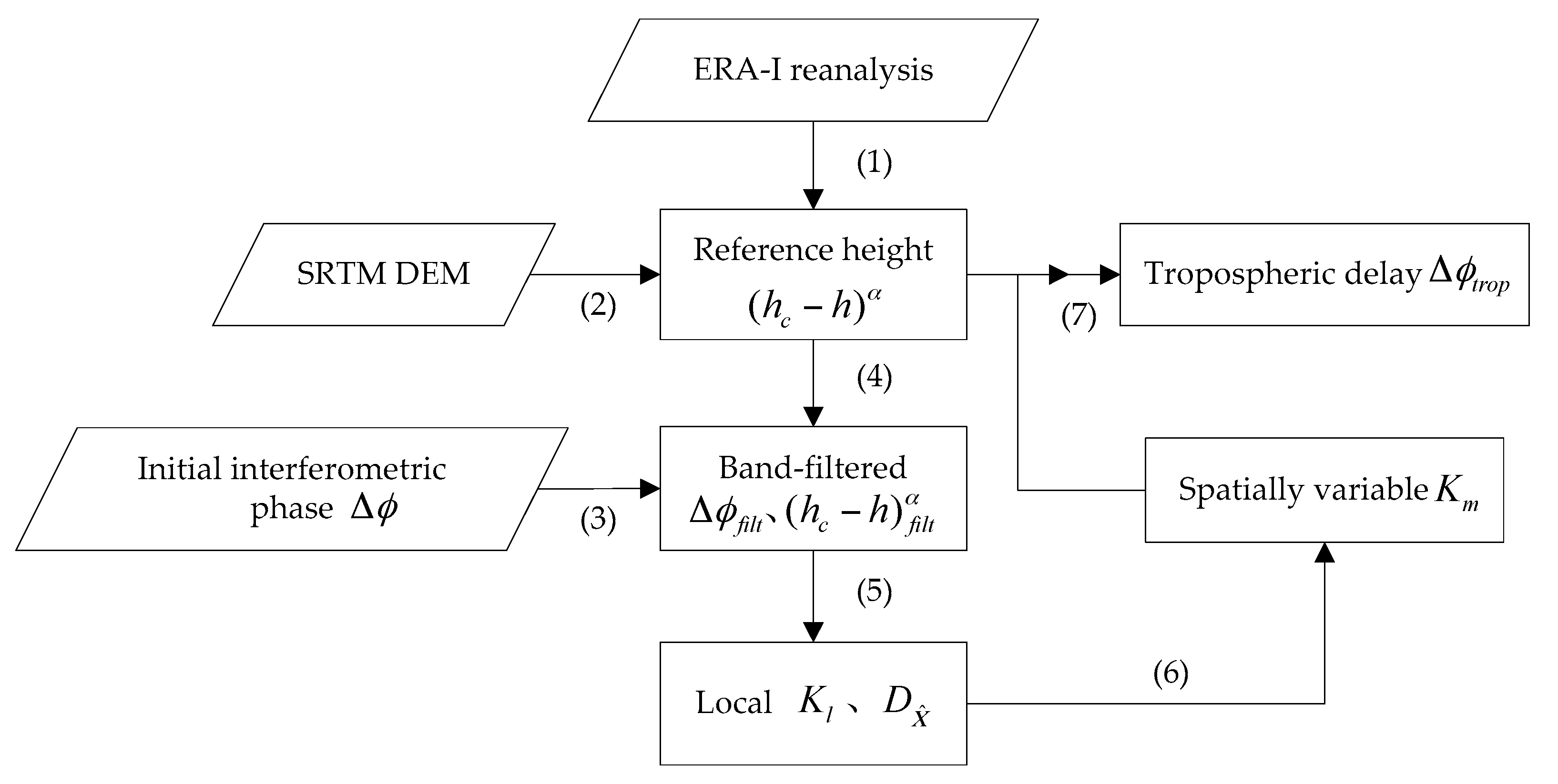
Figure 5.
Comparison of mitigation results of different spatial bands for each interferogram in: (a) California; and (b) Tianshan. The different color bars represent different interferograms. Upper panel represents STD of the unwrapped interferograms (hollow bars) compared to the residual STD after correcting the tropospheric delay derived from the PLE method (filled bars). Lower panel represents reduction of STD after delay correction of different spatial band filters. Arrows were selected for each interferogram to indicate the bands with the largest reduction in STD.


Figure 6.
Examples of constrained height and power law coefficient for our study area in California. Both coefficients were estimated by using ERA-I. We set to the altitude for which the STD and average value of the relative delay offsets are both less than 1.0 rad (~0.45 cm).
Figure 6.
Examples of constrained height and power law coefficient for our study area in California. Both coefficients were estimated by using ERA-I. We set to the altitude for which the STD and average value of the relative delay offsets are both less than 1.0 rad (~0.45 cm).

Figure 7.
Relative tropospheric delays computed from ERA-I reanalysis in California for 120 days (18:00 UTC) between June and October 2009. Relative delay curves are 800 combinations of the tropospheric delay difference at different days, covering the acquisition for interferogram 20090627/20090905 (example in Figure 3). The relative delays did not change significantly at certain height (red arrows) and converged (red lines) at a specific height of 12.8 km. The STD of the relative curves is less than 1 rad. (b) Wet delays converged at the height of 6.8 km. The delays are calculated by integrating the refractivity from surface upward (15 km) and projecting to LOS direction.

Figure 8.
Examples of spatial maps of estimated by the PLE method in California. (a) Interferogram 20080712/20080816. (b) Interferogram 20080816/20081025. (c) Interferogram 20081025/20081129. (d) Interferogram 20100821/20100925.
Figure 8.
Examples of spatial maps of estimated by the PLE method in California. (a) Interferogram 20080712/20080816. (b) Interferogram 20080816/20081025. (c) Interferogram 20081025/20081129. (d) Interferogram 20100821/20100925.

Figure 9.
Examples to test the effectiveness of robust estimation. (a) Outlier rejection results of robust estimation for the original band-filtered data obtained from interferogram 20081025/20081129 in California. (b) Results of robust estimation for the original band-filtered data with extra simulated outliers, which are randomly introduced to the locations. (c) Improvement of STD by robust estimation compared to least squares regression. The average STD improvement (red curve) is calculated from the datasets of 10 simulations. The arrow in (c) indicates the outlier percentage (~22%) with the largest improvement of STD. Gray points in (a) and (b) represent the band-filtered phases, which are considered as “clean observations” without containing outliers. Blue points are suspected to contain outliers (corresponding weights are reduced). Red points are considered to contain outliers (corresponding weights are set to zero), which do not contribute in estimating the scaled factor.
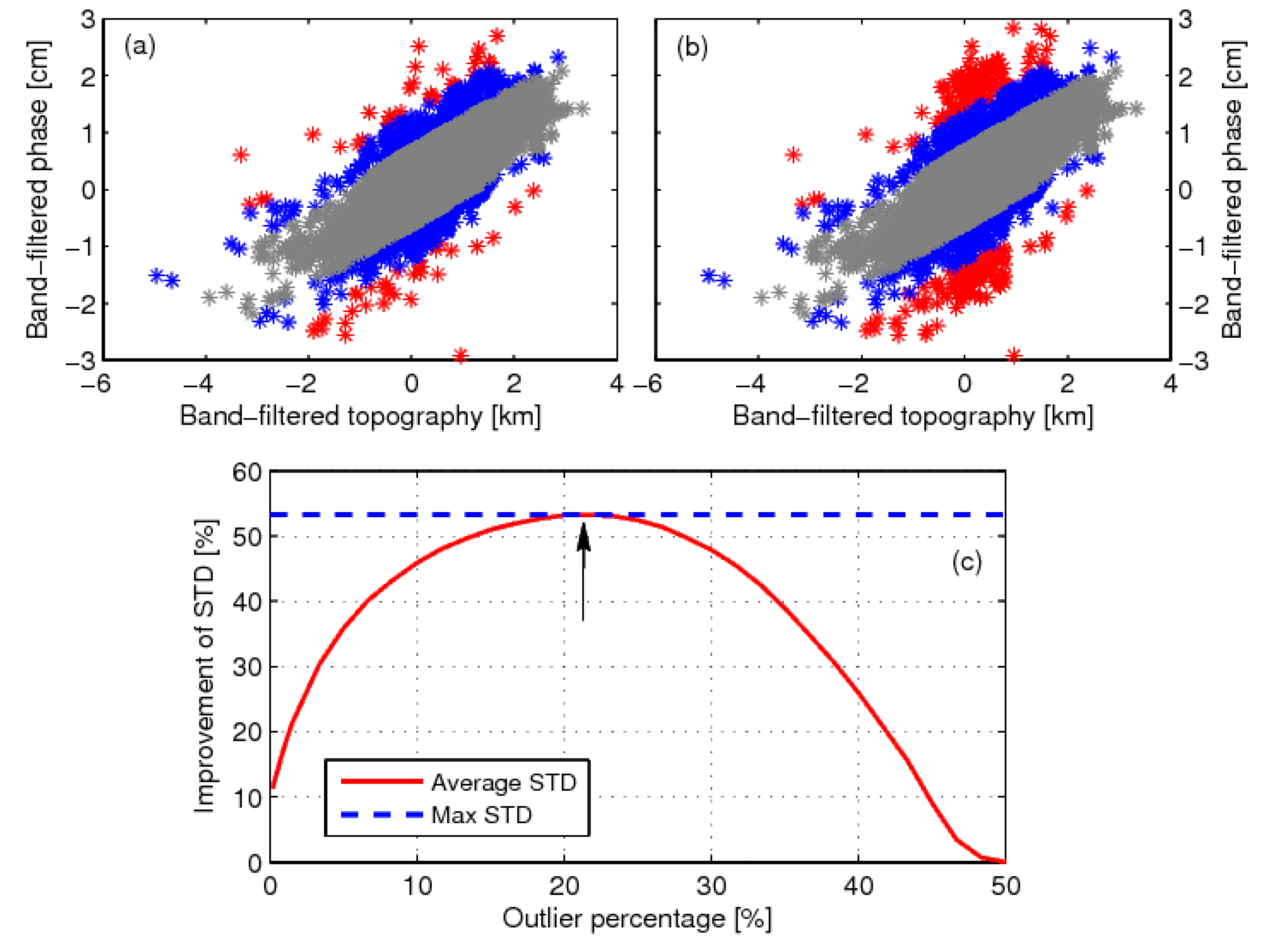
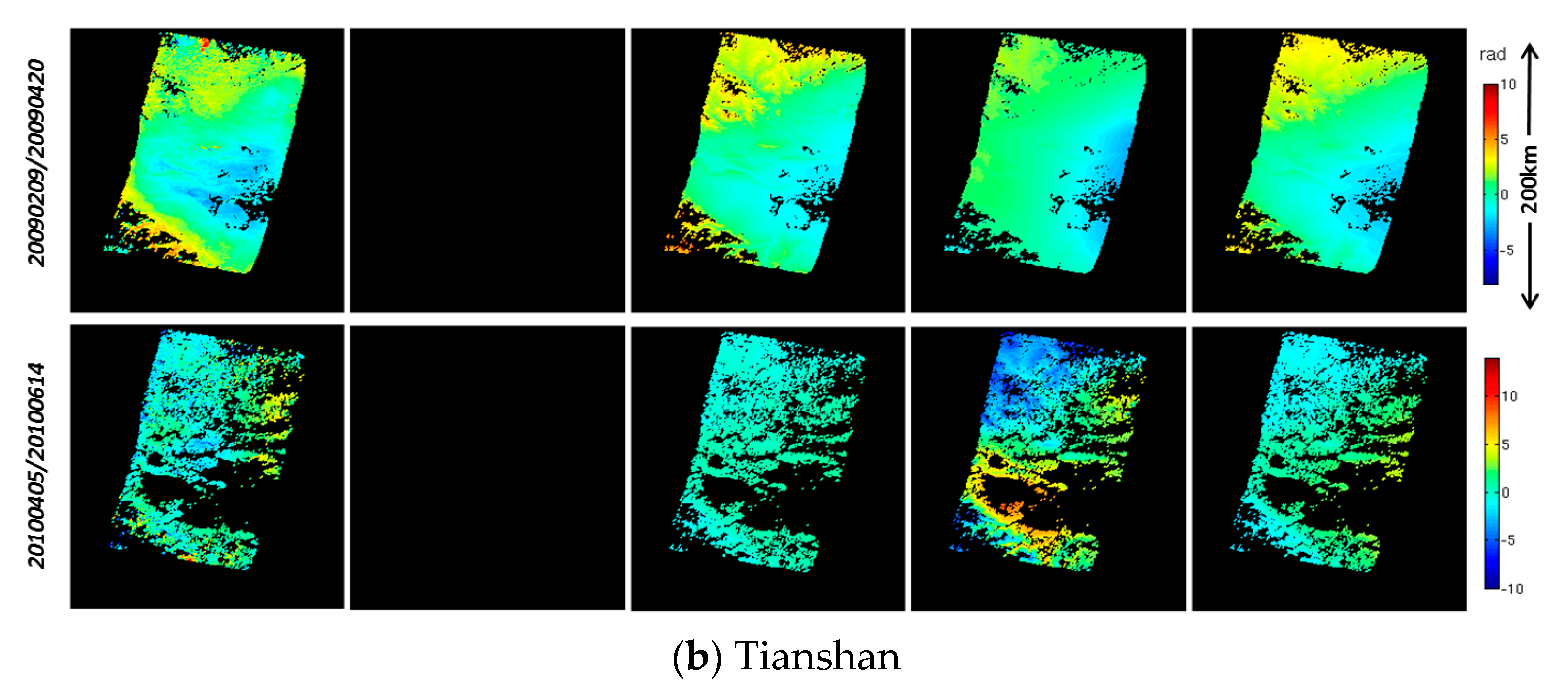
Figure 10.
Examples of tropospheric delay estimated by different methods in: (a) California; and (b) Tianshan. Columns represent the unwrapped interferograms, and the estimated tropospheric delays using MERIS, the linear, ERA-I, and PLE methods (from left to right). All observations are converted to displacements in LOS.


Figure 11.
Relationship between height and hydrostatic delay estimated from ERA-I method in California.
Figure 11.
Relationship between height and hydrostatic delay estimated from ERA-I method in California.
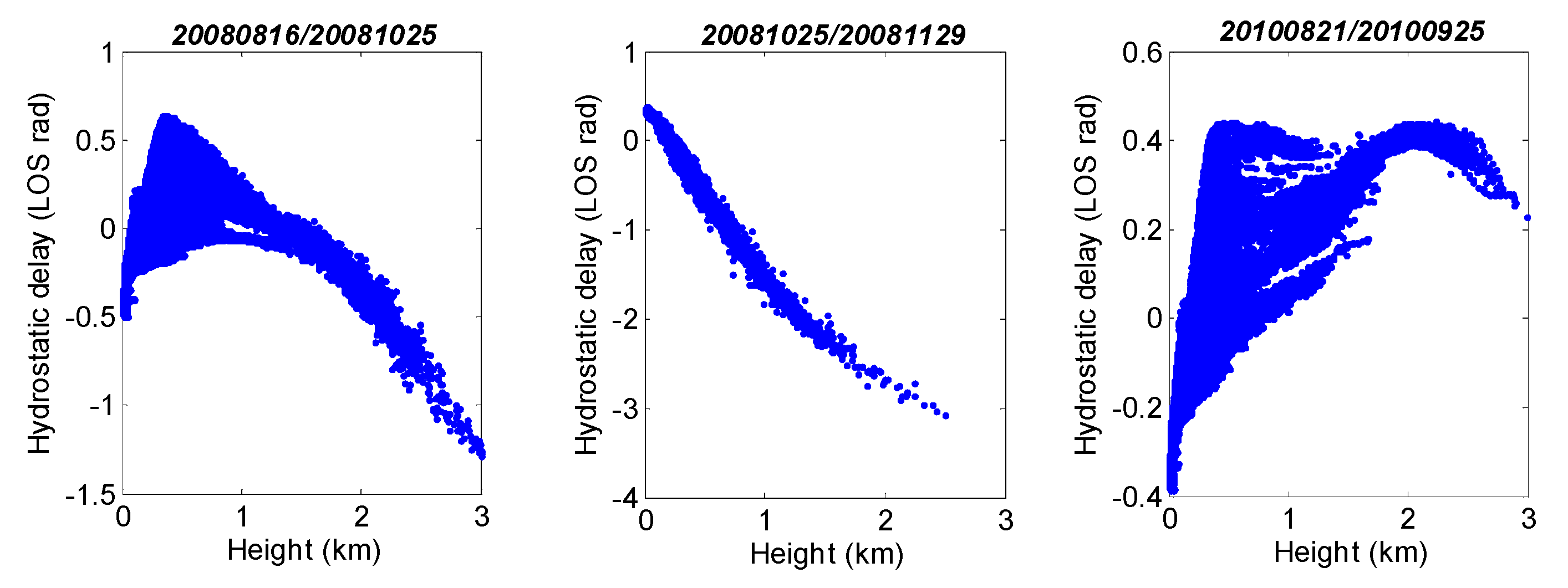
Figure 12.
Examples of final results after different tropospheric corrections in: (a) California; and (b) Tianshan. MERIS delays contain hydrostatic delay component from ERA-I.
Figure 12.
Examples of final results after different tropospheric corrections in: (a) California; and (b) Tianshan. MERIS delays contain hydrostatic delay component from ERA-I.
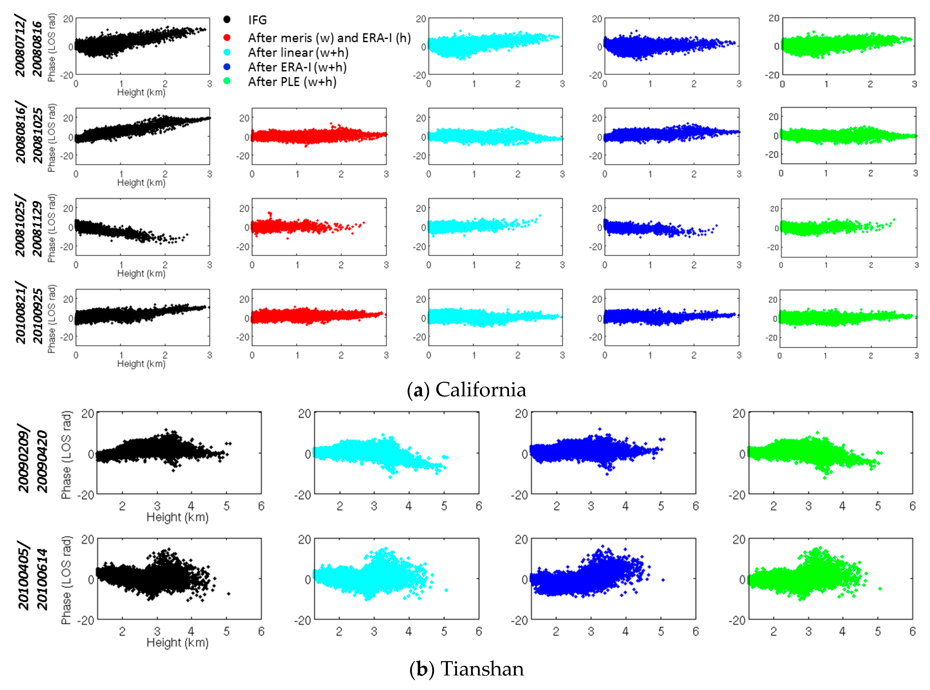
Figure 13.
Comparisons between different tropospheric correction methods in: (a) California; and (b) Tianshan. Left panel: STD of the unwrapped interferograms. Right panel: STD after correction of the tropospheric delay with different methods (colored symbols). Other illustrations show the STD reduction. Point, circle, cross, and square symbols correspond to different interferograms, and triangular symbols represent the average value. Wet delay components are indicated by (w) and hydrostatic delay components by (h).


Table 1.
Parameters of ENVISAT ASAR interferograms.
| California | ||||||
|---|---|---|---|---|---|---|
| Date (yyyymmdd) | Perpendicular Baseline (m) | Temporal Baseline (Days) | Doppler Central Baseline (Hz) | Average Coherence | ||
| 20080712/20080816 | −81 | −35 | −4.0 | 0.28 | ||
| 20080816/20081025 | −13 | −70 | 7.6 | 0.29 | ||
| 20081025/20081129 | −300 | −35 | −8.2 | 0.28 | ||
| 20090627/20090905 | 25 | −70 | 3.0 | 0.30 | ||
| 20100821/20100925 | 343 | −35 | 3.1 | 0.28 | ||
| Tianshan | ||||||
| 20070903/20071112 | −68 | −70 | −4.7 | 0.42 | ||
| 20090209/20090420 | −57 | −70 | 5.8 | 0.41 | ||
| 20100405/20100614 | −153 | −70 | 1.0 | 0.24 | ||
| 20100510/20100614 | 59 | −35 | −4.4 | 0.41 | ||
© 2017 by the authors. Licensee MDPI, Basel, Switzerland. This article is an open access article distributed under the terms and conditions of the Creative Commons Attribution (CC BY) license (http://creativecommons.org/licenses/by/4.0/).
Share and Cite
MDPI and ACS Style
Zhu, B.; Li, J.; Tang, W. Correcting InSAR Topographically Correlated Tropospheric Delays Using a Power Law Model Based on ERA-Interim Reanalysis. Remote Sens. 2017, 9, 765. https://doi.org/10.3390/rs9080765
AMA Style
Zhu B, Li J, Tang W. Correcting InSAR Topographically Correlated Tropospheric Delays Using a Power Law Model Based on ERA-Interim Reanalysis. Remote Sensing. 2017; 9(8):765. https://doi.org/10.3390/rs9080765
Chicago/Turabian StyleZhu, Bangyan, Jiancheng Li, and Wei Tang. 2017. "Correcting InSAR Topographically Correlated Tropospheric Delays Using a Power Law Model Based on ERA-Interim Reanalysis" Remote Sensing 9, no. 8: 765. https://doi.org/10.3390/rs9080765
Note that from the first issue of 2016, this journal uses article numbers instead of page numbers. See further details here.