Wall-to-Wall Tree Type Mapping from Countrywide Airborne Remote Sensing Surveys


1
Department of Landscape Dynamics, Swiss Federal Institute for Forest, Snow and Landscape Research WSL, Zuercherstrasse 111, Birmensdorf 8903, Switzerland
2
Department of Forest Resources and Management, Swiss Federal Institute for Forest, Snow and Landscape Research WSL, Zuercherstrasse 111, Birmensdorf 8903, Switzerland
*
Author to whom correspondence should be addressed.
Remote Sens. 2017, 9(8), 766; https://doi.org/10.3390/rs9080766
Submission received: 14 June 2017
/
Revised: 13 July 2017
/
Accepted: 24 July 2017
/
Published: 27 July 2017
(This article belongs to the Section Forest Remote Sensing)
Abstract
:Although wall-to-wall, accurate, and up-to-date forest composition maps at the stand level are a fundamental input for many applications, ranging from global environmental issues to local forest management planning, countrywide mapping approaches on the tree type level remain rare. This paper presents and validates an innovative remote sensing based approach for a countrywide mapping of broadleaved and coniferous trees in Switzerland with a spatial resolution of 3 m. The classification approach incorporates a random forest classifier, explanatory variables from multispectral aerial imagery and a Digital Terrain Model (DTM) from Airborne Laser Scanning (ALS) data, digitized training polygons and independent validation data from the National Forest Inventory (NFI). The methodological workflow was optimized for an area of 41,285 km2 that is characterized by temperate forests within a complex topography. Whereas high model overall accuracies (0.99) and kappa (0.98) were achieved, the comparison of the tree type map with independent NFI data revealed significant deviations that are related to underestimations of broadleaved trees (median of −3.17%). Constraints of the tree type mapping approach are mostly related to the acquisition date and time of the imagery and the topographic (negative) effects on the prediction. A comparison with the most recent High Resolution Layers (HRL) forest 2012 from the European Environmental Agency revealed that the tree type map is superior regarding spatial resolution, level of detail and accuracy. The high-quality map achieved with the approach presented here is of great value for optimizing forest management and planning activities and is also an important information source for applications outside the forestry sector.
1. Introduction
Precise and regularly updated information on the state, change and distribution of tree types (broadleaved and coniferous tree) is essential for forest related studies, e.g., growing stock estimation [1], biodiversity assessment and monitoring [2], hazard and disease management [3], and sustainable forest management [4]. Forest inventories provide a precise statistical estimation of forest composition for large areas, but spatially explicit information beyond inventory domains is missing [5]. Thus, maps of broadleaved and coniferous trees are an important source of information for assessing woodland resources and an additional valuable output of National Forest Inventories (NFI) [6].
Although the development of remote sensing data sets and methods has opened new perspectives and reached an operational level in the last years, countrywide mapping approaches and sound verification on the tree type level remain rare. In fact, the focus has been placed entirely on either new sensor developments that provide higher spatial, spectral, radiometric and temporal resolution or new image processing and classification approaches [7]. Thus, information on the state and distribution of tree types on a national level has usually been obtained by field inventories [6].
While studies using remote sensing data to map forest composition and tree species reach back several decades, operational countrywide applications have remained uncommon because of economic constraints, as well as low quality imagery, unrepeated flight campaigns and an NFI focus on statistical output and sample-based data collections. Tree species classification approaches based on remote sensing data using the entire line-up of active and passive remote sensing sensors and methods, mostly designed for case studies, range from simple distinction between broadleaved and coniferous trees [8,9,10,11] to identifying main tree species [12,13,14,15]. A comprehensive overview of tree species classification studies is given in the review paper of Fassnacht et al. [7]. In contrast, few studies have covered large geographical extents, e.g., Schumacher and Nord-Larson [16] presented a countrywide wall-to-wall forest attribute map of Denmark, and such studies have been carried out as a side-aspect of other land cover classifications, e.g., the CORINE 2006 land cover (CLC 2006) [17].
Existing maps that principally enable a distinction between broadleaved and coniferous trees are categorical-type maps based on remote sensing techniques and data sets. They have been performed in the framework of global mapping or resource assessment programs and thus vary in legends, spatial resolution (mostly 1 km), temporal coverage, etc. Mentionable are the Global Land Cover (GLC 2000) mapping approach [18], the GlobCover land cover map Version 2 [19], and the MODIS land cover type (MCD12Q1) [20]. Review and uncertainty assessments of these data sets are given in [21]. For Europe, the High Resolution Layers (HRL forest 2012) 20 m forest type map [22] and the European 25 m Forest cover and type map from the Joint Research Center (JRC) [23] are the currently available tree type maps. Finally, Brus et al. [24] presented a 1-km resolution European mapping approach showing the distribution of 20 tree species based on NFI plot data. However, despite the undoubted value of these existing large-scale tree type maps for many applications, unavoidable restrictions due to the coarse spatial resolution and thus the insufficiently detailed representation of tree types (on coniferous and broadleaved level) occur for many forest management demands, especially those at the stand level [7]. Thus, mixed stands in particular are not detected because small-scale information is combined into one pixel. This is an important shortcoming in Switzerland, where mixed stands account for more than 30% of forested area [25].
Although various methods have been developed and used for mapping tree types of forest ecosystems using different remote sensing data, there have been few studies that indicate which method leads to the most accurate models. Remote sensing-based tree species classification has evolved with methodological developments in the domain of statistical learning [7]. Since the mid-1990s, non-parametric decision tree based classifiers, e.g., Random Forest (RF) and Artificial Neural Networks (ANN), have emerged as an alternative to the other classifiers, i.e., unsupervised or parametric methods. Non-parametric methods have the advantage that they do not make assumptions about data distribution, as a normal distribution is not always given [26]. According to Breiman [27] and Hastie et al. [28], RF is one of the most accurate machine learning algorithms. RF is relatively insensitive to the number of input data and the multicollinearity of the data, and it has a smaller prediction variance and therefore usually a better general performance. It runs efficiently on large data sets and may therefore be suitable for countrywide approaches. Moreover, Belgiu and Drăguţ [29] showed in their review paper that the RF classifier outperforms other decision tree classifiers regarding accuracy, training time and stability of the classifier.
New perspectives for countrywide mapping approaches are emerging through digital aerial imagery, which are likely—in contrast to ALS—to be updated more regularly by national mapping agencies [6]. Thus, the possibility of extending the statistical, plot based NFI information to a continuous, landscape level representation has become more feasible. As a part of the Swiss NFI program, wall-to-wall stereo-aerial imagery, provided by the Federal Office of Topography, Swisstopo, on an ongoing cycle with repeated coverage every 6 years, is analyzed [30].
The main objective of the present study was to generate a new high-resolution wall-to-wall tree type map, that consists of the two classes broadleaved and coniferous, for Switzerland. Despite the distinction of only two broad tree type classes, the proposed method is advantageous to other mapping approaches to construct countrywide classification models due to two facts: first, because it uses repeated acquisitions of the same digital aerial imagery and is not the product of different remote sensing data sources, and second, a reliable reference data set exists, which is independent from the training data.
Furthermore, the proposed method was optimized in order to be suitable for European temperate mixed forests within a complex topography. In this paper, we demonstrate a novel approach to deriving a countrywide tree type map with a spatial resolution of 3 m that (i) uses digital aerial imagery and a RF classifier; (ii) is highly automated and reproducible, minimizes computation time, and produces high model and prediction accuracies; and (iii) uses digitized polygons of broadleaved and coniferous trees for model adjustment; and (iv) independent NFI data (aerial photo interpretation) for validation. The tree type map complements the existing spatially explicit countrywide data sets, i.e., the Vegetation Height Model (VHM) [30] and the forest cover map [3] of the Swiss NFI. It is superior to the existing tree type maps regarding level of detail, accuracy and being up-to-date. It also supports forest management demands by providing detailed information on forest composition at the stand level.
2. Materials and Methods
2.1. Overview
To map broadleaved and coniferous trees on a country level, a supervised classification using the RF classifier was applied. Both Airborne Digital Sensor (ADS) images and a DTM from ALS surveys between 2001 and 2015 were used. The ADS imagery was acquired from 2010 to 2015 during the vegetation period, from the beginning of June to the end of August.
To guarantee high computing performance, the whole of Switzerland was divided into 220 equally sized subsets with an extent of 17.5 × 12.0 km, each of which corresponds to one sheet of the national topographic map of Switzerland (scale 1:25,000). Prior to the countrywide mapping, five representative subsets, each within the production regions of the Swiss NFI (see Section 2.2), were used for pretesting. The entire classification approach (computation of the variables, classification and predictions) was done in R 3.3.2 [31]. R reduces the implementation effort and provides many functions that allow parallel clustering that substantially minimized the computation time. The workflow of the countrywide approach is given in Figure 1.
Data preparation involved the orthorectification of the ADS image strips acquired at 0.25- to 0.5-m spatial resolution to obtain a layer stack of the four spectral bands and derived variables at 1-m resolution.
A 3-m regular raster was applied to the layer stack of 1-m pixel size. The resulting raster cells were labeled using the reference data and exploited for training and validation. For the classification approach, mean and standard deviations extracted from the raster cells were used.
Reference data for the forest type classification were acquired in two ways:
- by digitizing polygons of pure broadleaved and coniferous trees on ADS orthoimages
- from NFI plot data based on stereo-image interpretation
The classifications for the 220 subsets were each 10-fold cross-validated five times. The VHM, as described in [30], and a shadow mask were used to mask out non-woodland areas for the final tree type map. The tree type was validated using independent NFI data from stereo-image interpretation.
2.2. Study Area
Switzerland is a central European country on the Alpine arc, located between 5°57′E and 10°29′E and 45°49′N and 47°48′N, and covers an area of 41,285 km2. The country has an altitudinal range between 197 and 4634 m a.s.l. and is characterized by five main types of landscapes: Jura, Central Plateau, Prealps, Alps and Southern Alps (Figure 2). According to Abegg et al. [25]. Switzerland has a varying regional proportion of forest cover with an average coverage of approx. 31%. Broadleaved trees make up 47.1% and coniferous trees 52.9% of the forest species composition. Species richness is higher in the Central Plateau than in the mountainous regions. Forests in the Central Plateau up to approx. 1200 m a.s.l. are managed to a high degree and are dominated by beech (Fagus sylvatica), ash (Fraxinus excelsior), oak (Quercus sp.), white fir (Abies alba), and spruce (Picea abies). The dominant tree species are Scots pine (Pinus sylvestris), larch (Larix decidua), and spruce (Picea abies), in addition to the typical broadleaved and softwood species growing along rivers and streams. The upper tree line varies between 1600 m a.s.l. in the northern Prealps to an average of 2300 m a.s.l. in the valleys of the Central Alps, and is often dominated by larch, Scots pine, and shrub forests with creeping pine (Pinus mugo) and green alder (Alnus viridis). More detailed information on Swiss forests is provided in the third NFI report [32].
2.3. Remote Sensing Data
The tree type mapping approach is based on three countrywide data sets. First, ADS40 and ADS80 imagery (described in detail in Waser [33]) was used, with images acquired by Swisstopo in June, July and August from 2010 to 2015. Swisstopo imagery follows a 6-year leaf-on cycle for the whole country. Images were acquired strip-wise East–West by two Charge-Coupled Device (CCD) line-scanners, at four bands of true color and near-infrared (RGBI), with a 12-bit radiometric resolution and Ground Sample Distances (GSD) of 25–50 cm (Table 1). Since both topographic and radiometric corrections (ATCOR 3) caused severe artifacts in the imagery, the original images were used. In total, from the 1710 stereo-image strips with a total length of 62,000 km covering a countrywide RGBI, an orthoimage mosaic with a spatial resolution of 1 × 1 m was generated. The orthorectification was done with SocetSet 5.6 (BAE Systems) and the mosaicking was done with OrthoVista7.0 (Trimble).
Second, the DTM swissALTI3D from Swisstopo, which is based on ALS data (<2000 m a.s.l.) and image matching (>2000 m a.s.l.), was used to derive topographic variables. The ALS data were acquired between 2001 and 2015 with an overall point density of 0.5/m2. The original swissALTI3D has a spatial resolution of 2 m, and it was resampled to 1 m [34]. Third, a VHM was produced following methods described in [30]: A Digital Surface Model (DSM) with a spatial resolution of 1 m was calculated using the same imagery described above. It was then normalized to obtain the actual vegetation heights using the DTM swissAlti3D. The buildings were masked out using the building footprints from the Topographic Landscape Model of Swisstopo and the spectral information of the image data.
2.4. Reference Data
2.4.1. Digitized Polygons
The collection of reference data for the two tree types, broadleaved and coniferous, is based on delineations on the RGBI orthoimage mosaic and was done individually for each of the 220 subsets. To facilitate the collection of homogenously distributed training samples, each subset was divided into 16 equally sized squares for which the reference polygons were digitized within the forest patches and outside of shadows to reduce the within-class variance of the two tree types. In order to have an objective and representative training sample, an area-proportional and class-balanced allocation was used. This implies also the size of the polygons, i.e., typical large canopy trees, groups of crowns within pure stands but also single tree crowns within a stand of the other class. An optimal distinction between broadleaved and coniferous trees was obtained by switching between the RGB and CIR image bands during the delineation. Thus, it was possible to achieve a large sample with a very high certainty for the chosen reference polygons. In total, 185,240 polygons were digitized by experienced interpreters using standard GIS software. Table 2 summarizes the main attributes of the reference sample.
2.4.2. NFI Data
Swiss NFI data were used as an independent data set to validate the tree type map. The Swiss NFI is a continuous survey with plots surveyed over a period of nine years following a two-phase sampling approach that incorporates terrestrial surveys and aerial stereo-image interpretation. Stereo-image interpretation is conducted yearly over an area of 50 × 50 m around the plot center for one-ninth of the NFI sample plots on a 1.4 × 1.4 km grid covering the entire area of Switzerland using ADS stereo-imagery from 2006 to 2016. Each interpretation area (IA) consists of 25 equally spaced (10 m) lattice points (sub-sampling points) arranged in a 5 × 5 point design. See Figure 3 and Mathys et al. [35] for details. At each lattice point, the elevation is measured and 11 land cover classes are interpreted. From these classes, coniferous trees (including larch, a deciduous conifer) and broadleaved trees were used as a reference and their proportion was calculated per interpretation area. In sum, 4191 IAs that are entirely or partly located within the tree type map were surveyed.
2.5. Variable Computation
Besides using the original image bands, RGBI-related explanatory variables were included based on studies about image processing [36,37]. The four image bands (Table 1) were used as the basic spectral variables. Additionally, based on the tree species classification described in [12,33], the bands RGB and NIR from the original ADS80 were color-transformed into intensity (I), hue (H), and saturation (S), to separate the effect of illumination from the quantity of intensity. These three new variables are: I[RGNIR], H[RGNIR], and S[RGNIR], as designated in [7,38]. Remote Sensing Indices (RSI) have been extensively used to explore vegetation’s spectral signature characteristics, i.e., tree species classification, both in the visible and near-infrared part of the spectrum [39]. In the present study, the Modified Soil-Adjusted Vegetation Index (MSAVI2) [40] (Equation (1)) was additionally computed.
Thus, eight variables were computed from the image bands (four original image bands and four derived variables). Additionally, the two topographic variables elevation (above sea level), and aspect (compass direction that a topographic slope faces, i.e., terrain exposition) were derived from the DTM swissALTI3D. Both elevation and aspect are determinants of the biological and physical characteristics of vegetation communities, such as tree types, soil moisture and evapotranspiration [41]. In sum, ten variables were computed from the remote sensing data sets and a layer stack was generated.
2.6. Classification
2.6.1. Pretesting
Since the generated layer stack of 1-m pixel size is an enormous amount of data and would make a highly automated countrywide tree type classification approach less feasible, a coarser classification unit was chosen. Based on the findings from previous tree species classification studies, which were based on the same image data and tested with a spatial resolution between 1 m [12] and 5 m [33,42], a countrywide 3-m regular raster seems to be adequate, regarding both level of detail and computation time. Thus, each raster cell consists of nine pixels from each of the ten variables. For each raster cell, the mean and standard deviation of each of the ten variables were computed for the classification. The resulting raster cells were labeled using the reference data and exploited for training and validation. The 3 × 3 m regular raster cells were sometimes mixed with digitized polygons and non-tree objects. Since including such raster cells would bias the mean and standard deviation of the variables computed for each raster cell, these cells were disregarded during the computation of mean and standard deviation values. Large shadowed areas were separated using intensity values I[RGB] from the IHS-transformation of the RGBNIR bands, where values smaller than 0.02 were assigned to shadows—as tested by Waser [33] for tree species classifications using the same imagery. The threshold was determined by first checking the histogram of the intensity orthoimage and, based on visual inspection, separating shadowed and non-shadowed areas. Pixels belonging to this shadow mask were excluded from the final tree type map.
In order to find the most appropriate classification approach regarding processing time and accuracy of both the models and the predictions, five of the 220 subsets were selected, which are representative of the entire area regarding topography, landscape (Jura, Central Plateau, Prealps, Alps and Southern Alps), and tree species composition. Based on case studies [12,33,42] that used tree species classification and ADS80 imagery in Switzerland, three classifiers, Logistic Regression Model (LRM), Support Vector Machine (SVM) and Random Forest (RF), were preliminarily tested. Whereas all classifiers produced high accuracies that were not significantly different from each other—with the exception of SVM—the variability in processing time was high and RF clearly performed best (see Table 3 and Table 4).
2.6.2. Random Forest Classification
For each of the 220 subsets, a RF classification was performed as described in detail in Breiman [27]. Random Forest is a widely used ensemble classifier that produces multiple decision trees, using a randomly selected subset of training samples and variables. It consists of many decision trees (individual learners that are combined) and outputs the class that is the mode of the class’s output by individual trees. It uses bootstrap aggregating, i.e., bagging, to create different training subsets to produce a diversity of trees, each providing a classification result for the samples not chosen. The output class is obtained as the majority vote of the outputs of a large number of individual trees. Moreover, computational efficiency of the algorithm is enhanced, compared with alternative approaches, as only a sample of variables is used at each node split [43].
RF is also relatively insensitive to the number of input data and multicollinearity of the data, and it has a smaller prediction variance and therefore usually a better general performance [28]. RF generates an internal unbiased estimate of the generalization error, using samples that are excluded from the training subset (so-called “out-of-bag” (OOB) samples). Moreover, RF provides a measure of the input features’ importance (Mean Decrease in Accuracy (MDA)), through random permutation, which can be used for feature ranking or selection [44].
In this study, the RF implementation randomForest in R 3.3.2 [31] was used. A RF model consists of two parameters (1) number of trees to be grown in the run (ntree) and (2) number of features used in each split (mtry). According to other studies [15,29,45,46], the default values (ntree set at 500 trees and mtry set equal to the square root of the total number of input features) often provide satisfactory results. For the final tree type map, the single predictions of the 220 subsets were merged into one data set. All pixels of the countrywide available VHM lower than 3 m according to the Swiss NFI definition [32] were then masked out. The VHM is based on the same imagery that is used for the tree type mapping.
2.7. Accuracy Assessment
2.7.1. Model Accuracies
The Random Forest classification was applied to each of the 220 subsets, and the predictive power for broadleaved and coniferous tree type models was verified by 10-fold cross-validation repeated five times. A value of ten for k-fold cross-validation is frequently used for estimating the generalization error [47]. In doing so, the reference polygons in each subset are randomly split into ten subsets of the overall data set, each including around 10% of the samples of the two classes, broadleaved and coniferous. In each training step, an RF model was trained with 90% of the reference samples and applied to the remaining 10% (i.e., the validation polygons). This step was repeated ten times, and the ten results were aggregated to one confusion matrix. The overall accuracy (OA), Cohens kappa coefficient (K), commission errors and omission errors were calculated based on the error matrix for accuracy assessment. For details see Richter et al. [48].
2.7.2. Map Accuracy
The validation of the tree type map was performed using the 4191 interpretation areas (IAs) of the NFI for which the fraction of broadleaved and coniferous trees was computed. To fit the 50 × 50 m area of the IA, the tree type map was resampled to 1 m. In a first step, for each IA, differences between the predicted (tree type map) and observed (NFI image interpretation) broadleaved fraction were calculated. In a second step, the influence of the following parameters: NFI production regions, NFI elevation levels, terrain exposition, percentage of conifers, location at forest edge, presence of other land cover classes, and time lag, i.e., time difference between the imagery used for the stereo-interpretation and the imagery used for the tree type map, on the accuracy of the prediction was statistically tested using multiple linear regression [49]. Additionally, the parameter ‘number of lattice points falling on trees’ per IA (ranging from 1 to 25) was determined and used as predictor as well because this parameter may affect the validation result. Thus, the minimum number of points per IA that is required for this parameter to have no significant influence on the validation result was determined using a stepwise procedure. Finally, the total number of IAs was reduced to 3373 (only the IAs with nine or more lattice points falling on trees were included). The output of the final model is given in table in Section 4.2. For these IAs the following statistical accuracy measures were calculated: Median (M), absolute Median (Mabs), Normalized Median Absolute Deviation (NMAD), and Root Mean Squared Error (RMSE). M, Mabs and NMAD are robust accuracy measures as a way to deal with non-normal data distributions [50]. The Mabs was calculated as the median of absolute differences between predicted and observed broadleaved fractions in the IAs (Equation (2)).
where denotes the difference between the predicted and observed broadleaved fraction in the ith IA.
The NMAD is the normalized median of the absolute deviations from tree type map and IAs differences’ AI median. NMAD can be considered as a measure of statistical dispersion, but it is more resilient to outliers in a data set than the standard deviation [50]. The calculation of NMAD is given in Equation (3):
The calculation for RMSE is given in Equation 4:
where is the difference between the predicted and observed broadleaved fraction in the ith IA, is the mean of differences in all IAs, and n is the total number of IAs.
3. Results
3.1. Model Accuracies
For the 220 subsets, the average model overall accuracy (OA) was 0.99 (ranging from 0.95 to 0.99) and Kappa averaged 0.98 (ranging from 0.83 to 0.99), with some variation in the NFI production regions. Figure 4 shows that the highest variation occurs for the NFI production region of the Alps. For 5% of the subsets, the overall accuracy was lower than 0.98, whereas it was higher than 0.99 for 50% of the subsets.
3.2. Tree Type Map
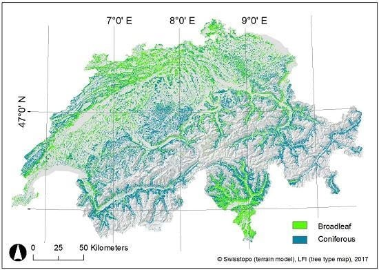
The result of the RF-based tree type mapping of the 220 subsets is presented in Figure 5 as an aggregated wall-to-wall tree type map for all of Switzerland with a spatial resolution of 3 m. The map clearly shows that conifers are the dominant tree type in the higher elevation areas (Jura, Prealps, Alps) and broadleaved trees generally dominate in the lower regions, in lower valleys of the Prealps and Alps, and in the southern parts of Switzerland.
The accuracy assessment of the tree type map (Section 3.3) was performed using independent NFI data. Additionally, it was aggregated and compared to the most recent and existing High Resolution Layers (HRL forest 2012) forest type map with a spatial resolution of 20 m [22] (see Table A1). The final tree type map was visually checked, in particular regarding border effects between neighboring image strips and between adjacent subsets. No systematic errors or abrupt changes in the tree type mapping were detected during this inspection.
3.3. Indpendent Validation
During independent validation, the predicted (tree type map) and observed (NFI image interpretation) broadleaved fractions in the IAs were compared. The validation was performed for 3373 IAs, for which at least nine lattice points fell on trees (see Section 2.7.2). The effects of the parameters NFI production regions, NFI elevation levels, terrain exposition, stand composition (percentage of conifers), location at forest edge, presence of other land cover classes within the IA, and time lag of the imagery on the accuracy of the tree type map were analyzed (see Table 5).
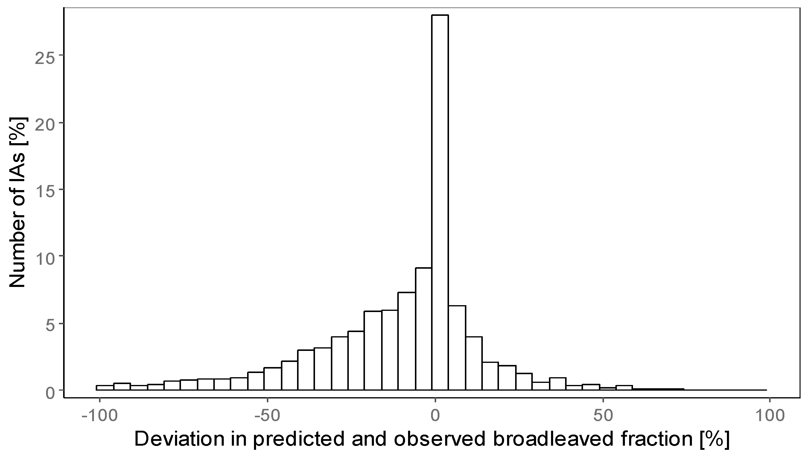
The distribution of the deviations between predicted and observed broadleaved fractions in the 3373 IAs is illustrated in Figure 6.
In Figure 7, the smallest deviations (±10%) in the fraction of broadleaved trees between the two data sets are depicted in green. These are regions in the Alps with a few outliers (red represents overestimation of broadleaved, and blue represents overestimation of conifers) in the valleys. The largest (negative) deviations in the broadleaved fraction indicate an overestimation of conifers (blue), which is concentrated in three regions: the east part of Switzerland, the central part and the Southern Alps.
Table 5 shows the overall agreement in the broadleaved fraction between NFI data and the tree type map. The negative value of the median (−3.17%) indicates a general underestimation of the broadleaved fraction in the tree type map. The Mabs indicates that, for 50% of the IAs, the difference between predicted and observed broadleaved fractions was smaller than 9.75%. Furthermore, the analysis resulted in an NMAD of 13.82% for all IAs and an RMSE of 26.51%.
More detailed analysis revealed that the smallest disagreements in the broadleaved fraction between the tree type map and the NFI IAs occurred in the Alps and in areas higher than 1401 m a.s.l. Whereas conifers are the dominant tree type in these areas, pure stands with a dominance of coniferous tree species (>91%) also occur in all other regions. The largest disagreements occurred in the Prealps, the Central Plateau and the Jura and in areas below 1400 m a.s.l. These areas are dominated by pure broadleaved and mixed stands. Furthermore, terrain exposition also affects the accuracy, and disagreement between the two data sets was highest for areas with a west to north exposition. Finally, the validation revealed that the location of the IAs in terms of forest edge had an influence, with differences clearly larger at the forest edge.
4. Discussion
4.1. General Aspects of the Tree Type Mapping Approach
From a methodological point of view, the presented approach is appropriate for wall-to-wall mapping of entire countries. It is flexible regarding the kind of input data sets that are routinely acquired during the vegetation season over a time span of a few years, and it can process such data sets in a reasonable computation time. The generation of training samples for the tree type map was a time intensive and—to a certain degree—subjective task in the entire methodological workflow. At first glance, the large number of over 185,000 digitized training polygons might seem to be overdrawn, but it was required for obtaining representative samples for imagery from different acquisition times and years and was necessary because NFI data were only used as an independent data set for validation. Due to the sensitivity of RF classification to the sampling design and imbalanced training samples [51,52], the training samples for the tree type map had to be balanced and representative of the two classes, i.e., area-proportional, and large enough to accommodate the large number of data dimensions. In fact, reducing the number of samples to a certain degree would only slightly lower the model accuracies [7] but would have a greater (negative) impact on the prediction of the tree types. To the best of our knowledge, no other countrywide approaches exist that have used additional independent data to validate the predictions. For example, NFI plot data were used as training and validation data to predict forest resources in combination with ALS data [16] and with satellite imagery [53]. Although the collection of sufficient training data was a time consuming part of the process, the tree type mapping approach as a whole remains highly automated due to two facts.
First, pretesting was applied to five representative areas in order to determine the exploratory variables that contributed most (thereby reducing the large amount of data) and to assess the most appropriate classification algorithm. Compared with LRM and SVM, the RF classifier clearly performed best regarding computation time but did not result in significantly higher model accuracies. This finding is in accordance with results from other related studies [7,15,26].
Second, computing tree type was facilitated by splitting the entire area into 220 subsets. Remarkably, the aggregation of the predictions of the subsets to the connected tree type map produced no serious border effects or abrupt changes of the tree types within the forest stands, indicating that the modelling approach was robust. It seems that these effects usually increased when neighboring images were acquired on different dates (see Section 4.4).
The computation of explanatory variables was based on previous case studies [12,33] that dealt with tree species classification using the same countrywide image and ALS data. In accordance with these studies, the simple usage of the four original image bands, the band ratios, and the index MSAVI enabled us to classify tree types with high accuracy. The topographic variables aspect and elevation were further used to reduce the effects of relief shadows and large elevation differences in the terrain (see Section 4.4). Furthermore, first feedback from users of the tree type map, i.e., foresters, environmental agencies and governmental authorities, are positive and reveal that the spatial resolution and level of detail are sufficient. Thus, we believe that the tree type map approach provides an optimal balance between a sufficient level of detail and reasonable computation time. In their review paper, [7] reported that a successful species classification is not solely based on a high spatial resolution but depends on other factors, e.g., spectral resolution, the availability of representative reference data and the mission behind it, i.e., the end user.
4.2. Tree Type Map Compared with NFI Data
Although the classification models yielded a high level of precision across the entire data set, predicted values were generally positively biased compared with NFI data for coniferous and negatively biased for broadleaves trees. However, NFI interpretation is an independent data set for comparisons rather than the truth, and therefore the absolute deviations must be carefully interpreted. Moreover, due to the fact that estimation accuracies for broadleaved and coniferous fractions by terrestrial field surveys are in the range of 10% [54], the obtained differences between predicted and observed broadleaved fractions of less than 10% can be interpreted as reasonable (50.6% of IAs). Table 5 reveals that underestimation of the broadleaved fraction mainly occurs in mixed forests in all parts of the country, with a higher concentration in the Central Plateau, the Jura and the Prealps. It increases with decreasing elevation and is therefore more distinctive for broadleaved stands—especially in areas with west and north terrain expositions. Broadleaved trees are dominant in regions below approx. 1000 m a.s.l., and coniferous trees are dominant above this elevation. Applying multiple linear regression revealed that production region, terrain exposition, elevation a.s.l., percentage of coniferous trees, presence of other land cover classes and time lag of the imagery used for the NFI data and the tree type map have a significant influence on the agreement between the predicted (tree type map) and observed (NFI image interpretation) broadleaved fraction in the IAs (Table 6). The reasons for the deviations are manifold and can be separated by these parameters.
First, the parameter production region had a significant effect on the agreement of broadleaved fractions between the tree type map and the NFI data. In the Prealps and Alps, the agreements differed from the Jura at the 0.001 significance level, whereas the Central Plateau and Southern Alps differed from the Jura at the 0.05 significance level.
Second, terrain exposition was a key factor contributing to the overestimation of conifers on northern slopes. This effect increased in alpine regions but also occurred in the hilly regions of the Central Plateau. Moreover, Table 6 reveals that the agreement between the two data sets was significantly higher for slopes with east, south and west expositions. Terrain exposition clearly affected the spectral properties of the broadleaved trees in particular (see Section 4.4). The sun-sensor geometries were responsible for shadows in the northern and particularly western expositions and affected the tree type mapping.
Third, elevation had a significant influence on the agreement between the two data sets. The deviations decreased significantly with increasing elevation, which meant a decrease in the fraction of broadleaved trees.
Fourth, a decrease in the fraction of coniferous trees had a significant impact on the agreement between the two data sets. The highest deviations occurred for mixed stands with a proportion of conifers between 11% and 50%, and there was a slight decrease in deviation for pure broadleaved stands. Thus, to a certain degree, the fewer coniferous trees present, the higher the deviations. This is in accordance with the parameter elevation. Moreover, visual inspection revealed that this effect decreased for young or very closed broadleaved stands because shorter trees and denser crowns have smaller cast shadows and shadows within crowns.
Fifth, analogous to the forest mask [3], it was expected that forest edge might have an impact on the agreement between the two data sets. Although Table 5 indicates that deviations between the two data sets were greater at the forest edge than within the forest, Table 6 shows that the location of the IAs had no significant influence. This was also caused by removing the IAs with fewer than nine points interpreted as trees (which is often the case for IAs at the forest edge) during the stepwise fitting of multiple linear regression. Moreover, visual inspection of the tree type map revealed that the shape of extracted tree patches, e.g., linear tree cover elements, groups of trees and single trees in orchards or urban areas, affected the classification more than proximity to the forest edge. As trees located at the forest edge were often misclassified as conifers, this is a particular weakness of the countrywide data set.
Sixth, Table 6 reveals that the presence of other land cover classes (e.g., shrubs, grass, bare soil) had a significant influence on the agreement between the two data sets. Whereas the photogrammetric experts most likely interpret these classes correctly using the stereo-images, even in the shadowed parts, they were neglected by the classification approach and were classified as coniferous trees.
Seventh, a time lag between the imagery used for the stereo-interpretation and the imagery used for the tree type map equal or greater than 6 years had a significant influence on the agreement between the two data sets. The greater the time lag between the two images, the more likely the proportion of broadleaved and coniferous trees within the IAs has changed (forest management, storm event).
Finally, slight differences between the two data sets might have resulted from the tree cover mask, which was based on the countrywide vegetation height model. According to Ginzler and Hobi [30], VHM is less accurate and more error-prone in areas with shadows for which image-matching is particularly challenging.
4.3. Map Quality Compared to Pre-Existing Maps
In principle, a comparison of the tree type map with pre-existing maps is informative and helpful for interpreting differences between the data sets. However, the existing global data sets are too coarse, with a spatial resolution of 0.5–1 km, and outdated. Furthermore, comparisons with the only and latest official available tree type map of Switzerland (WMG25) provided by the Federal Statistical Office [55], and also with the European 25 m resolution forest cover and type map from the Joint Research Center (JRC) [23], were regarded as inappropriate because substantial changes in the forest composition likely occurred since these maps were produced more than 10 years in advance [25]. Thus, the most appropriate remaining data set is the High Resolution Layers (HRL forest 2012) 20-m resolution forest type map [22], which is the most recent available and detailed map of Switzerland.
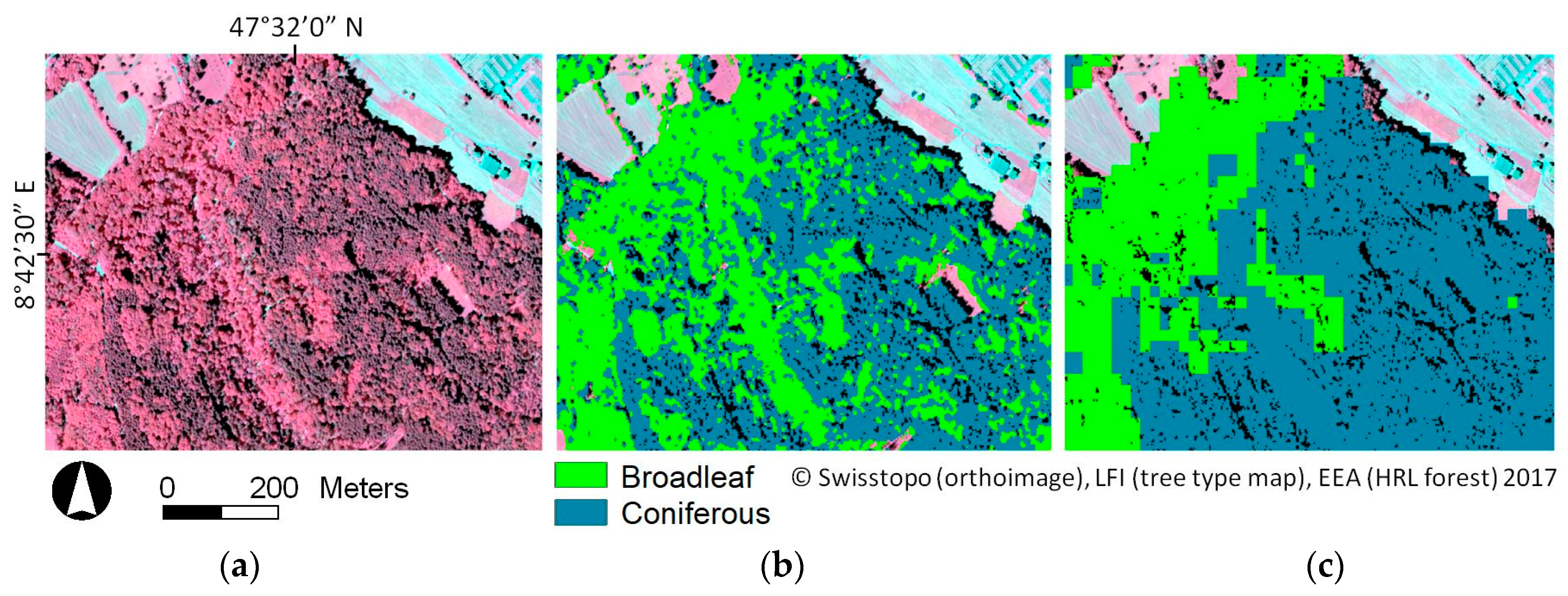
Similar to the tree type map, HRL forest 2012 was compared with the IAs and the deviations in broadleaved fraction was assessed. The validation was performed for 3210 IAs (163 fewer IAs than for the tree type map due to the different extent of the data sets) that had at least nine points interpreted as trees. For details on the numbers see Table A1 (Appendix). The comparison revealed that this map deviated more from the IAs than the tree type map (e.g., RMSE 34.8% versus 26.5%), but the overestimation and underestimation of broadleaved fractions was more even over the entire country (median 0% versus −3.2%). However, the large difference in spatial resolution between the tree type map (3 m) and the HRL forest 2012 forest type map relativizes the absolute numbers obtained by the comparisons. Although this might suggest a roughly comparable spatial distribution of the tree types from the tree type map and the HRL forest 2012 forest type map, Figure 8 clearly shows that this was not the case. The differences are more likely due to misclassifications of the Landsat imagery and the coarser spatial resolution than the time gap of a few years between the two data sets. Change in forest composition is a relatively slow process over many years, with the exception of clear cutting or storm events.
Furthermore, Table A1 (conifers in %) reveals that the purer a stand is—broadleaved or coniferous—the smaller the differences between the NFI data and the HRL forest 2012 layer. In contrast to the tree type map, deviations increased in regions between 600 m and 1400 m a.s.l., which are clearly dominated by mixed stands. This is a particular drawback of the HRL forest 2012 forest type map because Switzerland is dominated by mixed stands over large areas (Central Plateau, Jura, Prealps). Thus, the HRL forest 2012 forest type map might be more appropriate in boreal forests or in forests with pure stands. The HRL forest 2012 forest type map also seems to be less sensitive than the tree type map to the parameter location and presence of other land cover classes. Slightly higher deviations between NFI data and the HRL forest 2012 forest type map (compared with the tree type map) were obtained for north-oriented areas, most likely due to image-related constraints, i.e., illumination and acquisition date and time, similar to those of the tree type map.
4.4. Constraints of the Tree Type Mapping Approach
Sources of error in the tree type map are manifold and are related more to the input image data and less to the proposed classification approach. As expected, date and time of data acquisition influenced phenology and illumination of the images, which led to high spectral variability, and thus had a large impact on the resulting tree type map, in particular regarding broadleaved trees. The few image strips acquired in early June were not optimal for mountainous regions. Whereas trees in the valleys already had unfolded leaves, foliage was still missing in higher areas. Thus, for classifying tree types in the Central European Alps, image acquisition should be limited to from the end of June to the end of August and preferably completed around noon to provide a large zenith angle of the sun. Besides the phenological aspects, the negative impact of illumination effects, such as cast shadows or shadows within crowns, could be minimized in this way. However, the present study had to cope with two restrictions: first, the imagery was acquired on an operational basis by the national mapping agency in an ongoing cycle and therefore not on request with individual user specifications. Second, topographic and radiometric corrections, often suggested in the literature [56], caused severe artifacts, i.e., blurred areas, over large areas and also in areas, i.e., flat terrain, that were less affected by the topography. Assuming that topography in particular might affect illumination and spectral separability of broadleaved and coniferous trees, two RF classifications for a subset of approx. 200 km2 were performed, one based on the original RGBI imagery and the other based on the ATCOR3 [57] corrected imagery. The tests revealed that these artifacts affected the classification and resulted in lower overall accuracies (OA 0.982 for the original imagery, 0.941 for the corrected imagery (based on 840 digitized polygons, 10-fold cross-validated)).
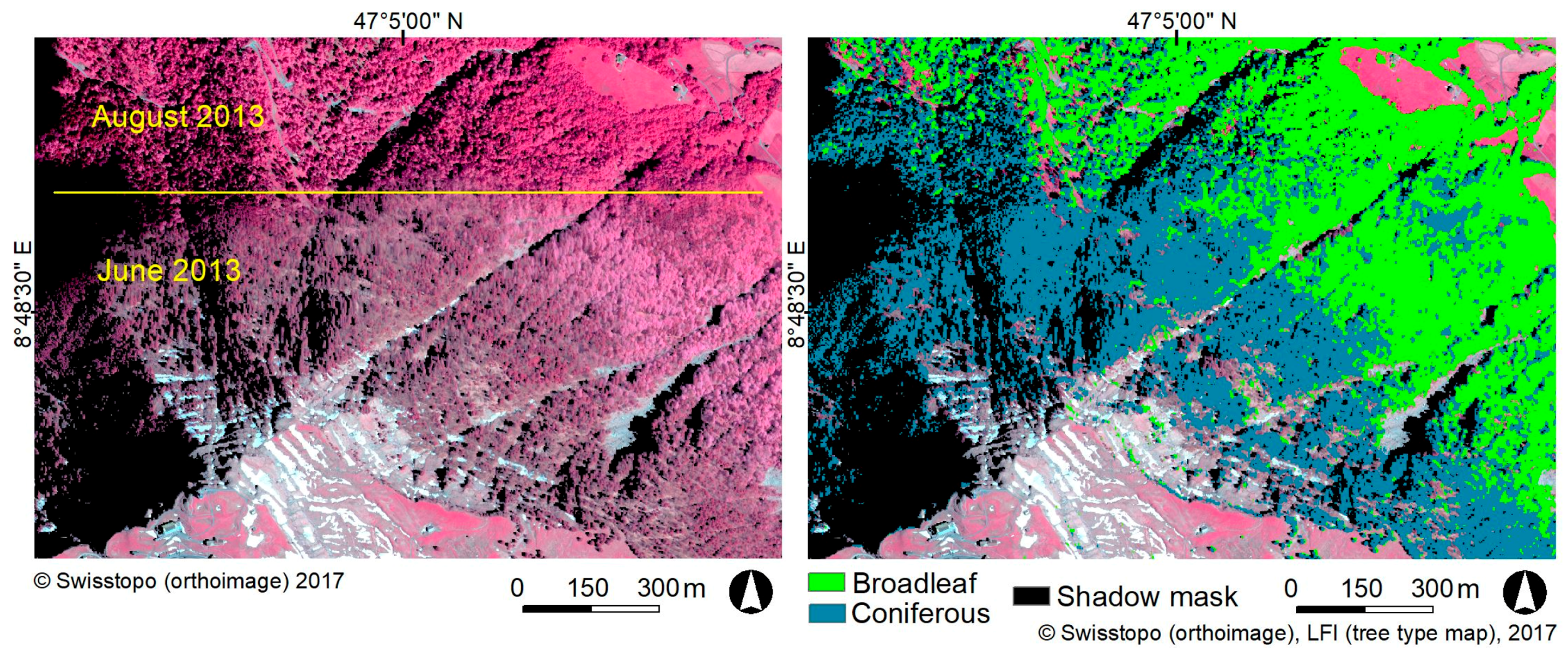
In contrast, using the two topographic variables elevation and aspect for the tree type classification partly reduced the spectral variability, in particular that of broadleaved trees. Large differences in elevation that occurred for image strips covering areas between approx. 400 m and 2000 m a.s.l. were satisfactorily compensated with the topographic variable elevation (see Figure 9). In contrast, by implementing the variable terrain exposition, errors of commission of coniferous tree types in north-oriented slopes were only marginally reduced. Figure 9 shows that additional rigorous masking of shadows was necessary. When focusing on large geographic extents, it would be more beneficial to reduce spectral variability by integrating topo-climatic variables into the classification approach [41].
Both the classification algorithm and unit (the 3-m regular raster) may also affect the tree type mapping approach. The stability of the RF classifier was an important criterion for its integration into operational settings and thus suitability for wall-to-wall applications [29]. Vetrivel et al. [58] reported that the overall classification accuracy of the RF classifier decreases when the algorithm is trained on different study areas. Juel et al. [59] tested the transferability of RF classification models for mapping vegetation from aerial images and DTMs and concluded that the resulting classification model was not transferable to new (similar) areas. However, this in contrast to our experience with the proposed tree type mapping approach. Regarding the classification unit applied, the assignment of tree crowns to a regular 3-m raster meant that in most cases, the raster cells, in particular at the forest edge, did not exactly fit the tree crowns. Thus, the exact crowns were not represented by the proposed method. Although image segmentation or individual tree crown delineation (ITC) algorithms have been well established at a case study level using multispectral data [7], they are less feasible for countrywide approaches, not only due to methodological limitations but also due to the fact that individual tree crowns are not the primary target of such data sets. Consequently, the tree type map is less accurate regarding the exact geographic position of tree types but is more suitable for the assessment of their fractions per area, e.g., per forest stand. Furthermore, Figure 10 shows that the tree type map is less suitable for linear tree patches, particularly single trees that grow outside the forest, i.e., along waterbodies and in agricultural and urban areas. This is related less to the proposed method itself and the sampling of training data and more to restrictions of the VHM [30], which is used as the final mask for the tree types. Waser et al. [3] concluded that both shadows and the VHM affect the tree mapping approach at the forest edge.
Finally, another constraint of the tree type map is its use for applications such as international forest reporting, that go beyond the distinction of broadleaved and coniferous trees [60]. Further distinction of tree species was not feasible due to the previously listed constraints and the missing training and reference data sets.
4.5. Operational Use of the Tree Type Map
The main benefits of the tree type map are manifold because it guarantees repeatable and objective results. The recently increasing countrywide acquisition of stereo-images by many European countries and the increasing availability of Sentinel imagery will make its future operational use more feasible. Restrictions are related less to acquisition of wall-to-wall imagery and the suggested classification approach and more to illumination and phenological constraints of the imagery and the spatial resolution of 3 m, which is too coarse for the exact shape of a tree crown. Nevertheless, the tree type map is suitable for the assessment of tree fractions per area (e.g., per forest stand or NFI plot, preferable within the forest) but not at the individual tree level. For the Swiss NFI, the obtained countrywide wall-to-wall tree type information makes it possible to densify the existing 1.4 km NFI sample plot grid for smaller areas of interest. It may also be used to optimize forest management and planning and could be important for the reliable assessment of forest resources studies. Furthermore, a countrywide, highly detailed tree type map may serve as an important information source for many other regional or national uses, such as avalanche or other hazard protection issues, as well as provide new perspectives for biodiversity or ecological connectivity studies (both flora and fauna).
4.6. Outlook
Further improvements to the tree type mapping approach are required to improve its suitability as a countrywide data set. Four points are essential.
First, to overcome problems that were directly related to the input imagery, an image-specific shadow masking could be applied. Likewise, a more harmonized timing of the acquisition between image strips, as well as limiting acquisition time to from the end of June to the end of August and around noon will improve the classification results. However, these limitations are not feasible as long as routinely acquired digital aerial imagery is used. Thus, the use of multi-temporal Sentinel data probably has the highest potential for further improving classification results, especially when dense time series are available [15]. Multi-temporal imagery of both ADS or Sentinel-2 imagery would also make further distinction of coniferous and broadleaved tree species more feasible—assuming that the required reference data are available. Moreover, the additional use of ALS or combining the tree type map approach with ALS data (leaf-off), provided that ALS maintains its popularity, would be beneficial for a better distinction between broadleaves and conifers in complex geographical locations.
Second, more effort is needed to further decrease the intra-class spectral variability. Depending on the overall number of samples available in a data set, one straightforward way to increase the representativeness of the data set while avoiding increased intra-class variability could be the definition of several reference classes per tree type (e.g., conifers on shaded and sunlit slopes, young and old stands). The use of such internal sub-classes has been found to be useful [61]. The classes can then be merged again in a post-classification step. This should also include minimizing shadows or classification of shaded areas (both cast and crown-internal shadows) as suggested by [7,12,61,62].
Third, future work is needed to further reduce the large amount of input data. The parameter “features’ importance” as provided by RF should be used as suggested by [44].
Fourth, future research is needed to improve the accuracy of the tree type map outside forests. This includes collection of additional training samples, more accurate representation of the tree crowns by adapting the classification unit, as well as a new concept for validation of these areas because NFI data are only available within the forest.
5. Conclusions
This study presents a wall-to-wall mapping approach of broadleaved and coniferous trees across Switzerland (41,285 km2) based on routinely acquired (six-year cycle) digital aerial imagery. The tree type map with a spatial resolution of 3 m provides detailed, accurate and up-to-date information on the forest composition of the entire country. The accuracy assessment revealed high model overall accuracies in the range of 0.95 to 0.99 and tolerable deviations between the predicted tree types and independent NFI data. The proposed method enables the production of high quality tree type maps for large areas and therefore adds to existing knowledge because only few countrywide approaches for mapping forest attributes exist. Comparisons with another existing data set of temperate forests in Europe revealed that the tree type map is superior to other wall-to-wall products for temperate forests with complex topography regarding spatial resolution, level of detail and accuracy. An optimized methodological workflow was achieved by pretesting different classifiers regarding model accuracies and computation time and by dividing the entire area into subsets. For Switzerland, which has a highly heterogeneous landscape ranging from the Central Plateau to the Alps, a large representative training sample and the implementation of topographic variables to cope with spectral variability of the tree types were required. For a quality assessment of the final map, the deviations between independent NFI data and the tree type map were statistically analyzed. Despite sub-optimal acquisition times of the imagery and the related topographic (negative) effects on the prediction, the proposed approach confirmed the high potential of airborne digital sensor data for countrywide mapping of broadleaved and coniferous trees. The tree type map might be useful for optimizing forest management and planning activities and is an important information source for applications outside the forestry sector.
Acknowledgments
This study was carried out in the framework of the Swiss National Forest Inventory (NFI), a cooperative effort between the Swiss Federal Institute for Forest, Snow and Landscape Research (WSL) and the Swiss Federal Office for the Environment (FOEN). We thank Adrian Lanz and Marco Mina for fruitful discussions on the statistical analysis and Melissa Dawes for professional language editing. Finally, we thank the two anonymous reviewers for helping us to improve the manuscript.
Author Contributions
Lars T. Waser is responsible for the study. He developed the tree type mapping methodology, pretesting and was the main writer of the manuscript. Nataliia Rehush performed the R programming, statistical analysis, and validation of results. Christian Ginzler was responsible for the pre-processing of the image data and the generation of the countrywide orthoimage.
Conflicts of Interest
The authors declare no conflict of interest.
Appendix A. Comparison with High Resolution Layer (HRL Forest 2012)

Table A1.
Measurements of agreement in predicted and observed broadleaved fractions in the IAs and the High Resolution Layers (HRL forest 2012) 20-m forest type map using Median (M), absolute Median (Mabs), Normalized Median Absolute Deviation (NMAD), and Root Mean Squared Error (RMSE). The validation incorporates all IAs, NFI production regions, NFI elevation levels, NFI stand composition (percentage of conifers), terrain exposition (aspect), location, and the presence of other land cover classes.
| Validation Based on | IAs (n) | M (%) | Mabs (%) | NMAD (%) | RMSE (%) |
|---|---|---|---|---|---|
| All IAs | 3210 | 0 | 12 | 17.79 | 34.83 |
| Production region | |||||
| Jura | 560 | 1.72 | 13.04 | 18.62 | 28.13 |
| Central Plateau | 657 | 0 | 17.2 | 25.5 | 32.34 |
| Prealps | 621 | −4.35 | 17.43 | 26.09 | 36.54 |
| Alps | 951 | 0 | 3.4 | 5.04 | 35.81 |
| Southern Alps | 419 | 0 | 8.4 | 12.45 | 41.27 |
| Elevation (m a.s.l.) | |||||
| <600 | 571 | 0 | 11.4 | 16.9 | 30.42 |
| 600–1000 | 1062 | 0 | 17.65 | 26.17 | 36.59 |
| 1001–1400 | 855 | −4.27 | 20 | 30.73 | 39.57 |
| 1401–1800 | 550 | 0 | 0 | 0 | 28.56 |
| >1800 | 172 | 0 | 0 | 0 | 30.09 |
| Terrain exposition * | |||||
| North | 917 | 0 | 12 | 17.79 | 35.19 |
| East | 778 | 0 | 13.33 | 19.76 | 34.13 |
| South | 716 | 0 | 12.5 | 18.53 | 33.84 |
| West | 799 | 0 | 10.78 | 15.98 | 35.93 |
| Conifers (%) | |||||
| 91–100 | 940 | 0 | 0 | 0 | 24.69 |
| 51–90 | 610 | −16.67 | 27.27 | 24.7 | 33.15 |
| 11–50 | 882 | 7.8 | 31.18 | 37.98 | 42.42 |
| 0–10 | 778 | 0 | 4.17 | 6.18 | 36.95 |
| Location | |||||
| At forest edge | 552 | 0 | 12.5 | 18.53 | 37.02 |
| Within forest | 2658 | 0 | 12 | 17.79 | 34.35 |
| Other land cover | |||||
| Present | 2787 | 0 | 12.34 | 18.3 | 34.68 |
| Not present | 423 | 0 | 12 | 17.79 | 35.75 |
* north: from 315 to 45 degrees; east: from 45 to 135 degrees; south: from 135 to 225 degrees; west: from 225 to 315 degrees.
References
- Straub, C.; Stepper, C.; Seitz, R.; Waser, L.T. Potential of UltraCamX stereo images for estimating timber volume and basal area at the plot level in mixed European forests. Can. J. For. Res. 2013, 43, 731–741. [Google Scholar] [CrossRef]
- Vihervaara, P.; Auvinen, A.P.; Mononen, L.; Törmä, M.; Ahlroth, P.; Anttila, S.; Böttcher, K.; Forsius, M.; Heino, J.; Heliölä, J.; et al. How essential biodiversity variables and remote sensing can help national biodiversity monitoring. Glob. Ecol. Conserv. 2017, 10, 43–59. [Google Scholar] [CrossRef]
- Waser, L.T.; Fischer, C.; Wang, Z.; Ginzler, C. Wall-to-wall forest mapping based on digital surface models from image-based point clouds and a NFI forest definition. Forests 2015, 6, 4510–4528. [Google Scholar] [CrossRef]
- European Environmental Agency (EEA). European Forest Types: Categories and Types for Sustainable Forest Management Reporting and Policy; No. EEA Technical Report No 9/2006; EEA: Copenhagen, Denmark, 2007; Available online: http://www.env-edu.gr/Documents/European%20forest%20types.pdf (accessed on 10 July 2017).
- White, J.C.; Coops, N.C.; Wulder, M.A.; Vastaranta, M.; Hilker, T.; Tompalski, P. Remote sensing technologies for enhancing forest inventories: A review. Can. J. Remote Sens. 2016, 42, 619–641. [Google Scholar] [CrossRef]
- Barrett, F.; McRoberts, R.E.; Tomppo, E.; Cienciala, E.; Waser, L.T. A questionnaire-based review of the operational use of remotely sensed data by national forest inventories. Remote Sens. Environ. 2016, 174, 279–289. [Google Scholar] [CrossRef]
- Fassnacht, F.E.; Latifi, H.; Sterenczak, K.; Modzelewska, A.; Lefsky, M.; Waser, L.T.; Straub, C.; Ghosh, A. Review of studies on tree species classification from remotely sensed data. Remote Sens. Environ. 2016, 186, 64–87. [Google Scholar] [CrossRef]
- Holmgren, J.; Persson, A. Identifying species of individual trees using airborne laser scanner. Remote Sens. Environ. 2004, 90, 415–423. [Google Scholar] [CrossRef]
- Magnussen, S.; Boudewyn, P.; Wulder, M.A. Contextual classification of Landsat TM images to forest inventory cover types. Int. J. Remote Sens. 2004, 25, 2421–2440. [Google Scholar] [CrossRef]
- Stabach, J.A.; Dabek, L.; Jensen, J.; Wang, Y.Q. Discrimination of dominant forest types for Matschie’s tree kangaroo conservation in Papua New Guinea using high resolution remote sensing data. Int. J. Remote Sens. 2009, 30, 405–422. [Google Scholar] [CrossRef]
- Stoffels, J.; Mader, S.; Hill, J.; Werner, W.; Ontrup, G. Satellite-based stand-wise forest cover type mapping using a spatially adaptive classification approach. Eur. J. For. Res. 2012, 131, 1071–1089. [Google Scholar] [CrossRef]
- Waser, L.T.; Ginzler, C.; Kuechler, M.; Baltsavias, E.; Hurni, L. Semi-automatic classification of tree species in different forest ecosystems by spectral and geometric variables derived from Airborne Digital Sensor (ADS40) and RC30 data. Remote Sens. Environ. 2011, 115, 76–85. [Google Scholar] [CrossRef]
- Heinzel, J.; Koch, B. Investigating multiple data sources for tree species classification in temperate forest and use for single tree delineation. Int. J. Appl. Earth Obs. Geoinform. 2012, 18, 101–110. [Google Scholar] [CrossRef]
- Dalponte, M.; Ørka, H.O.; Ene, L.T.; Gobakken, T.; Næsset, E. Tree crown delineation and tree species classification in boreal forests using hyperspectral and ALS data. Remote Sens. Environ. 2014, 140, 306–317. [Google Scholar] [CrossRef]
- Immitzer, M.; Vuolo, F.; Atzberger, C. First experience with Sentinel-2 data for crop and tree species classifications in Central Europe. Remote Sens. 2016, 8, 166. [Google Scholar] [CrossRef]
- Schumacher, J.; Nord-Larsen, T. Wall-to-wall tree type classification using airborne Lidar data and CIR images. Int. J. Remote Sens. 2014, 35, 3057–3073. [Google Scholar] [CrossRef]
- European Environmental Agency. CLC2006 Technical Guidelines; EEA Technical Report No 17/20072007; EEA: Copenhagen, Denmark, 2007; Available online: http://land.copernicus.eu/user-corner/technical-library/CLC2006_technical_guidelines.pdf (accessed on 10 July 2017).
- Bartholomé, E.; Belward, A.S. GLC2000: A new approach to global land cover mapping from Earth observation data. Int. J. Remote Sens. 2005, 26, 1959–1977. [Google Scholar] [CrossRef]
- Bontemps, S.; Van Bogaert, E.; Defourny, P.; Kalogirou, V.; Arino, O. GlobCover 2009—Products Description Manual, version 1.0.; EEA: Copenhagen, Denmark, 2010; Available online: http://due.esrin.esa.int/page_globcover.php (accessed on 10 July 2017).
- Channan, S.; Collins, K.; Emanuel, W.R. Global Mosaics of the Standard MODIS Land Cover Type Data; University of Maryland and the Pacific Northwest National Laboratory: College Park, MD, USA, 2014. Available online: http://glcf.umd.edu/data/lc/ (accessed on 10 July 2017).
- Congalton, R.G.; Jianyu, G.; Yadav, K.; Thenkabail, P.; Ozdogan, M. Global land cover mapping: A review and uncertainty analysis. Remote Sens. 2014, 6, 12070–12093. [Google Scholar] [CrossRef]
- European Environmental Agency (EEA). GIO Land High Resolution Layers (HRLs)—Summary of Product Specifications; EEA: Copenhagen, Denmark, 2012; Available online: http://land.copernicus.eu/pan-european/high-resolution-layers/forests/view (accessed on 10 July 2017).
- Kempeneers, P.; Sedano, F.; Seebach, L.; Strobl, P.; San-Miguel-Ayanz, J. Data fusion of different spatial resolution remote sensing images applied to forest-type mapping. IEEE Trans. Geosci. Remote Sens. 2011, 49, 4977–4986. [Google Scholar] [CrossRef]
- Brus, D.J.; Hengeveld, G.M.; Walvoort, D.J.J.; Goedhart, P.W.; Heidema, A.H.; Nabuurs, G.J.; Gunia, K. Statistical mapping of tree species over Europe. Eur. J. For. Res. 2012, 131, 145–157. [Google Scholar] [CrossRef]
- Abegg, M.; Brändli, U.-B.; Cioldi, F.; Fischer, C.; Herold-Bonardi, A.; Huber, M.; Keller, M.; Meile, R.; Rösler, E.; Speich, S.; et al. Fourth National Forest Inventory—Result Tables and Maps on the Internet for the NFI 2009–2013 (NFI4b); Swiss Federal Institute for Forest, Snow and Landscape Research WSL: Birmensdorf, Switzerland, 2014. [Google Scholar]
- Jensen, J.R. Introductory Digital Image Processing: A Remote Sensing Perspective; Prentice Hall: Upper Saddle River, NY, USA, 2005. [Google Scholar]
- Breiman, L. Random forests. Mach. Learn. 2001, 45, 5–32. [Google Scholar] [CrossRef]
- Hastie, T.; Tibshirani, R.; Friedman, J. The Elements of Statistical Learning: Data Mining, Inference, and Prediction, 2nd ed.; Springer: New York, NY, USA, 2009. [Google Scholar]
- Belgiu, M.; Drăguţ, L. Random forest in remote sensing: A review of applications and future directions. ISPRS J. Photogramm. Remote Sens. 2016, 114, 24–31. [Google Scholar] [CrossRef]
- Ginzler, C.; Hobi, M.L. Countrywide stereo-image matching for updating digital surface models in the framework of the Swiss National Forest Inventory. Remote Sens. 2015, 7, 4343–4370. [Google Scholar] [CrossRef]
- R Core Team. R: A Language and Environment for Statistical Computing; R Foundation for Statistical Computing: Vienna, Austria, 2017; Available online: https://www.R-project.org/ (accessed on 10 July 2017).
- Brändli, U.-B. Swiss National Forest Inventory: Results of the Third Assessment 2004–2006; Swiss Federal Institute for Forest, Snow and Landscape Research WSL: Birmensdorf, Switzerland, 2010; p. 312. [Google Scholar]
- Waser, L.T. Airborne Remote Sensing Data for Semi-Automated Extraction of Tree Area and Classification of Tree Species. Ph.D. Thesis, Dissertation 20464. Swiss Federal Institute of Technology ETH Zurich, Zürich, Switzerland, 2012. Available online: http://e-collection.library.ethz.ch/view/eth:6087 (accessed on 10 July 2017).
- Artuso, R.; Bovet, S.; Streilein, A. Practical methods for the verification of countrywide terrain and surface models. In Proceedings of the ISPRS Working Group III/3 Workshop XXXIV–3/W13. 3-D reconstruction from airborne laserscanner and InSAR data, Dresden, Germany, 8–10 October 2003. [Google Scholar]
- Mathys, L.; Ginzler, C.; Zimmermann, N.E.; Brassel, P.; Wildi, O. Sensitivity assessment on continuous landscape variables to classify a discrete forest area. For. Ecol. Manag. 2006, 229, 111–119. [Google Scholar] [CrossRef]
- Gonzales, R.C.; Woods, R.E. Digital Image Processing, 2nd ed.; Prentice Hall: New York, NY, USA, 2000. [Google Scholar]
- Schowengerdt, R.E. Remote Sensing: Models and Methods for Image Processing; Academic Press and Elsevier: Amsterdam, The Netherlands, 2006. [Google Scholar]
- Waser, L.T.; Küchler, M.; Jütte, K.; Stampfer, T. Evaluating the potential of WorldView-2 data to classify tree species and different levels of ash mortality. Remote Sens. 2014, 6, 4515–4545. [Google Scholar] [CrossRef]
- Bannari, A.; Morin, D.; Huette, A.R.; Bonn, F.A. A review of vegetation indices. Remote. Sens. Environ. 1995, 13, 95–120. [Google Scholar] [CrossRef]
- Qi, J.; Chehbouni, A.; Huete, A.R.; Kerr, Y.H.; Sorooshian, S. A modified soil adjusted vegetation index. Remote Sens. Environ. 1994, 48, 119–126. [Google Scholar] [CrossRef]
- Zimmermann, N.E.; Moisen, G.G.; Edwards, T.C.; Frescino, T.S.; Blackard, J.A. Remote sensing-based predictors improve distribution models of rare, early successional and broadleaved tree species in Utah. J. Appl. Ecol. 2007, 44, 1057–1067. [Google Scholar] [CrossRef] [PubMed]
- Engler, R.; Waser, L.T.; Zimmermann, N.E.; Schaub, M.; Berdos, S.; Ginzler, C.; Psomas, A. Combining ensemble modeling and remote sensing for mapping individual tree species at high spatial resolution. For. Ecol. Manag. 2013, 310, 64–73. [Google Scholar] [CrossRef]
- Criminisi, A.; Shotton, J.; Konukoglu, E. Decision Forests: A Unified Framework for Classification, Regression, Density Estimation, Manifold Learning and Semi-Supervised Learning; NOW Publishers: Breda, The Netherlands, 2012. [Google Scholar]
- Genuer, R.; Poggi, J.-M.; Tuleau-Malot, C. Variable selection using random forests. Pattern Recognit. Lett. 2010, 31, 2225–2236. [Google Scholar] [CrossRef]
- Pal, M. Random forest classifier for remote sensing classification. Int. J. Remote Sens. 2005, 26, 217–222. [Google Scholar] [CrossRef]
- Rodríguez-Galiano, V.F.; Chica-Olmo, M.; Abarca-Hernandez, F.; Atkinson, P.M.; Jeganathan, C. Random Forest classification of Mediterranean land cover using multi-seasonal imagery and multi-seasonal texture. Remote Sens. Environ. 2012, 121, 93–107. [Google Scholar] [CrossRef]
- Shao, J. Linear model selection by cross-validation. J. Am. Stat. Assoc. 1993, 88, 486–494. [Google Scholar] [CrossRef]
- Richter, K.; Atzberger, C.; Hank, T.B.; Mauser, W. Derivation of biophysical variables from earth observation data: Validation and statistical measures. J. Appl. Remote Sens. 2012, 6. [Google Scholar] [CrossRef]
- Kutner, M.H.; Nachtsheim, C.J.; Neter, J.; Li, W. Applied Linear Statistical Models, 5th ed.; McGraw-Hill: Irwin, NY, USA, 2004; 1369p. [Google Scholar]
- Höhle, J.; Höhle, M. Accuracy assessment of digital elevation models by means of robust statistical methods. ISPRS J. Photogramm. Remote Sens. 2009, 64, 398–406. [Google Scholar] [CrossRef]
- Dalponte, M.; Ørka, H.O.; Gobakken, T.; Gianelle, D.; Naesset, E. Tree species classification in boreal forests with hyperspectral data. IEEE Trans. Geosci. Remote Sens. 2013, 51, 2632–2645. [Google Scholar] [CrossRef]
- Colditz, R. An evaluation of different training sample allocation schemes for discrete and continuous land cover classification using decision tree-based algorithms. Remote Sens. 2015, 7, 9655. [Google Scholar] [CrossRef]
- Reese, H.; Nilsson, M.; Granqvist Pahlén, T.; Hagner, O.; Joyce, S.; Tingelöf, U.; Egberth, M.; Olsson, H. Countrywide estimates of forest variables using satellite data and field data from the National Forest Inventory. AMBIO J. Hum. Environ. 2003, 32, 542–548. [Google Scholar] [CrossRef]
- Düggelin, C.H.; Keller, M. Swiss National Forest Inventory: Manual for Terrestrial Survey; Swiss Federal Institute for Forest, Snow and Landscape Research WSL: Birmensdorf, Switzerland, 2017; p. 220. [Google Scholar]
- Federal Statistical Office. Forest Degree of Mixture of Switzerland; Swiss Federal Statistical Office: Neuchatel, Switzerland, 2001; Available online: http://files.be.ch/bve/agi/geoportal/geo/lpi/WALDMI_1992_01_LANG_DE.PDF (accessed on 10 July 2017).
- Markelin, L.; Honkavaara, E.; Schlaepfer, D.; Bovet, S.T.; Korpela, I. Assessment of radiometric correction methods for ADS40 imagery. Photogramm. Fernerkund. Geoinform. 2012, 3, 251–266. [Google Scholar] [CrossRef] [PubMed]
- Richter, R.; Schläpfer, D. Atmospheric/Topographic Correction for Airborne Imagery; DLR report DLR-IB 565-02/14; DLR: Wessling, Germany, 2014; p. 240.
- Vetrivel, A.; Gerke, M.; Kerle, N.; Vosselman, G. Identification of damage in buildings based on gaps in 3D point clouds from very high resolution oblique airborne images. ISPRS J. Photogramm. Remote Sens. 2015, 105, 61–78. [Google Scholar] [CrossRef]
- Juel, A.; Groom, G.B.; Svenning, J.-C.; Ejrnæs, R. Spatial application of random forest models for fine-scale coastal vegetation classification using object based analysis of aerial orthophoto and DEM data. Int. J. Appl. Earth Obs. Geoinform. 2015, 42, 106–114. [Google Scholar] [CrossRef]
- Barbati, A.; Marchetti, M.; Chirici, G.; Corona, P. European Forest Types and Forest Europe SFM indicators: Tools for monitoring progress on forest biodiversity conservation. For. Ecol. Manag. 2014, 321, 145–157. [Google Scholar] [CrossRef] [Green Version]
- Leckie, D.G.; Tinis, S.; Nelson, T.; Burnett, C.; Gougeon, F.A.; Cloney, E.; Paradine, D. Issues in species classification of trees in old growth conifer stands. Can. J. Remote Sens. 2005, 31, 175–190. [Google Scholar] [CrossRef]
- Leckie, D.G.; Gougeon, F.A.; Walsworth, N.; Paradine, D. Stand delineation and composition estimation using semi-automated individual tree crown analysis. Remote Sens. Environ. 2003, 85, 355–369. [Google Scholar] [CrossRef]
Figure 1.
Workflow of the countrywide tree type classification approach.
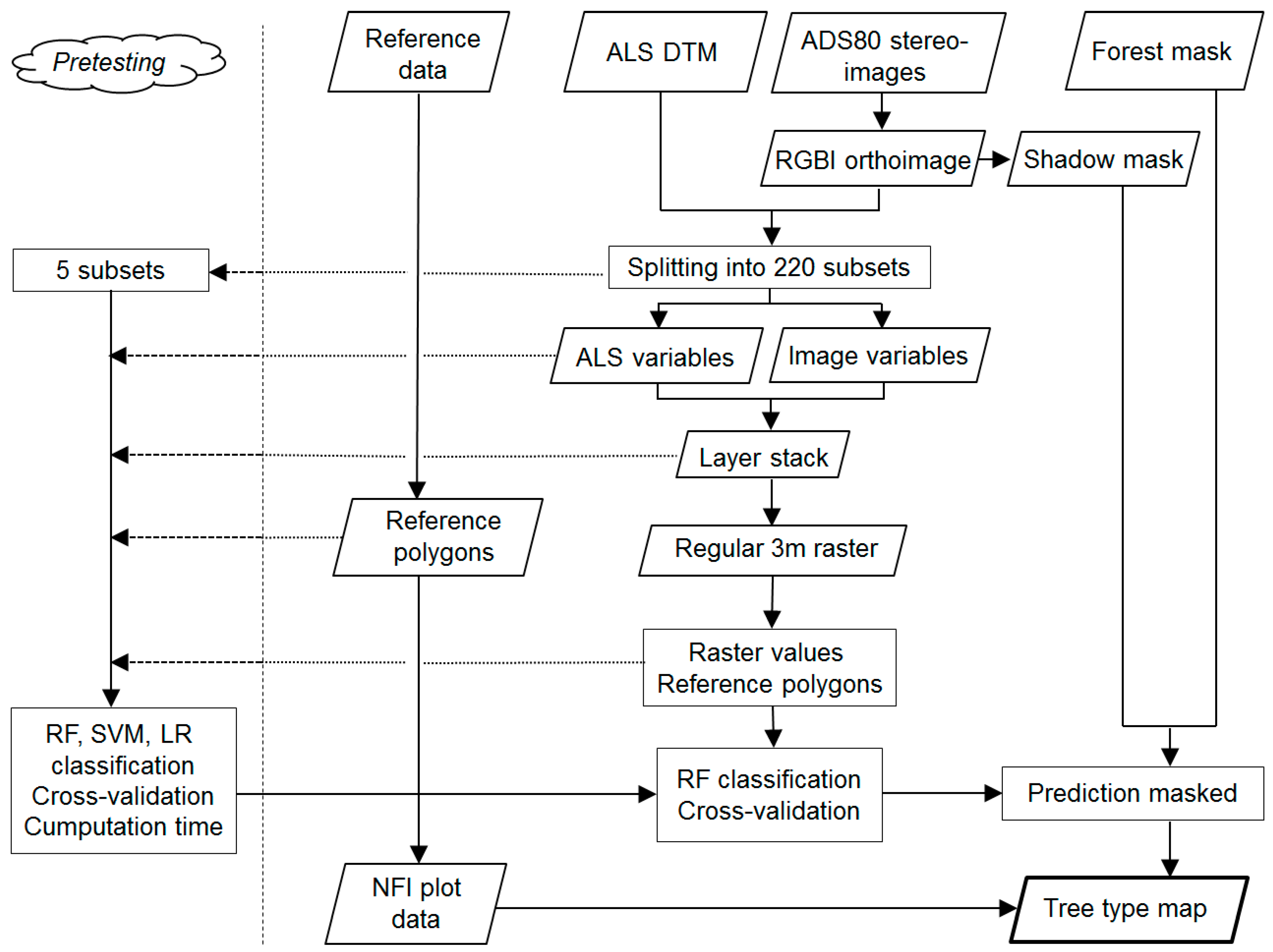
Figure 2.
Area of Switzerland with the 220 subsets and the 5 Swiss National Forest Inventory (NFI) forest production regions.
Figure 2.
Area of Switzerland with the 220 subsets and the 5 Swiss National Forest Inventory (NFI) forest production regions.
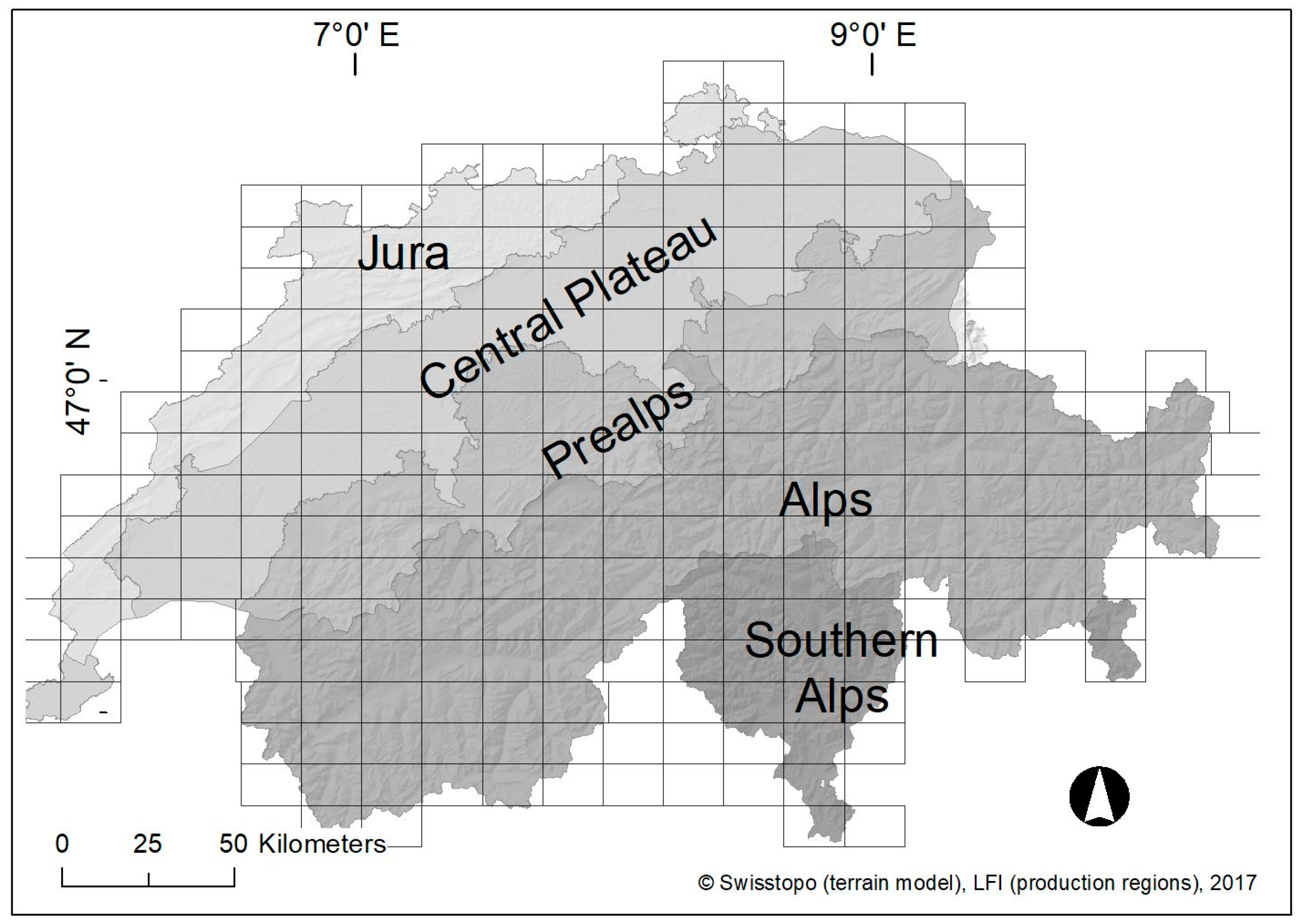
Figure 3.
Interpretation of the 25 sub-sampling points (Right) of a 1.4 km regular raster; (Left) for coniferous (green) and broadleaved (light green) tree type decisions.
Figure 3.
Interpretation of the 25 sub-sampling points (Right) of a 1.4 km regular raster; (Left) for coniferous (green) and broadleaved (light green) tree type decisions.
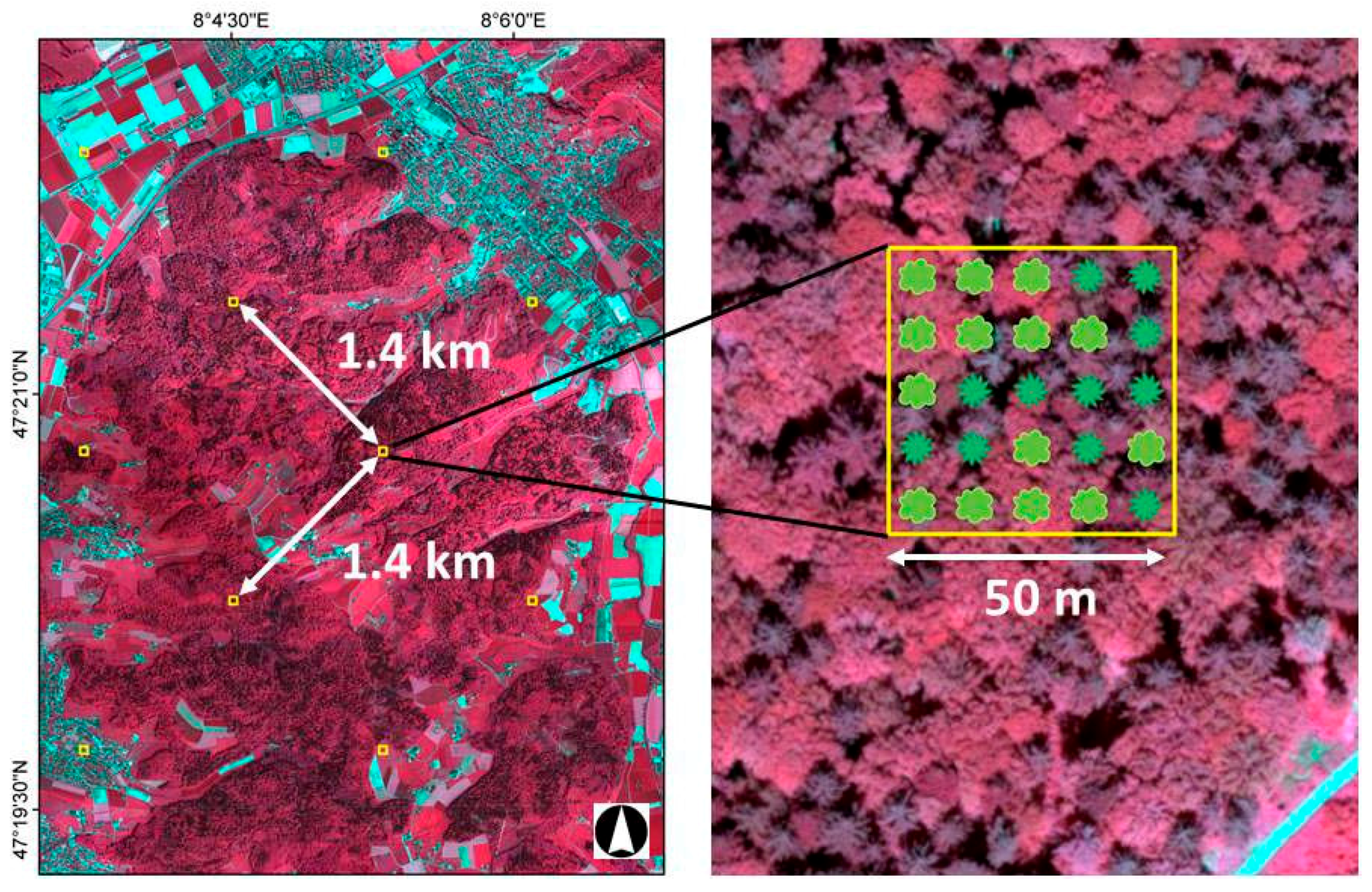
Figure 4.
Distribution of the overall accuracies and kappa values of 220 subsets, based on the model results for the five NFI production regions. Number of subsets is given in brackets. Results were obtained using 10-fold cross-validation repeated five times.
Figure 4.
Distribution of the overall accuracies and kappa values of 220 subsets, based on the model results for the five NFI production regions. Number of subsets is given in brackets. Results were obtained using 10-fold cross-validation repeated five times.
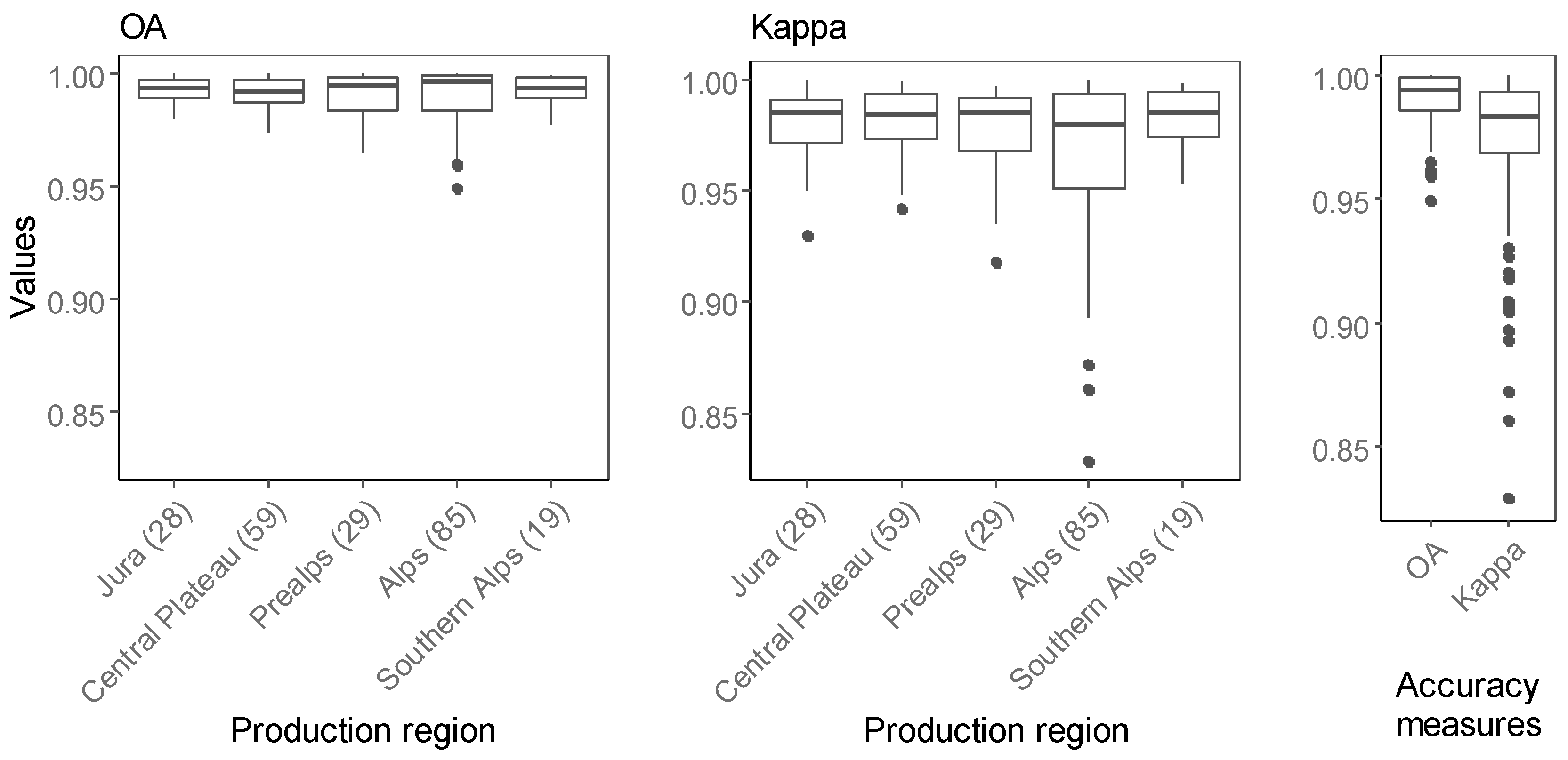
Figure 5.
Tree type map of Switzerland with the distinction between broadleaved and coniferous trees.
Figure 5.
Tree type map of Switzerland with the distinction between broadleaved and coniferous trees.
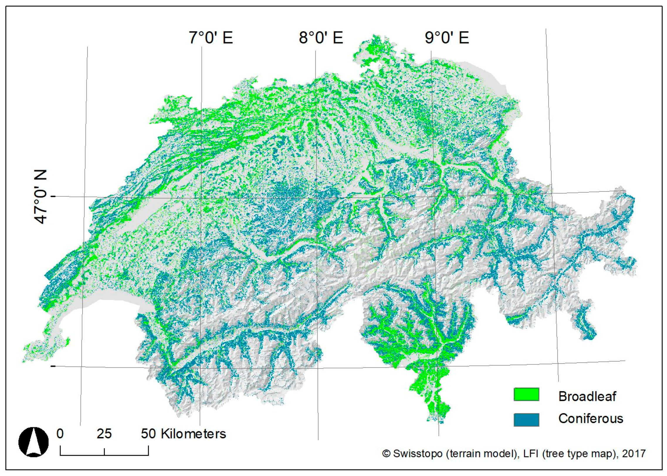
Figure 6.
Histogram of the deviation values in predicted (tree type map) and observed (NFI image interpretation) broadleaved fraction in the IAs.
Figure 6.
Histogram of the deviation values in predicted (tree type map) and observed (NFI image interpretation) broadleaved fraction in the IAs.

Figure 7.
Deviation in predicted (tree type map) and observed (NFI image interpretation) broadleaved fraction in the IAs.
Figure 7.
Deviation in predicted (tree type map) and observed (NFI image interpretation) broadleaved fraction in the IAs.
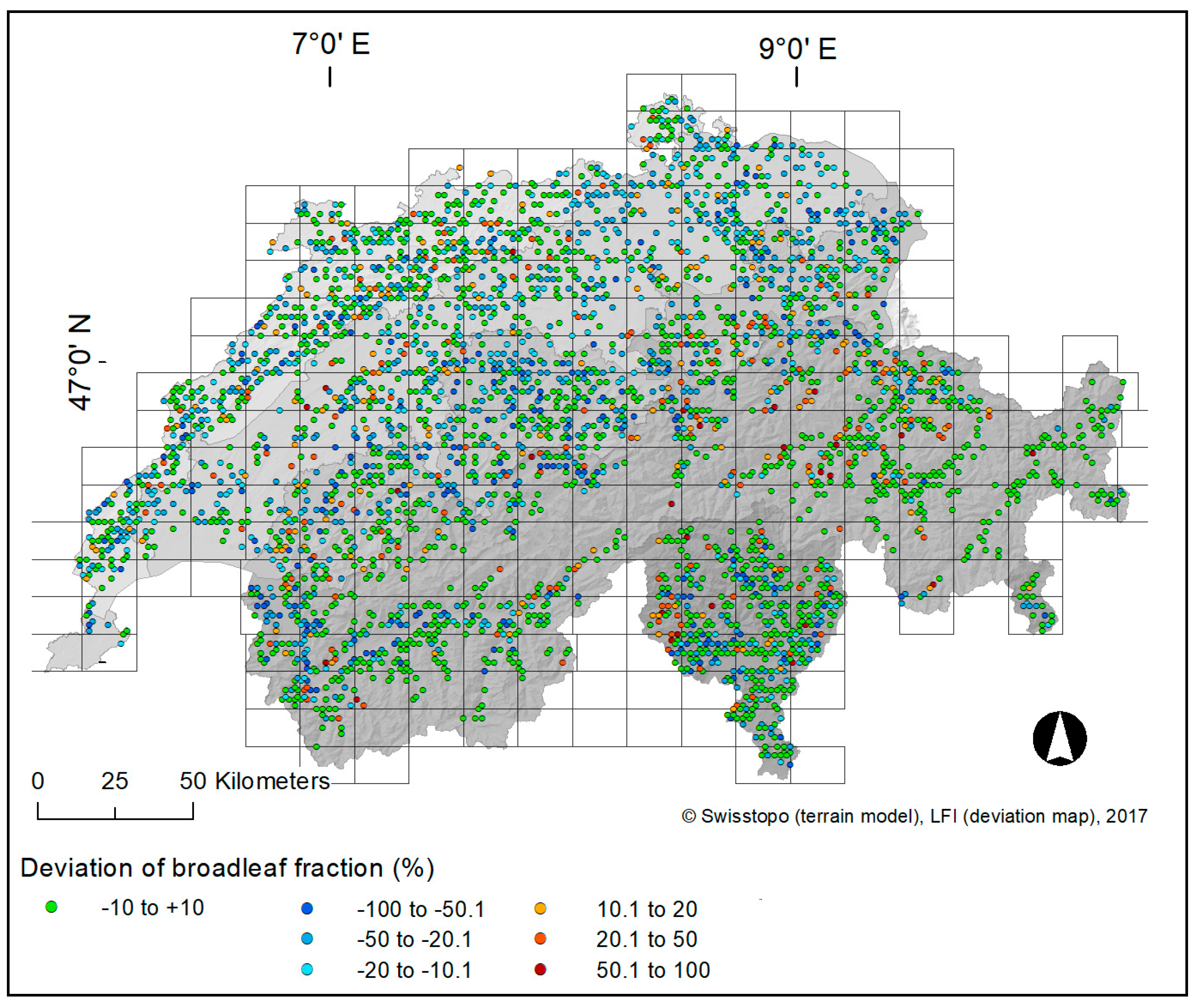
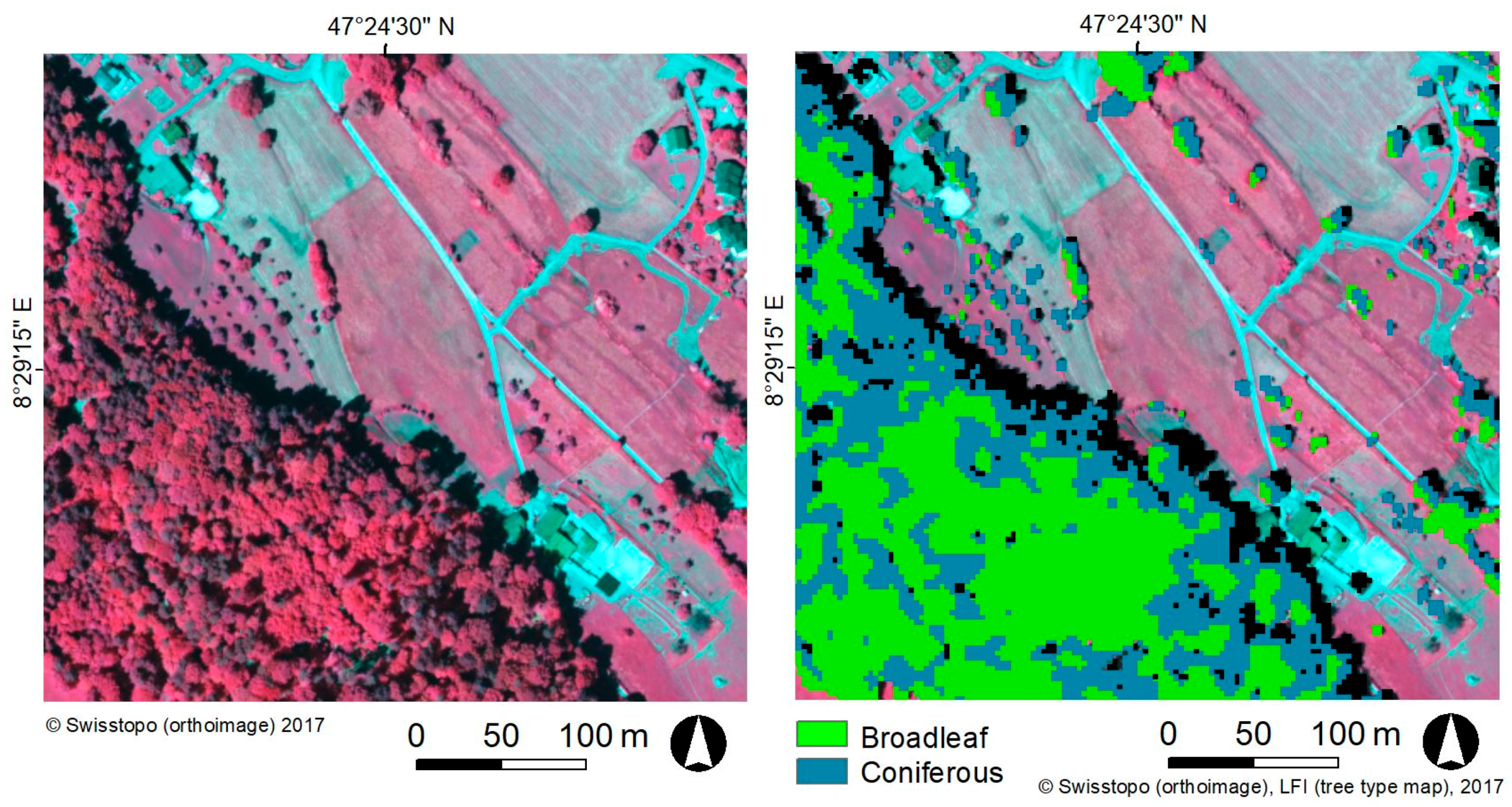
Figure 8.
(a–c) Differences in tree types and level of detail between the tree type map (b) and the High Resolution Layers (c). The CIR orthoimage (a) is given as a reference, where coniferous trees appear darker red than broadleaved trees.
Figure 8.
(a–c) Differences in tree types and level of detail between the tree type map (b) and the High Resolution Layers (c). The CIR orthoimage (a) is given as a reference, where coniferous trees appear darker red than broadleaved trees.

Figure 9.
Illustration of several constraints of the tree mapping approach. CIR aerial image of a part of a subset in the Prealps (Left) that consists of two different images from different dates, with clear differences in the appearance of the broadleaved and coniferous trees. Rigorous shadow masking (black) and the implementation of topographic variables enabled a reasonable prediction of the tree types (Right).

Figure 10.
Example of a CIR aerial image of mixed forests in the Central Plateau (Left); The tree type map (Right) shows an overestimation of conifers for small or linear tree patches (in the middle of the image) and partly at the forest edge of mixed forests in shaded and north-oriented slopes (right bottom corner of the image).

Table 1.
Technical specifications of the two ADS sensors, as used by Swisstopo for the countrywide image acquisition.
Table 1.
Technical specifications of the two ADS sensors, as used by Swisstopo for the countrywide image acquisition.
| Parameter | ADS40-SH52; ADS80-SH82 |
|---|---|
| Time of operation | 2008–present; 2009–present |
| Sensor | Three-line CCD scanner |
| Dynamic range of the CCD | 12-bit |
| Spectral bands (nm) | Panchromatic 465–680 |
| Blue 428–492 | |
| Green 533–587 | |
| Red 608–662 | |
| Near infrared 833–887 | |
| CCD elements | 12 CCD lines with 12,000 pixels each |
| Pixel size (μm) | 6.5 |
Table 2.
Tree types sampled. The number of polygons refers to the delineated reference polygons, whereas the number of assigned grid cells refers to the corresponding grid cells in the 3-m regular raster.
Table 2.
Tree types sampled. The number of polygons refers to the delineated reference polygons, whereas the number of assigned grid cells refers to the corresponding grid cells in the 3-m regular raster.
| Tree Type | Number of Delineated Polygons | Average Area (m2) | Min Area (m2) | Max Area (m2) | Number of Assigned Grid Cells (9 m2) |
|---|---|---|---|---|---|
| broadleaved | 112,940 | 701.8 | 36.1 | 10,290 | 1,144,200 |
| coniferous | 72,300 | 464.3 | 7.5 | 8081 | 770,340 |
| ∑ | 185,240 | 1,914,540 |
Table 3.
Summary of the pretesting using the five subsets. For the three classifiers Logistic Regression Model (LRM), Support Vector Machine (SVM), and Random Forest (RF), the obtained overall accuracies (OA), computing time in minutes, and the number of delineated polygons are given. The models were 10-fold cross-validated.
| Subset | LRM | SVM | RF | Number of Delineated Polygons | |||
|---|---|---|---|---|---|---|---|
| OA | Time (min) | OA | Time (min) | OA | Time (min) | ||
| 1 | 0.989 | 132 | 0.985 | 219 | 0.991 | 105 | 922 |
| 2 | 0.988 | 122 | 0.987 | 230 | 0.988 | 109 | 1026 |
| 3 | 0.987 | 112 | 0.982 | 211 | 0.989 | 110 | 998 |
| 4 | 0.989 | 105 | 0.988 | 201 | 0.986 | 87 | 840 |
| 5 | 0.993 | 123 | 0.986 | 168 | 0.992 | 99 | 905 |
Table 4.
Summary of the paired t-test for LRM, SVM and RF for both OA and computing time. Statistical significance is given as follows: *** p < 0.001; ** p < 0.01; * p < 0.05.
Table 4.
Summary of the paired t-test for LRM, SVM and RF for both OA and computing time. Statistical significance is given as follows: *** p < 0.001; ** p < 0.01; * p < 0.05.
| Classifier | OA | Time | ||
|---|---|---|---|---|
| SVM | RF | SVM | RF | |
| LRM | 0.03568 * | 0.6313 | 0.001419 ** | 0.02618 * |
| RF | 0.1457 | - | 0.000369 *** | - |
Table 5.
Measurements of agreement in predicted and observed broadleaved fractions in the IAs using Median (M), absolute Median (Mabs), Normalized Median Absolute Deviation (NMAD), and Root Mean Squared Error (RMSE). The validation incorporates all IAs, NFI production regions, NFI elevation levels, NFI stand composition (percentage of conifers), terrain exposition (aspect), location, and the presence of other land cover classes, and time lag.
| Validation Based on | IAs (n) | M (%) | Mabs (%) | NMAD (%) | RMSE (%) |
|---|---|---|---|---|---|
| All IAs | 3373 | −3.17 | 9.75 | 13.82 | 26.51 |
| Production region | |||||
| Jura | 577 | −6.08 | 10.53 | 15.86 | 22.31 |
| Central Plateau | 693 | −11.17 | 14.08 | 17.14 | 25.6 |
| Prealps | 653 | −6.27 | 13.08 | 17.89 | 29.47 |
| Alps | 1016 | 0 | 4.57 | 6.78 | 26.29 |
| Southern Alps | 432 | 0 | 6.33 | 9.38 | 28.83 |
| Elevation (m a.s.l.) | |||||
| <600 | 608 | −9.98 | 13.25 | 15.98 | 27.25 |
| 600–1000 | 1109 | −10.55 | 15.54 | 20.03 | 29.57 |
| 1001–1400 | 899 | −3.98 | 11.91 | 18.01 | 28.77 |
| 1401–1800 | 575 | 0 | 0.93 | 1.38 | 17.75 |
| >1800 | 182 | 0 | 0 | 0 | 11.4 |
| Terrain exposition * | |||||
| North | 945 | −8.33 | 13.18 | 17.3 | 30.41 |
| East | 825 | −1.49 | 9.45 | 13.55 | 24.04 |
| South | 780 | 0 | 8.45 | 12.53 | 21.25 |
| West | 823 | −3.62 | 9.08 | 12.11 | 28.47 |
| Conifers (%) | |||||
| 91–100 | 973 | 0 | 0 | 0 | 11.99 |
| 51–90 | 620 | −10.4 | 14.86 | 17.33 | 21.84 |
| 11–50 | 914 | −15.46 | 19.84 | 28.55 | 31.89 |
| 0–10 | 866 | −11.46 | 11.46 | 16.98 | 34.06 |
| Location | |||||
| At forest edge | 654 | −6.73 | 13.53 | 18.11 | 29.43 |
| Within forest | 2719 | −2.2 | 8.9 | 13.08 | 25.75 |
| Other land cover | |||||
| Present | 2930 | −2.7 | 9.64 | 13.65 | 26.42 |
| Not present | 443 | −5.22 | 10.56 | 15.51 | 27.06 |
| Time lag (years) | |||||
| ≤1 | 214 | −7.29 | 12.25 | 16.11 | 21.47 |
| 2–5 | 1382 | −2.29 | 9.02 | 13.19 | 25.92 |
| 6–10 | 1777 | −3.23 | 10.06 | 13.91 | 27.5 |
* north: from 315 to 45 degrees; east: from 45 to 135 degrees; south: from 135 to 225 degrees; west: from 225 to 315 degrees.
Table 6.
Output of a model testing the influence of different parameters on the tree type map validation using multiple linear regression. The multiple linear regression was based on the IAs with at least nine points interpreted as trees and resulted in an adjusted R-squared of 0.18. For the categorical predictors, the following reference categories were chosen: production region—Jura, terrain exposition—north, location—in forest, other classes of land cover—present, and time lag ≤ 1 year. Statistical significance is given as follows: *** p < 0.001; ** p < 0.01; * p < 0.05.
| Predictors | Estimate | Std. Error | t-Value | p-Value |
|---|---|---|---|---|
| Production region | ||||
| Central Plateau | 2.6903 | 1.0844 | 2.4808 | <0.05 * |
| Prealps | 9.3935 | 1.1034 | 8.5129 | <0.001 *** |
| Alps | 7.412 | 1.0986 | 6.7468 | <0.001 *** |
| Southern Alps | 3.4867 | 1.2384 | 2.8155 | <0.01 ** |
| Terrain exposition | ||||
| East | −5.4801 | 0.8791 | −6.2338 | <0.001 *** |
| South | −7.5935 | 0.8934 | −8.4996 | <0.001 *** |
| West | −2.9419 | 0.8777 | −3.3517 | <0.001 *** |
| Elevation (m a.s.l.) | −1.1156 | 0.5413 | −2.061 | <0.05 * |
| Conifers (%) | 7.2667 | 0.3932 | 18.48 | <0.001 *** |
| Location | ||||
| At forest edge | −0.214 | 0.961 | −0.2227 | >0.05 |
| Other land cover classes | ||||
| Present | 3.8572 | 1.0464 | 3.6861 | <0.001 *** |
| Time lag (years) | ||||
| 2–5 | 1.6598 | 1.3711 | 1.2106 | >0.05 |
| 6–10 | 3.1206 | 1.3573 | 2.2991 | <0.05 * |
© 2017 by the authors. Licensee MDPI, Basel, Switzerland. This article is an open access article distributed under the terms and conditions of the Creative Commons Attribution (CC BY) license (http://creativecommons.org/licenses/by/4.0/).
Share and Cite
MDPI and ACS Style
Waser, L.T.; Ginzler, C.; Rehush, N. Wall-to-Wall Tree Type Mapping from Countrywide Airborne Remote Sensing Surveys. Remote Sens. 2017, 9, 766. https://doi.org/10.3390/rs9080766
AMA Style
Waser LT, Ginzler C, Rehush N. Wall-to-Wall Tree Type Mapping from Countrywide Airborne Remote Sensing Surveys. Remote Sensing. 2017; 9(8):766. https://doi.org/10.3390/rs9080766
Chicago/Turabian StyleWaser, Lars T., Christian Ginzler, and Nataliia Rehush. 2017. "Wall-to-Wall Tree Type Mapping from Countrywide Airborne Remote Sensing Surveys" Remote Sensing 9, no. 8: 766. https://doi.org/10.3390/rs9080766
Note that from the first issue of 2016, this journal uses article numbers instead of page numbers. See further details here.