On the Objectivity of the Objective Function—Problems with Unsupervised Segmentation Evaluation Based on Global Score and a Possible Remedy

Abstract

Image segmentation is a crucial stage at the very beginning of many geographic object-based image analysis (GEOBIA) workflows. While segmentation quality is generally deemed of great importance, selecting adequate tuning parameters for a segmentation algorithm can be tedious and subjective. Procedures to automatically choose parameters of a segmentation algorithm are meant to make the process objective and reproducible. One of those approaches, and perhaps the most frequently used unsupervised parameter optimization method in the context of GEOBIA is called the objective function, also known as Global Score. Unfortunately, the method exhibits a hitherto widely neglected, yet severe source of instability, which makes quality rankings inconsistent. We demonstrate the issue in detail and propose a modification of the Global Score to mitigate the problem. This hopefully serves as a starting point to spark further development of the popular approach.

1. Introduction

Image segmentation is one of the first stages in geographic object based image analysis (GEOBIA). It is performed with the objective to partition an image into meaningful groups of pixels, i.e., the geo-objects depicted in an image. The quality of the segments is deemed crucial, as it will affect the performance of subsequent processing, especially the possibility to assign meaningful class labels to objects [1].

Image segmentation is regarded a hard problem in computer vision, due to its ill-posed nature [2,3]. By changing a segmentation algorithm’s tuning parameters or by altering the pre-processing of the input imagery, it is possible to produce a vast number of different segmentations for an image. Manually checking a large number of candidate solutions is possible and potentially leads to satisfying results [4], but is inherently time consuming and subjective in nature.

To ease the choice of a specific segmentation for further analysis, segmentation evaluation measures have been developed that can be used to optimize a segmentation algorithm’s input parameter values in an automated way [5,6,7,8,9,10,11,12]. One of the most popular unsupervised segmentation evaluation methods in remote sensing is called the Global Score (GS) [13] or simply objective function. The GS method was proposed by Espindola et al. [5]. GS combines measures of intra-segment homogeneity and inter-segment heterogeneity to judge segmentation quality. The former is expressed by the segments’ average variance weighted by its area, while the latter is expressed as the segments’ spatial autocorrelation in terms of Moran’s I [14,15]. In the original formulation of GS, the individual measures are calculated for a set of segmentations and a single image band. Intra-segment homogeneity and inter-segment heterogeneity measures are afterwards normalized separately to a common range (e.g., 0 to 1). The sum of the two normalized measures finally yields the objective function’s value.

The approach described above and variations thereof have been used in numerous studies in recent years [16,17,18,19,20,21,22,23,24,25,26,27,28]. Considerable efforts have been made to extend the original approach, e.g., to use multiple bands of input imagery [13,16], to consider optima at multiple scales [20,29,30], or to use GS for class specific optimization [26].

Unfortunately, however, the method has an inherent instability introduced by the normalization procedure. To the best of our knowledge, this inherent instability has not yet been treated in detail. While the purpose of parameter optimization is to make the choice of segmentation reproducible and less subjective, the calculation of GS in its current form exhibits an undesirable sensitivity to the user-defined range of parameters. The range of initial segmentation parameters is usually chosen ad-hoc and not sufficiently reasoned.

The aim of this work is to demonstrate the issue in detail. This helps to better understand the underlying causes of the problem, and to increase the general awareness. Based on this analysis, we provide a possible modification of the GS, mitigating the undesirable instability of the objective function.

2. Materials and Methods

To illustrate the effect of the different approaches, a set of candidate segmentations is obtained using the well-known Multiresolution Segmentation (MRS) algorithm [31]. MRS is a bottom-up region merging algorithm. Although we use MRS to illustrate our research, it has to be noted that the choice of segmentation algorithm itself does not affect the findings of our study.

The segmentations used here are produced leaving two of the three main parameters of MRS, namely Shape and Compactness, at constant levels of 0.1 and 0.5, respectively. The third parameter, called Scale, is altered in a range from 20 to 300 with an increment of 10, yielding a total of twenty-nine segmentations to illustrate the findings. The minimum and maximum Scale values ensure both, over- and under-segmentation.

Tests were performed on a Landsat dataset of the study area Assis microregion (São Paulo State, Brazil), available from a previous study [32]. The data cover roughly 715,000 ha of an agriculturally dominated landscape. Segmentation was initially performed on the full layer stack of six bands. For the sake of simplicity, and without the loss of generality, we restrict analysis here to a single band of the dataset (i.e., near-infrared band of Landsat 8 OLI). Similar findings will be obtained for each layer in the stack (not shown).

Global Score (GS) is a combination of area-weighted variance ($v$), measuring intra-segment homogeneity, and a measure of spatial autocorrelation, i.e., Moran’s I ($I$), globally quantifying similarity of neighboring segments. For a single band of an image, $v$ is calculated as:

$$v=\frac{{{\displaystyle \sum }}_{i=1}^n{a}_i*v_i}{{{\displaystyle \sum }}_{i=1}^n{a}_i},$$

(1)

where $n$ is the total number of segments and $v_i$ and $a_i$ are the variance and area of i segments, respectively. Calculation of Moran’s $I$ for a single band of an image is given by (see Figure 1 for illustration):

$$I=\frac{n {{\displaystyle \sum }}_{i=1}^n{{\displaystyle \sum }}_{j=1}^n{w}_{ij}\left(y_i-\overline{y}\right)\left(y_j-\overline{y}\right)}{({{\displaystyle \sum }}_{i=1}^n{(y_i-\overline{y})}^2)({{\displaystyle \sum }}_{i\ne j}{{\displaystyle \sum }}^{\text{}}{w}_{ij}))},$$

(2)

with $y_i$ and $y_j$ being the mean digital number of regions $R_i$ and $R_j$, respectively, and $\overline{y}$ the mean of variable $y$. Furthermore, $w_{ij}$ is a measure of the spatial contiguity of two regions $R_i$ and $R_j$. Following Espindola et al. [5], $w_{ij}$ is set to 1 for regions that share a common boundary and 0 for non-adjacent regions.

The individual measures of $I$ and $v$ are normalized to a common range from 0 to 1 in order to balance their relative importance. Normalization of $v$ and $I$ is performed either by the formula used in Espindola et al. [5]:

$$\frac{X_{max}-X}{X_{max}-X_{min}} ,$$

(3)

or the one used in Johnson and Xie [13]:

$$\frac{X- X_{min}}{X_{max}-X_{min}} .$$

(4)

Both are functionally equivalent; only the direction of optimization is different, i.e., minimization or maximization. We will use the latter, because it makes the shape of $I$ and $v$ more intuitive. Analogue findings would be obtained using Espindola’s normalization. The value of the objective function is finally the sum of the two normalized measures:

$$GS=v_{norm}+I_{norm}.$$

(5)

For multiband images, it has furthermore been proposed to average the GS calculated for each band individually [13,16].

3. Results

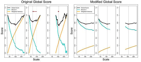
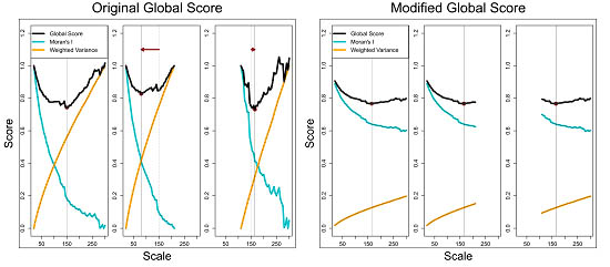
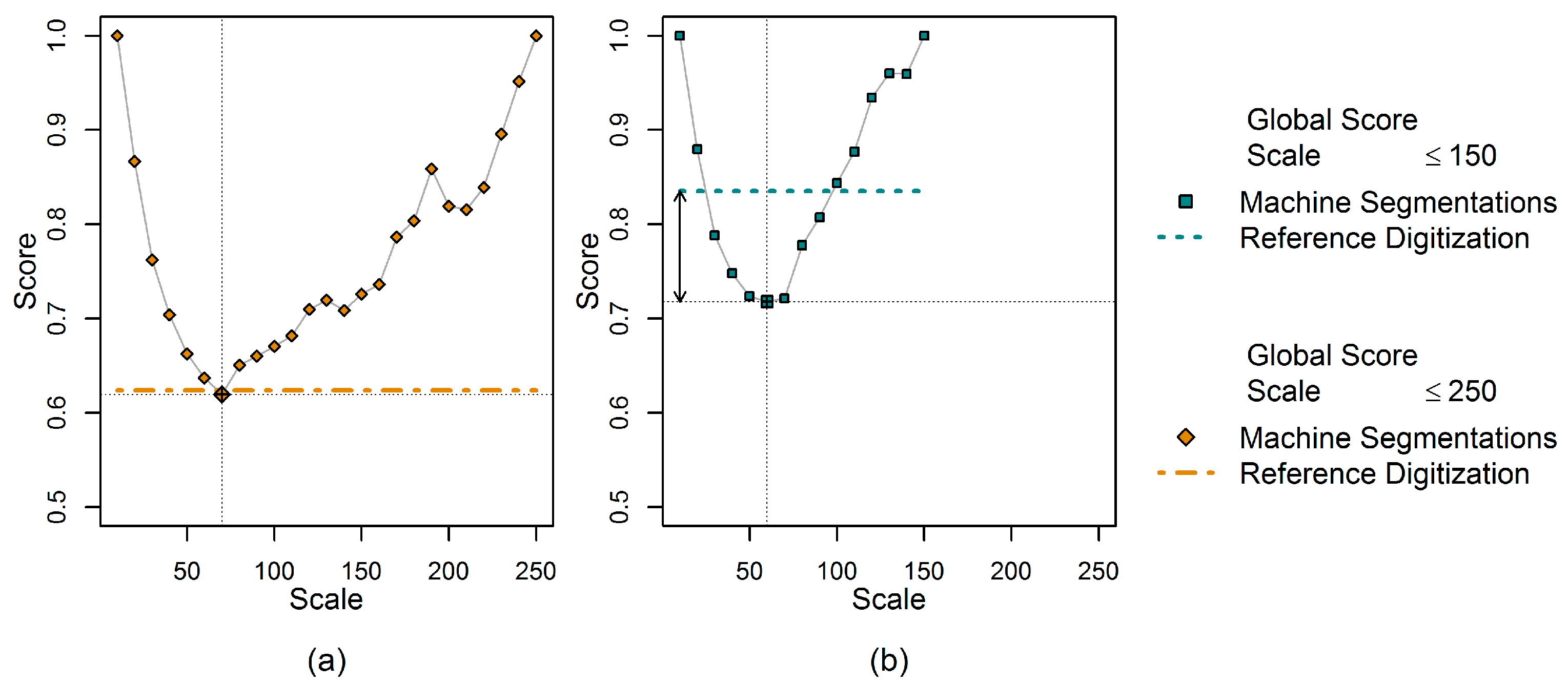
3.1. Illustration of the Sensitivity of GS to the User-Defined Range of Tested Segmentations

Area weighted variance typically increases as segments grow larger. By contrast, correlation between adjacent regions initially declines with growing size (yielding weaker spatial autocorrelation in terms of Moran’s I), but is expected to increase when segments become large enough to contain a mixture of classes [33]. As$v$ and I increase/decrease with increasing Scale parameter, the minimum and maximum values of the measures ($X_{min}$ and $X_{max}$) are likely to be attained by the finest and the coarsest segmentations in the test set, respectively. This is important, as minima and maxima are used afterwards to normalize the two components of Equation (5). The optimum of GS therefore depends on the user-defined range of parameters tested.

The net effect of variable $X_{min}$ and $X_{max}$ can easily be demonstrated, by calculating GS for the full set of candidate segmentations (Figure 2b) and two subsets separately (Figure 2a,c).

In the example provided in Figure 2, altering the range of segmentations used for analysis not only alters the absolute value of GS but also shifts the optimum. This would also occur, if all three parameters were varied and/or if another segmentation algorithm would have been chosen (not shown). Furthermore, comparison of GS in Figure 2a,c for Scale values between 110 and 210 shows inconsistencies in the relative ranking of segmentations’ ‘quality’. For example, segmentation at Scale 130 is more favorable than segmentation at Scale 190 according to Figure 2a, while the opposite is true in Figure 2c. The deplorable effects of using variable (range dependent) $X_{min}$ and $X_{max}$ are thus threefold:

• the absolute values of GS change,
• the optimum (minimum) value of GS is shifted,
• the relative ranking of acceptable candidate solutions is altered.

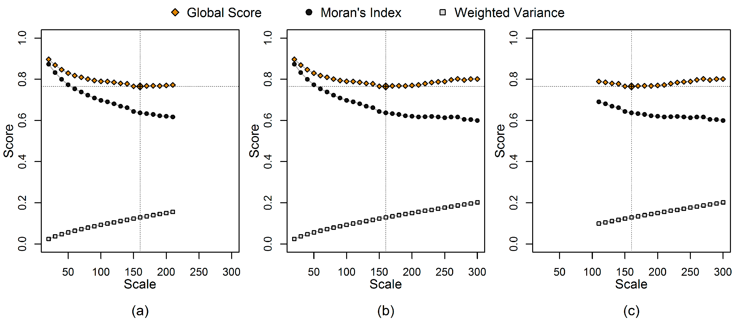
3.2. Illustration of an Alternative Normalization Scheme

Instead of using the minima and maxima ($X_{min}$, $X_{max}$) derived from the user-defined segmentations, we propose to normalize $I$ and $v$ to a fixed range prior to combination for GS. For $v$, the outmost limit of any segmentation for an image can be used. That is on one hand the situation, where each pixel resembles a segment on its own (complete over-segmentation) and the state where the entire image is regarded a single segment (complete under-segmentation). In case of complete over-segmentation $v$ will arguably be 0, while for complete under-segmentation $v$ equals the variance of the image, turning the normalization into:

$$v_{norm}=\frac{v}{\overline{v}},$$

(6)

where $\overline{v}$ is the variance of the image.

The above strategy is less straight-forward for setting fixed limits for I. Moran’s I typically ranges from −1 to 1 (Figure 1), but is not strictly bound to that range [15,34]. For the case of extreme over-segmentation, $I$ can be calculated and is expected to be positive and more or less close to 1 depending on the image used (0.96 in our case). By aggregating individual pixels during segmentation, $I$ is expected to decrease [33]. However, in some cases, for example in severely textured images, $I$ can be low for single pixel segments and increase as texture is smoothed out and adjacent segments become more similar.

For the opposite extreme of complete under-segmentation, $I$ is not defined, because only a single region remains. As an approximation, the case of two remaining segments can be considered. For any two remaining regions $I$ will take a value of −1 by definition. Consequently, as a conservative and easily applicable solution, we suggest using −1 to 1 as fixed limits for normalization of $I$. Substituting $X_{min}$ and $X_{max}$ in Equation (4) yields:

$$I_{norm}= \frac{I+1}{2}.$$

(7)

Using the proposed fixed limits for normalization makes GS independent of the range of tested segmentations, therefore stabilizing GS values and the location of its optimum (Figure 3).

4. Discussion

Given the highlighted sensitivity of the Global Score to the range of tested segmentations, we believe that previous findings indicating the effectiveness of the method should be critically reviewed. For example, Gao et al. [16] found that the optimum GS more or less coincides with the maximum overall accuracy obtained for land cover classification of nine distinct segmentations in their study. Although they provide sufficient data to calculate GS on a slightly reduced set of segmentations, the small number of segmentations used in their study does not permit for in-depth analysis of the effect of normalization with respect to varying the range of tested segmentations. While their optimum seems quite pronounced and suggests some robustness, we believe that the relationship between classification accuracy and segmentation accuracy in terms of GS should be further confirmed and not be taken as granted.

In another study, Johnson and Xie [13] calculate GS for a number of automated segmentations and compare it with the GS attained for their manually delineated ground truth. They hypothesize: “In theory, the reference digitization should score very well (low GS) since expert knowledge of the study area was required to create it. If the reference digitization does not receive a good score, the evaluation method may not be effective for judging segmentation quality” [13] (p. 476). Indeed, the reference digitization scores well in their setup, i.e., for the segmentation parameter range they have used. The manual reference attains an absolute value comparable to the optimal GS calculated for the automated segmentation at scale 70 (Figure 4a). However, it can be shown that if they had for example used 150 instead of 250 as the maximum Scale parameter level in their study, the score attained by their manual digitization would have not supported the effectiveness of GS (Figure 4b).

Similarly, a recent study of Varo-Martínez et al. [23] compared segmentations produced by two different algorithms using GS. The authors normalized $I$ and $v$ for the segmentations of each algorithm separately before comparing the absolute GS values of both methods. Using GS in such a way is highly problematic, which can easily be seen, for example, from Figure 2 or Figure 4, where identical segmentations attain vastly different absolute GS values depending on the sample used for normalization. Again, altering the range of tested parameters for one (or both) of the segmentation algorithms used, might have led to a different judgement on the relative performance of the two methods.

5. Conclusions

The development of image segmentation evaluation measures is mainly driven by the desire to make image analysis workflows reproducible and least subjective. A measure should ideally rank different segmentations consistently, with respect to pre-defined quality indicators.

We demonstrated that one of the most widely used unsupervised segmentation evaluation approaches in remote sensing Global Score (GS) is highly susceptible to the user-defined range of tested segmentations. Indeed, the ‘optimum’ suggested by GS heavily depends on the (arbitrary) choice of segmentations tested (e.g., the minimum and maximum parameter values). Altering the range of tested segmentations may not only change the parameter combination deemed optimal, but also significantly changes the quality ranking of other tested segmentations. Similar problems occur when comparing different segmentation algorithms, even more if they employ different types of parameters. Depending on the range of parameters used for each of the two algorithms, completely different findings can be obtained, making such comparisons ineffective.

The reason for the instability of the traditional GS method is related to the normalization used to balance the two individual terms of the objective function. The problem occurs with differing rates of change of inter-segment and intra-segment heterogeneity across scale and has been observed in preliminary tests on multi-spectral datasets of varying land-cover type and spatial resolution (see Supplementary Materials). This confirms previous concerns about its vulnerability [35]. Although our proposed modification is able to alleviate the problems introduced by the original normalization procedure, we neither claim this is the only nor the best solution. Image segmentation can be regarded a problem of psychophysical perception and what is considered a good solution also depends on the application and the imagery at hand and the expectations and the a priori knowledge of an analyst [36]. While the general instability of GS due to the normalization procedure can easily be demonstrated using a single image, confirmation of the effectiveness of the proposed approach requires rigorous testing in different scenarios including various types of images or applications and this clearly exceeds the scope of this letter.

Our findings do not automatically render previous results obsolete, as for example in Johnson and Xie [13], the optimal segmentation identified using GS is only the starting point for further refinement of the segmentation. We believe the rationale behind the original normalization is still reasonable in such scenarios, in particular if the initial range of tested segmentations is carefully chosen. Assigning equal importance to the individual measures based on the range of values found in the set of tested segmentations intuitively makes sense, as long as the sample covers the solution space adequately. In addition, selecting an ensemble of segmentations at multiple scales instead of a single scale segmentation (e.g., using a plateau objective function), can further help to stabilize the result [20,30]. Nevertheless, practitioners should be aware of the limitations of the GS method and critically assess its appropriateness with respect to the application at hand.

References

1. Zhang, Y. An overview of image and video segmentation in the last 40 Years. In Advances in Image and Video Segmentation; Idea Group Inc.: Calgary, AB, Canada, 2006; pp. 1–15. [Google Scholar]
2. Martin, A.; Laanaya, H.; Arnold-Bos, A. Evaluation for uncertain image classification and segmentation. Pattern Recognit. 2006, 39, 1987–1995. [Google Scholar] [CrossRef]
3. Zhang, H.; Cholleti, S.; Goldman, S.A.; Fritts, J.E. Meta-evaluation of image segmentation using machine learning. In Proceedings of the 2006 IEEE Computer Society Conference on Computer Vision Pattern Recognit, New York, NY, USA, 17–22 June 2006; Volume 1, pp. 1138–1145. [Google Scholar]
4. Räsänen, A.; Rusanen, A.; Kuitunen, M.; Lensu, A. What makes segmentation good? A case study in boreal forest habitat mapping. Int. J. Remote Sens. 2013, 34, 8603–8627. [Google Scholar] [CrossRef]
5. Espindola, G.M.; Camara, G.; Reis, I.A.; Bins, L.S.; Monteiro, A M. Parameter selection for region-growing image segmentation algorithms using spatial autocorrelation. Int. J. Remote Sens. 2006, 27, 3035–3040. [Google Scholar] [CrossRef]
6. Drǎguţ, L.; Tiede, D.; Levick, S.R. ESP: A tool to estimate scale parameter for multiresolution image segmentation of remotely sensed data. Int. J. Geogr. Inf. Sci. 2010, 24, 859–871. [Google Scholar] [CrossRef]
7. Stefanski, J.; Mack, B.; Waske, B. Optimization of object-based image analysis with Random Forests for land cover mapping. IEEE J. Sel. Top. Appl. Earth Obs. Remote Sens. 2013, 6, 2492–2504. [Google Scholar] [CrossRef]
8. Corcoran, P.; Winstanley, A.; Mooney, P. Segmentation performance evaluation for object-based remotely sensed image analysis. Int. J. Remote Sens. 2010, 31, 617–645. [Google Scholar] [CrossRef]
9. Levine, M.D.; Nazif, A.M. Dynamic measurement of computer generated image segmentations. IEEE Trans. Pattern Anal. Mach. Intell. 1985, 7, 155–164. [Google Scholar] [CrossRef] [PubMed]
10. Chabrier, S.; Emile, B.; Rosenberger, C.; Laurent, H. Unsupervised performance evaluation of image segmentation. EURASIP J. Adv. Signal Process. 2006, 2006, 1–13. [Google Scholar] [CrossRef]
11. Zhang, Y.J. A survey on evaluation methods for image segmentation. Pattern Recognit. 1996, 29, 1335–1346. [Google Scholar] [CrossRef]
12. Liu, Y.; Bian, L.; Meng, Y.; Wang, H.; Zhang, S.; Yang, Y.; Shao, X.; Wang, B. Discrepancy measures for selecting optimal combination of parameter values in object-based image analysis. ISPRS J. Photogramm. Remote Sens. 2012, 68, 144–156. [Google Scholar] [CrossRef]
13. Johnson, B.; Xie, Z. Unsupervised image segmentation evaluation and refinement using a multi-scale approach. ISPRS J. Photogramm. Remote Sens. 2011, 66, 473–483. [Google Scholar] [CrossRef]
14. Moran, P.A.P. Notes on continuous stochastic phenomena. Biometrika 1950, 37, 17–23. [Google Scholar] [CrossRef] [PubMed]
15. Goodchild, M.F. Spatial Autocorrelation. Concepts and Techniques in Modern Geography 47; Geo Books: Norwich, UK, 1986. [Google Scholar]
16. Gao, Y.A.N.; Mas, J.F.; Kerle, N.; Navarrete Pacheco, J.A. Optimal region growing segmentation and its effect on classification accuracy. Int. J. Remote Sens. 2011, 32, 3747–3763. [Google Scholar] [CrossRef]
17. Fonseca-Luengo, D.; García-Pedrero, A.; Lillo-Saavedra, M.; Costumero, R.; Menasalvas, E.; Gonzalo-Martín, C. Optimal scale in a hierarchical segmentation method for satellite images. In Lecture Notes in Computer Science (Including Subseries Lecture Notes in Artificial Intelligence and Lecture Notes in Bioinformatics); Springer: Cham, Switzerland, 2014; Volume 8537, pp. 351–358. [Google Scholar]
18. Johnson, B.; Xie, Z. Classifying a high resolution image of an urban area using super-object information. ISPRS J. Photogramm. Remote Sens. 2013, 83, 40–49. [Google Scholar] [CrossRef]
19. Yang, J.; Li, P.; He, Y. A multi-band approach to unsupervised scale parameter selection for multi-scale image segmentation. ISPRS J. Photogramm. Remote Sens. 2014, 94, 13–24. [Google Scholar] [CrossRef]
20. Martha, T.R.; Kerle, N.; Van Westen, C.J.; Jetten, V.; Kumar, K.V. Segment optimization and data-driven thresholding for knowledge-based landslide detection by object-based image analysis. IEEE Trans. Geosci. Remote Sens. 2011, 49, 4928–4943. [Google Scholar] [CrossRef]
21. Ming, D.; Yang, J.; Li, L.; Song, Z. Modified ALV for selecting the optimal spatial resolution and its scale effect on image classification accuracy. Math. Comput. Model. 2011, 54, 1061–1068. [Google Scholar] [CrossRef]
22. Ming, D.; Ci, T.; Cai, H.; Li, L.; Qiao, C.; Du, J. Semivariogram-based spatial bandwidth selection for remote sensing image segmentation with mean-shift algorithm. IEEE Geosci. Remote Sens. Lett. 2012, 9, 813–817. [Google Scholar] [CrossRef]
23. Varo-Martínez, M.Á.; Navarro-Cerrillo, R.M.; Hernández-Clemente, R.; Duque-Lazo, J. Semi-automated stand delineation in Mediterranean Pinus sylvestris plantations through segmentation of LiDAR data: The influence of pulse density. Int. J. Appl. Earth Obs. Geoinf. 2017, 56, 54–64. [Google Scholar] [CrossRef]
24. Grybas, H.; Melendy, L.; Congalton, R.G. A comparison of unsupervised segmentation parameter optimization approaches using moderate- and high-resolution imagery. GIScience Remote Sens. 2017, 54, 515–533. [Google Scholar] [CrossRef]
25. Ikokou, G.B.; Smit, J. A Technique for Optimal selection of segmentation scale parameters for object-oriented classification of urban scenes. S. Afr. J. Geomat. 2013, 2, 358–369. [Google Scholar]
26. Cánovas-García, F.; Alonso-Sarría, F. A local approach to optimize the scale parameter in multiresolution segmentation for multispectral imagery. Geocarto Int. 2015, 30, 937–961. [Google Scholar] [CrossRef]
27. Chen, J.; Deng, M.; Mei, X.; Chen, T.; Shao, Q.; Hong, L. Optimal segmentation of a high-resolution remote-sensing image guided by area and boundary. Int. J. Remote Sens. 2014, 35, 6914–6939. [Google Scholar] [CrossRef]
28. Yue, A.; Yang, J.; Zhang, C.; Su, W.; Yun, W.; Zhu, D.; Liu, S.; Wang, Z. The optimal segmentation scale identification using multispectral WorldView-2 images. Sens. Lett. 2012, 10, 285–297. [Google Scholar] [CrossRef]
29. Johnson, B.; Bragais, M.; Endo, I.; Magcale-Macandog, D.; Macandog, P. Image segmentation parameter optimization considering within- and between-segment heterogeneity at multiple scale levels: Test case for mapping residential areas using Landsat imagery. ISPRS Int. J. Geo-Inf. 2015, 4, 2292–2305. [Google Scholar] [CrossRef]
30. Mohan Vamsee, A.; Kamala, P.; Martha, T.R.; Vinod Kumar, K.; Jai Sankar, G.; Amminedu, E. A tool assessing optimal multi-scale image segmentation. J. Indian Soc. Remote Sens. 2017. [Google Scholar] [CrossRef]
31. Baatz, M.; Schäpe, A. Multiresolution Segmentation: An optimization approach for high quality multi-scale image segmentation. J. Photogramm. Remote Sens. 2000, 58, 12–23. [Google Scholar]
32. Schultz, B.; Immitzer, M.; Formaggio, A.R.; Sanches, I.D.A.; Luiz, A.J.B.; Atzberger, C. Self-guided segmentation and classification of multi-temporal Landsat 8 images for crop type mapping in Southeastern Brazil. Remote Sens. 2015, 7, 14482–14508. [Google Scholar] [CrossRef]
33. Kim, M.; Madden, M.; Warner, T. Estimation of optimal image object size for the segmentation of forest stands with multispectral IKONOS imagery. In Object-Based Image Analysis: Spatial Concepts for Knowledge-Driven Remote Sensing Applications; Springer: Berlin/Heidelberg, Germany, 2008; pp. 291–307. [Google Scholar]
34. De Jong, P.; Sprenger, C.; van Veen, F. On extreme values of Moran’s I and Geary’s c. Geogr. Anal. 1984, 16, 17–24. [Google Scholar] [CrossRef]
35. Reis, M.S.; Pantalepo, E.; de Siqueira Sant’Anna, S.J.; Dutra, L.V. Proposal of a weighted index for segmentation evaluation. In Proceedings of the IEEE International Geoscience and Remote Sensing Symposium (IGARSS), Quebec City, QC, Canada, 13–18 July 2014; pp. 3742–3745. [Google Scholar]
36. Fu, K.S.; Mui, J.K. A survey on image segmentation. Pattern Recognit. 1981, 13, 3–16. [Google Scholar] [CrossRef]
Figure 1. Example of Moran’s I values for different configurations of black and white cells on a regular lattice. (a) High spatial autocorrelation indicated by a Moran’s I value of 0.97, as black and white cells are (mostly) surrounded by equal cells. (b) Random pattern yielding a Moran’s I close to zero. (c) A perfectly dispersed pattern, where black and white cells do not share a single boundary, yields a Moran’s I of −1.
Remotesensing 09 00769 g001
Figure 2. Results for Global Score (GS), Moran’s Index ( I ) and Weighted Variance ( v ) using the normalized measures calculated for the set of test segmentations, where (a) is restricted to a subset of Scale between 20 and 210, (b) is the full set of Scale ranging from 20 to 300 and (c) is the subset of Scale ranging from 110 to 300. While the optimum of the full set shown in (b) is contained in both (a,c), each set reports a different segmentation as optimal.
Remotesensing 09 00769 g002
Figure 3. Results for Global Score (GS), Moran’s Index ( I ) and Weighted Variance ( v ) calculated for the same set of test segmentations as in Figure 2, using fixed values for normalization this time. (a) is restricted to a subset of Scale between 20 and 210, (b) is the full set of Scale ranging from 20 to 300 and (c) is the subset of Scale ranging from 110 to 300. Regardless of the subset used, segmentation at Scale 160 is reported as optimal.
Remotesensing 09 00769 g003
Figure 4. Illustration of problematic usage of GS published by Johnson and Xie [13]. (a) Comparing the results of GS for their set of tested segmentations and the score obtained for their manual digitization. (b) Results calculated for a (hypothetically) reduced set of segmentations. Changing the set of segmentations causes the optimum to shift slightly and, more remarkably, a worse relative score for their reference digitization is obtained.
Remotesensing 09 00769 g004