Hybrid Spectral Unmixing: Using Artificial Neural Networks for Linear/Non-Linear Switching


1
Faculty of Science, Engineering and Computing, Kingston University London, London SW15 3DW, UK
2
Robotics Institute, Khalifa University of Science and Technology, P.O. Box 127788, Abu Dhabi 127788, UAE
3
Royal Geographical Society (with IBG), 1 Kensington Gore, London SW7 2AR, UK
*
Author to whom correspondence should be addressed.
Remote Sens. 2017, 9(8), 775; https://doi.org/10.3390/rs9080775
Submission received: 1 June 2017
/
Revised: 7 July 2017
/
Accepted: 26 July 2017
/
Published: 29 July 2017
Abstract
:Spectral unmixing is a key process in identifying spectral signature of materials and quantifying their spatial distribution over an image. The linear model is expected to provide acceptable results when two assumptions are satisfied: (1) The mixing process should occur at macroscopic level and (2) Photons must interact with single material before reaching the sensor. However, these assumptions do not always hold and more complex nonlinear models are required. This study proposes a new hybrid method for switching between linear and nonlinear spectral unmixing of hyperspectral data based on artificial neural networks. The neural networks was trained with parameters within a window of the pixel under consideration. These parameters are computed to represent the diversity of the neighboring pixels and are based on the Spectral Angular Distance, Covariance and a non linearity parameter. The endmembers were extracted using Vertex Component Analysis while the abundances were estimated using the method identified by the neural networks (Vertex Component Analysis, Fully Constraint Least Square Method, Polynomial Post Nonlinear Mixing Model or Generalized Bilinear Model). Results show that the hybrid method performs better than each of the individual techniques with high overall accuracy, while the abundance estimation error is significantly lower than that obtained using the individual methods. Experiments on both synthetic dataset and real hyperspectral images demonstrated that the proposed hybrid switch method is efficient for solving spectral unmixing of hyperspectral images as compared to individual algorithms.
1. Introduction
Spectral Unmixing (SU) is the process of identifying spectral signatures of materials often referred to as endmembers and also estimates their relative abundance to the measured spectra. Spectral unmixing is used in a wide range of applications including crop/vegetation classification, disaster monitoring, surveillance, planetary exploration, food industry, fire and chemical spread detection and wild animal tracking [1]. Endmembers play an important role in exploring spectral information of a hyperspectral image [2,3] the extraction of endmembers is the first and most crucial step in any image analysis which is the process of obtaining pure signatures of different features present in an image [1,4,5]. SU often requires the definition of the mixing model underlying the observations as presented on the data. A mixing model describes how the endmembers are combined to form the mixed spectrum as measured by the sensor [6]. Given the mixing model, SU then estimates the inverse of the formation process to infer the quantity of interest, specifically the endmembers, and abundance from the collected spectra [7,8]. This could be achieved through a radiative transfer model which accurately describes the light scattering by the materials in the observed scene by a sensor [6].
The most common approach to spectral unmixing is the linear spectral unmixing [6,7], which assumes that each photon reaching the sensor interacts with only one material as measured by the spectrum [7]. Promising and excellent results have been recorded with linear spectral unmixing methods as proposed by Keshava and Mustard [1], with some of the commonly used linear mixture models being; Adaptive Spectral Mixture Analysis (ALSMA) [9], Subspace Matching Pursuit (SMP) [10], Orthogonal Matching Pursuit (OMP) [11]. Li et al. [12] proposed a robust collaborative sparse regression method to spectrally unmix hyperspectral data based on a robust linear mixture model. Thouvenin et al. [13] proposed a linear mixing model which explicitly accounts for spatial and spectral endmembers variability. Foody and Cox [14] used a linear mixture model and regression based fuzzy membership function to estimate land cover composition while in [15] the use of the VCA algorithm is demonstrated to unmix hyperspectral data with relatively lower computational complexity compared to other conventional methods. Non linear mixing models cope with nonlinear interactions capturing effects that are mostly present in an image [7]. Li et al. [12] proposed a robust collaborative sparse regression method using a robust linear mixture model which takes into account nonlinearity in the image and treat them as mere outliers. The linear spectral unmixing method generally provides poor accuracy when the light suffers multiple interactions between distinct endmembers or intimate interaction before reaching the sensor [16,17]. In this case, the linear mixture model can be advantageously replaced with nonlinear methods [18,19] which provides an alternative approach to SU. When interactions occur at a microscopic level, it is said that the materials are intimately mixed. A model proposed by Hapke [6] describes the interactions suffered by light when it comes into contact with a surface composed of particles; they involve meaningful and interpretable quantities that have physical significance, however, these models require a nonlinear formulation which is complex and complicates the derivation of the unmixing strategies [7]. These methods account for the intimate mixture of materials, as covered by a scene, in a dataset [1,8]. Different nonlinear mixing models exist, some motivated by physical arguments such as bilinear models, while others exploit a more flexible nonlinear mathematical model to improve the performance of the unmixing method [7]. Nonlinear models can be grouped into several classes such as: intimate mixture models [1], bilinear models [20], physics based nonlinear mixing models [20], polynomial post nonlinear mixing models [21]. Nascimento and Dias [22] solve the nonlinear unmixing problem with an intimate mixture model. This method first converts the observed reflectance into albedo using a look-up table, then a linear algorithm estimates the end members albedo and mass fraction for each sample. Chen et al. [18] formulated a new kernel-based paradigm that relies on the assumption that the mixing mechanism can be described by a linear mixture of end member spectra, with additive nonlinear fluctuations defined in a reproducing Kernel Hilbert Space. Hapke [6] derive an analytical model used to express the measured reflectance as a function of parameters intrinsic to the mixtures, these include mass fraction, density size and single scattering albedo. The main limitation is that these models depend solely on parameters inherent to the experiment because they require the full information of the geometric position of the sensor with respect to the observed samples therefore making the inversion process more challenging to implement especially when the spectral signatures of the endmembers are unknown [1].
Another effect that has been considered to great extend is the endmember variability during spectral unmixing due to atmospheric and temporal conditions. Machine learning methods have worked well to account for spectral variability. The combination of spectral information and spatial context may improve the accuracy of the results for hyperspectral unmixing and classification [23]. Techniques such as morphological filters [24], Markov Random Fields (MRF) [23,25,26] Zhang [27] , Support Vector machines (SVM) [28] and Self Organizing Maps (SOM) [29] among others have been proposed to impose spatial information. MRF, in particular, is a very powerful tool used to describe neighborhood dependence between image pixels and have proven to provide accurate results for hyperspectral image classification. MRF are effective under the Bayesian inferring framework to incorporate spatial information which proves to provide accurate results in classification and unmixing of hyperspectral data [23]. Markov Random Fields is a method that integrates spatial correlation information into the posterior probability distribution of the spectral features [25]. SVM have shown excellent performance with high classification accuracies when applied to datasets with limited number of training samples [30]. Artificial Neural Networks (ANN) are mathematical models that were initially developed to mimic the complex pattern of neuron interconnections in the human brain [31,32]. Presently, a lot of feed-forward neural networks models have been extensively studied in fault detection and diagnosis of mechanical systems. Moreover, ANN have been successfully applied for many years with excellent performance in pattern recognition [33], and in particular for spectral data [34,35]. SOM is one of the most widely used unsupervised neural network algorithms successfully applied for hyperspectral image classification [29,36,37] and data visualization [38]. Alternative approaches include rule base fuzzy logic [39,40,41] and Markovian jump systems [42,43] which could be combined with ANN for switching decision making.
Deep learning involves modeling, which hierarchically learn features of input data using Artificial Neural Networks (ANN) and typically have more than three layers [44]. Deep learning has been extensively used in the literature for a range of different applications such as vehicle detection [45,46], investigated avalanche search and rescue operations with Unmanned Areal Vehicles (UAV), change detection [47,48]. In this scheme, high level features are learned from low level ones where the features derived can be formulated for pattern recognition classification [49]. Neural network pattern recognition is often used to classify input data into a set of target categories by training a network to evaluate its performance using a confusion matrix. The application of neural networks has been demonstrated in the field of remote sensing and hyperspectral unmixing due to their ability to recognize complex patterns in high dimensional images [50]. Neural network based unmixing of hyperspectral imagery has produced excellent results [51]. Lyu et al. [48] have demonstrated neural networks to be a good tool for unmixing using both linear and nonlinear methods simultaneously [52]. In [46], the use of artificial neural networks was reported to detect and count cars in Unmanned Areal Vehicle (UAV) images. Wu and Prasad [53] used neural networks for hyperspectral data classification, where a recurrent neural network was used to model the dependencies between different spectral bands and learn more discriminative features for hyperspectral data classification. Li et al. [35] reported the use of a 3D convolution neural network to extract spectral - spatial combined features from a hyperspectral image. Kumar et al. [51] used a linear mixture model to unmix hyperspectral data and then neural networks to predict a fraction of the data that accounts for the nonlinear mixture; they used ground truth data and the abundance estimated by the linear method to train the network for effective validation. Giorgio and Frate [50] used neural networks to unmix hyperspectral data to estimate endmembers and their abundance. Atkinson and Lewis [54] applied neural networks to decompose hyperspectral data and compared their results with a linear unmixing model and a fuzzy c-mean classifier; results showed that the neural networks outperformed the conventional linear unmixing method.
Little work in combining the linear and nonlinear approaches has been presented in the literature, and in particular the selection of the most appropriate technique in using the two methods. In this paper, we note that some nonlinear methods are a better method in scenes with multiple interactions and a complex mixture of features commonly composed of multi-layered materials. The linear model is appropriate for images that have a single cover type of material in a pixel. The objective of this paper is to propose a new hybrid methodology for switching between linear and nonlinear spectral unmixing methods using artificial neural networks based on deep learning strategies. The paper is organized as follows. Section 2 describes our methodology. Experimental results are presented in Section 3, results were discussed in Section 4 and Conclusions are drawn in Section 5.
2. Methodology
2.1. Research Design
In this study, two linear and two nonlinear spectral unmixing methods were adopted to unmix hyperspectral data. The question as to whether a mixed pixel is better explained with a linear or nonlinear process is still an unresolved problem in spectral analysis. Researchers have identified temporal, spectral and spatial variability that maybe due for instance to variable illumination, environmental, atmospheric, and temporal conditions in the scenes as the main error in spectral unmixing [55]. Thus endmember variability problem has been deeply studied, neglecting the effects of multiple scattering and the resulting nonlinear mixing [56]. Non linearities may occur when the photons interact with different material before reaching the sensor. In that sense, studies suggest that linear mixing is associated to mixtures for which the pixel components appear in spatially segregated patterns, (checker board scene) [55]. The structure of the canopy and the spatial distribution of the plants area are also known to play an important role in nonlinearity [56]. This paper proposes a novel approach to decide whether a mixed pixel is better explained with a linear or non linear model. Here we use a ANN to learn and to decide the non-linearity of a pixel based on some simple spatial and spectral features. The methods chosen were the state of the art methods that have been used extensively as reference in literature. They are: the Vertex Component Analysis (VCA) [15] and Fully Constrained Least Square Method (FCLS) [57] for the linear models, and the Polynomial Post Nonlinear Mixing Model (PPNMM) [21] and Generalized Bilinear Model (GBM) [58] for the nonlinear models. Hybridization between the methods was experimented with Artificial Neural Networks (ANN) to conduct a switch between the linear and nonlinear models.
2.1.1. Vertex Component Analysis (VCA)
This algorithm is based on the geometry of convex sets and exploits the fact that endmembers occupy the vertices of a simplex [59]. The VCA algorithm assumes the presence of spectrally pure pixels in a dataset and iteratively projects the data onto the direction orthogonal to the subspace spanned by the end members that are already determined Weeks [4]. The new endmember signature corresponds to the extreme of the projection. The algorithm iterates until all endmembers are exhausted Bioucas et al. [60].
2.1.2. Fully Constrained Least Square Method (FCLS)
The FCLS algorithm is derived from an unconstrained least square based orthogonal subspace projection Heinz [57]; in this method, negative values are considered 0 and the abundance fractions of the remaining material signatures are normalized to 1. FCLS utilizes a simplex method to produce a set of feasible solutions for spectral unmixing of material signatures while discarding the negative abundance values of the remaining material signatures to unity [57].
2.1.3. Polynomial Post Nonlinear Mixture (PPNM)
This model assumes that the reflectance of an image are nonlinear functions of pure spectral components contaminated by additive noise; the nonlinear functions are often approximated using polynomial function leading to a polynomial post nonlinear mixing model Altmann et al. [21].
The model involves linear and quadratic functions of the abundances. In this case, the R-spectrum of a mixed pixel is defined as a nonlinear transformation g of a linear mixture of L spectra contaminated by additive noise .
where is the spectrum of the material in the scene, its corresponding proportion, L is the number of endmembers contained in the image and g is an appropriate nonlinear function. Another motivation for the PPNMM is the Weierstrass approximation theorem which states that every continuous function defined on an interval can be uniformly approximated by a polynomial with any desired precision [21].
2.1.4. Generalized Bilinear Mixing Model
The GBM model introduces a second term that accounts for multiple photon interactions [20]. This model proposes that the spectrum of a mixed pixel, Y can be derived as follows:
where is the Hadamard (term by term) product of the i and j spectra, is the spectrum of the endmember i, is the corresponding abundance and is an additive noise. The first model term describes the linear mixture model and the double sum models the nonlinear effect. is a real parameter vector, , that quantifies the interaction between different spectral components. The parameter introduced in this model is used to obtain a more flexible model Halimi et al. [61]. This model also adopts the positivity and sum to one constraints.
2.2. Vicinity Parameters
The objective of this study is to switch between linear and nonlinear methods depending on the mixture type of the neighboring pixels. The linear model is expected to provide acceptable results when two assumptions are satisfied [1] i.e., the mixing process should occur at macroscopic level and the photons must interact with single material before reaching the sensor (checker board scene). Generally this can not be known a priori and might change in different parts on a given scene. Most profound sources of error in spectral mixture analysis, however, lies in the lack of ability to account for sufficient temporal and spatial spectral variability [55]. Endmember variability problem is often caused by spatial and temporal changes thereby neglecting the effects of multiple scattering and the resulting nonlinear mixing [62]. In fact, it is more likely that the position, extent and number of stable spectral zones depends on the spatial, spectral and temporal complexity and composition of the endmembers present in the scene [55], therefore, it would be very interesting to design new models and nonlinear unmixing procedures that are capable of simultaneously exploiting the spatial correlation between abundances and nonlinearities to produce best results. Here, we propose a methodology to automatically switch between linear and nonlinear spectral unmixing to provide more accurate results based on deep learning neural network strategies. A number of parameters that are related to the pixels’ neighboring characteristics are used. We assume that neighboring pixels in a checkerboard type of scene have more spectral spatial coherent spectrum than those in a nonlinear scene. The following values represent the diversity of the neighborhood for the pixel under consideration to the ones in its vicinity. These values are the minimum and maximum Spectral Angular Distance (SAD), covariance and a nonlinearity parameter. In order to compute these parameters, we defined a window W around the examined pixels of size .
2.2.1. Spectral Angular Distance (SAD)
Spectral Angular Distance (SAD) describes the angular distance between two vectors, this is estimated by computing the cosine of the angles between the actual and the estimated endmembers [63].
The SAD between two spectra: and is defined as
where R is the number of bands and are the modules of the vectors. Here, we compute the SAD between all pixels within the window W and use the minimum and maximum values respectively.
2.2.2. Covariance Matrix
The Covariance matrix proposes a way of fusing multiple spectra that are correlated. The variance of each spectra are represented by the diagonal values of the covariance matrix while the non-diagonal values represent the correlation [64]. The covariance matrix is defined by the following equation:
where is the mean vector of all pixels in band i and is the vector containing all pixel values in band i within window W.
2.2.3. Nonlinearity Parameter
The non-linearity parameter, b as computed to a window, is a parameter which quantifies the levels of nonlinearity in a pixel, given as:
where ⊙ is the Hadamard (term by term) product operation, and are the abundance reflectance spectra of endmembers i and j and L is the number of endmembers.
2.3. Learning
An Artificial Neural Network was used to predict the best method when switching between linear and nonlinear spectral unmixing.
The data for the Artificial Neural Networks were divided into 3 categories, namely: training, validation and testing sets.
- The training set is used to fit the parameters of the classifier.
- Validation set is used to minimize over-fitting (i.e., verifying the accuracy of the training data) over some untrained data by the networks, while
- testing sets are used to test the final solution in order to confirm the actual predictive power of the network [65].
The networks were trained with scale conjugate gradient back propagation because it has proven to be efficient and produce accurate results [66,67,68] . The back propagation procedure simply adopts the chain rule derivative [69], this is achieved where the gradient of the objective with respect to the input module, is computed backwards from the output module [69,70]. This was considered due to its performance in updating the weight and bias values according to the scaled conjugate gradient; the training stops when certain conditions are met such as the maximum number of epochs is reached, maximum amount of time is exceeded, performance is minimized to the goal and the validation performance has increased more than the maximum it recorded [65]. We expect that the linear model will perform better if neighborhood pixels are similar, on the other hand, when the pixel have multiple interactions, we expect higher diversity in the pixels.
The neural networks have 3 layers namely: input, hidden and output layers. The input layer has 12 nodes when using a window corresponding to the vicinity parameters as described in Section 2.2 (min. SAD, max. SAD, , , ....., b); the hidden layer has 10 nodes while the output layer has 1 node. The output layer provides the decision between linear and non-linear unmixing models.
3. Experimental Setup and Results
3.1. Data Description
3.1.1. Simulated Data
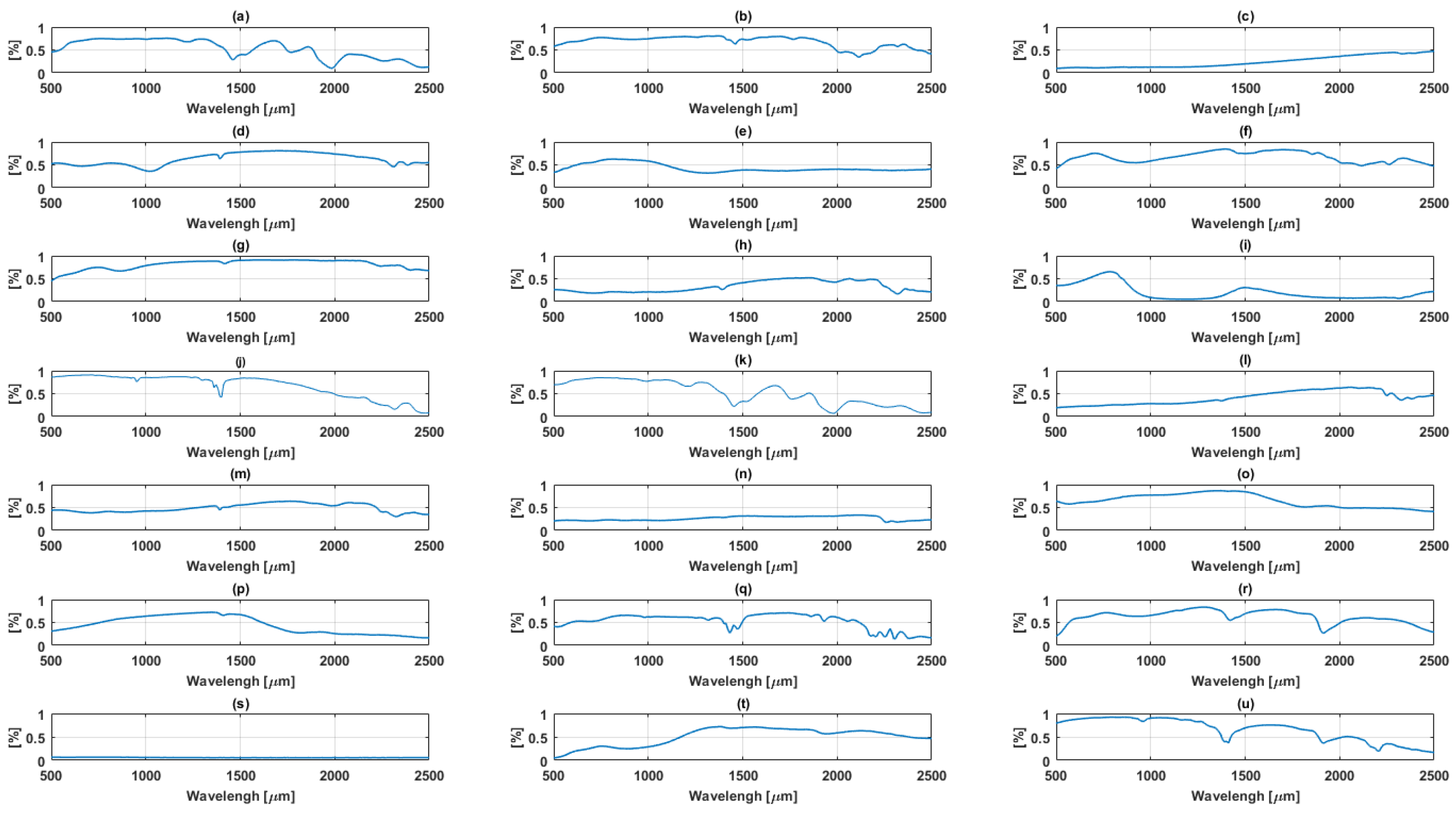
A simulated dataset of images of size pixels and 224 channels was generated with abundances computed according to a Dirichlet distribution with 21 endmembers. The spectral signatures of the endmembers are mineral reflectance with 224 bands from the ENVI spectral library [15]. Additionally, a nonlinearity co-efficient was added ranging between these parameters were tuned accordingly with different numbers of endmembers ranging from 3 to 9. The images were corrupted with Random Gaussian noise with Signal to Noise Ratio (SNR) 10 dB, 30 dB and 50 dB respectively. Figure 1 show the spectral reflectance of endmembers of the simulated data.
3.1.2. Real data
Samson Data
Samson data is a hyperspectral data owned by Oregon State University provided by WeoGeo [71], which is a push broom visible to near infrared sensor. The pixel responses are captured by 156 bands in the spectral range of 401 nm–889 nm with resolution up to nm. The data has 952 scan lines with 952 pixels in each line. For this experiment a subset of the image covering pixels was used, which is comprised of three endmembers i.e., soil, tree and water. Figure 2 shows the spectral reflectance of endmembers of the Samson data.
Jasper Ridge
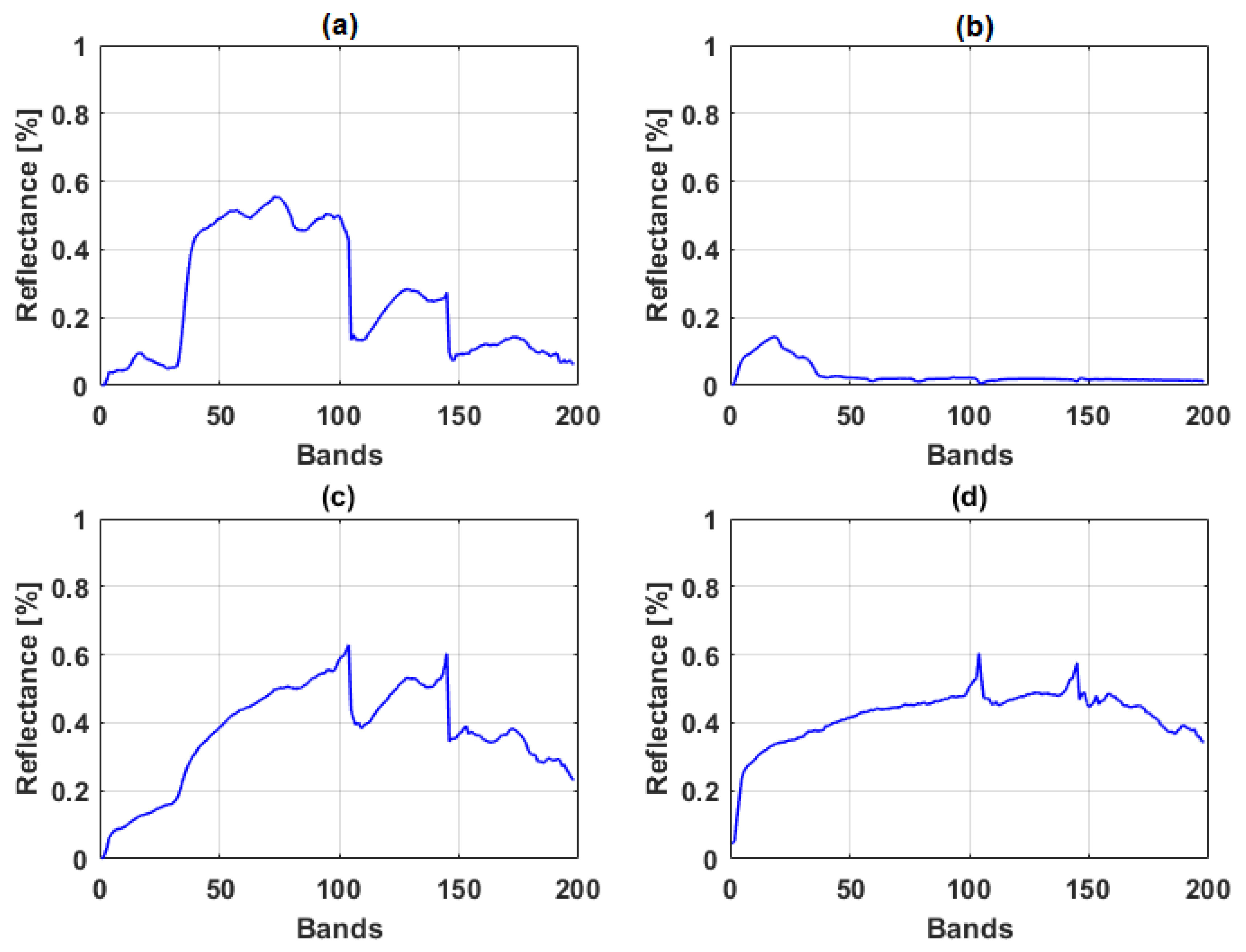
Jasper Ridge is a hyperspectral data cube recorded by AVIRIS over the standard scene of the Jasper Ridge, a biological reserve in California. The dataset consist of pixels recorded in 224 channels ranging from 380 nm to 2500 nm. The data has a spectral resolution of 9.46 nm. In this experiment, a subset of pixels was used from the original image and 198 bands were selected after removing those bands with atmospheric effects and dense water vapor. There are four main endmembers in this image: road, soil, water and tree [71]. Both datasets and corresponding abundance ground truth are available at [71], and are used as a benchmark to test classification and unmixing algorithms. Figure 3 show the spectral reflectance of endmembers of the Jasper Ridge data.
3.2. Experiments with Synthetic Data
This experiment was carried out using the synthetic dataset described in Section 3.1.1, which allows a priori control of the data. Here, VCA, FCLS, PPNMM and GBM methods were used to unmix spectra of mineral mixtures. We compared the accuracy of the individual methods to the proposed hybrid methods for switching between linear and nonlinear spectral unmixing based on the diversity of the neighboring pixels. The algorithms were coded according to [15,21,57,58]. The hybrid methods for switching were between VCA–PPNMM, VCA–GBM, FCLS–PPNMM, and FCLS–GBM, respectively. VCA was used to estimate the endmembers as contained in the dataset, while the four methods as well as the hybrid methods were used to estimate the fractional abundances. The experiment was conducted with different numbers of endmembers ranging 3, 5, 7 and 9 and different Signal to Noise Ratios of 10 dB, 30 dB and 50 dB respectively on the simulated dataset. We ran Monte Carlo simulations based on 100 generated images for each experiment.
The switching was predicted using Artificial Neural Networks (ANN). Here, we randomly split the samples into training, validation and test sets. During training, 70% of the datasets were selected to train the network, 15% were used as validation set to learn the hyperparameters of the neural networks and 15% of the remaining samples were used to test the accuracy of the networks.
In the first experiment, a window was used around the pixel of interest. A vector containing 12 values i.e., SAD min, SAD max, covariance matrix (9 values) and nonlinearity was computed for each pixel as input to train the ANN. Each input data consisted of 12 nodes with the number of hidden nodes set to 10 and the output layer having 1 node which output (0 or 1) corresponding to either a linear or nonlinear approach where a threshold was set at 0.5 for the switching. The Artificial Neural Network was used to choose between a linear or nonlinear approach for each pixel. The overall accuracy and the abundance estimation error of the methods were computed and summarized in Table 1. Results shows that the VCA – PPNMM hybrid method predicted better overall accuracy of as estimated by the confusion matrix with neural networks in switching between linear and nonlinear spectral unmixing, followed by FCLS–PPNMM with an overall accuracy of , VCA–GBM and FCLS–GBM both have an overall accuracy of and respectively. Examples showing the generated data and the error in abudance estimation are shown in Figure 4 and Figure 5. Here have chosen to display a linear method (VCA) and a non linear (GBM) for comaprison purposes and two different signal to noise ratios (SNR=10 and 50, respectively).
A second experiment was conducted with the window where each of the parameters used in creating the input training data was excluded one at a time. This was performed in order to assess the importance of the parameters in the vector created. The experiment was also repeated for SNR values 10 dB, 30 dB, and 50 dB with different endmembers of 3, 5, 7 and 9 respectively. Here we expect to have higher error values when each of the parameters are removed from the vector in comparison with the results in Table 1 where all the parameters are involved in the experiment. Results (Table 2) show that all parameters play an important role in the vector and hybrid switch methods. SAD max proves to be the most important parameter with the highest error value in the experiment where it was excluded for all SNR values as compared to the other parameters. For comparison purpose, the size of the window was increased to and the experiment repeated to evaluate the accuracy of the parameters. Results show an increase in the error value when each of the parameters is excluded from the ANN input data.
In order to assess the accuracy of the methods, we also trained a network with the raw data (i.e., 224 bands) as input instead of the vicinity parameters. Here we have 224 while the rest of the parameters remain the same. Table 3 summarizes the results of 100 Monte Carlo simulations. It is noted that the results are of the same order of magnitude as obtained in Table 1. Figure 3 displays the abundance estimated error by the 4 methods with SNR = 10 dB.
From the experiments conducted between the window and the raw data, it can be seen that the results are similar between the Signal to Noise Ratios 10 dB and 50 dB. However, the results were better with the window with a Signal to Noise Ratio of 30 dB. Therefore, it can be concluded that the ANN does not require the whole raw data and the reduced choosen parameters provide good results. Figure 5 shows the abundance results with simulated data (SNR = 50 dB). The first row shows the ground truth abundances in grayscale where a white pixel means abundance equal to one for that class and a black pixel means no abundance for that class. The other rows display the error in abundance estimation for each class and each method also coded in grayscale where the brighter the pixel, the higher the error is.
3.3. Experiment with Real Data
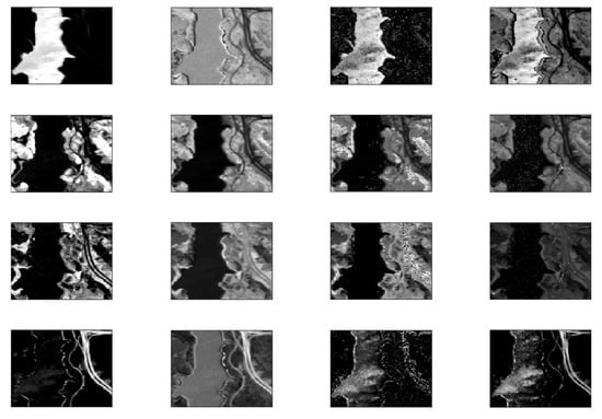
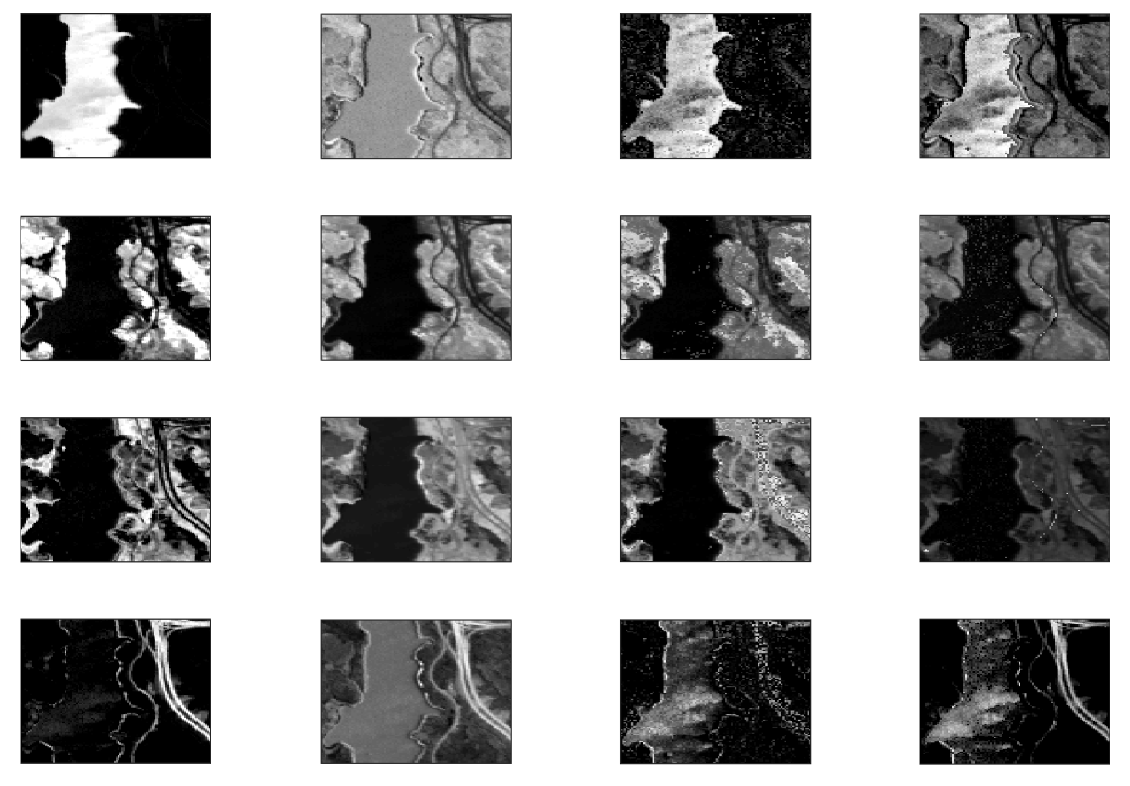
To evaluate the accuracy of the methods involved, the raw data, as well as the vicinity parameters computed in a window, and window respectively, were used to train the neural network. In the first experiment, the Jasper Ridge data was used. The training samples for each experiment were selected randomly, 70% of the samples were used for training (7000 samples), 15% each were considered for validation and testing (1500 samples for validation and 1500 samples for testing) of the neural networks. In a second experiment, the number of training samples were reduced, with 30% used for training (3000 samples), 35% each used for validation and testing (3500 samples for validation and testing) of the neural networks respectively. Finally, the experiment was repeated with 1000 and 300 training samples, respectively. Figure 6 shows the groundtruth abundances and the abundances as estimated by a linear (VCA), nonlinear (PPMM) and the corresponding hybrid methods on the Jasper Ridge data.
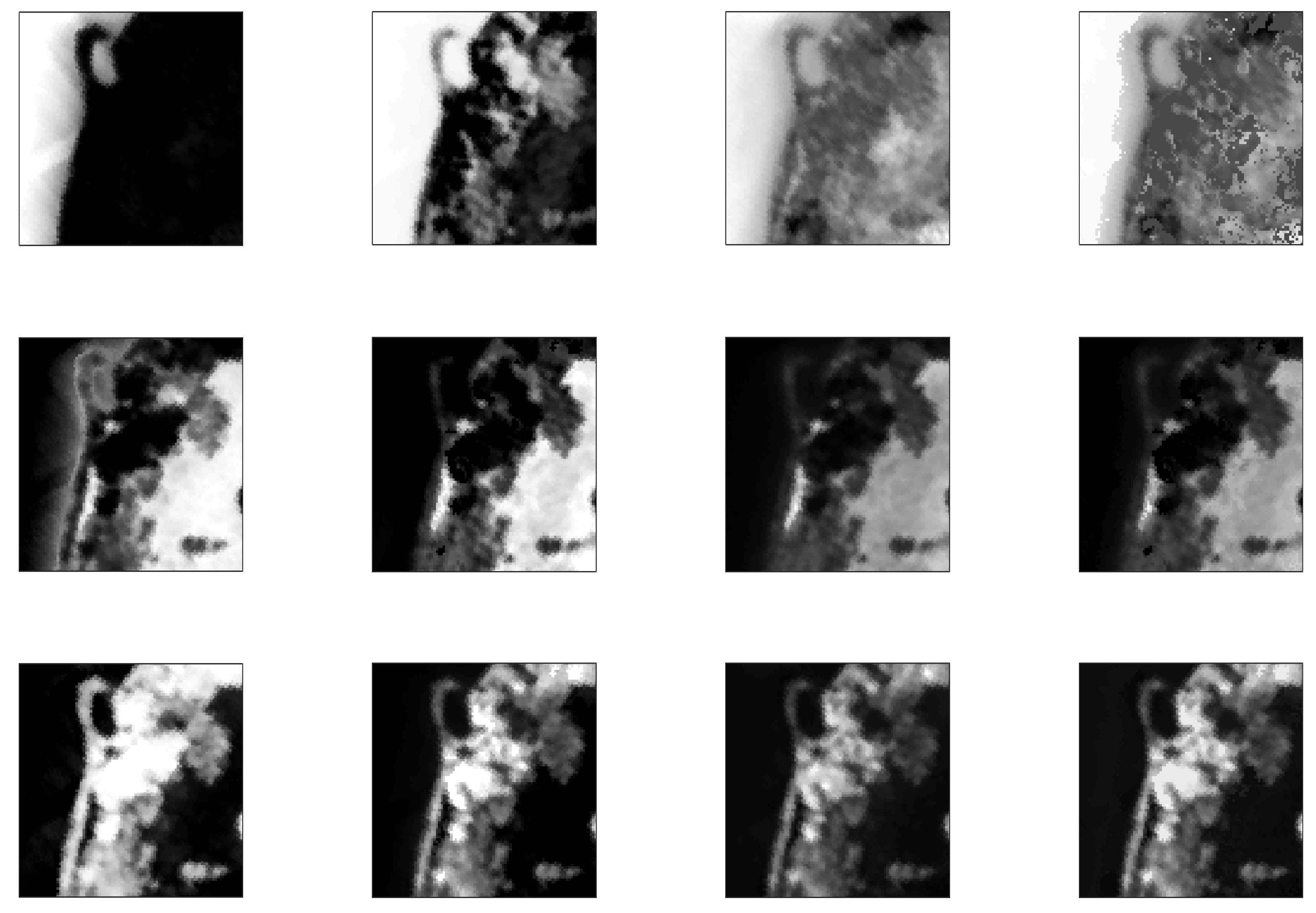
The next experiment was with Samson data, where the training, validation and testing samples were randomly selected at 70%, 15% and 15% respectively resulting in 6317 samples for training, 1353 samples each for testing and validation, then number of training samples were reduced to 30%; 35% for validation and 35% for testing which is equivalent to 2707 samples for training, 3158 samples each for validation and testing the neural networks respectively. Finally, the experiment was repeated with 1000 and 300 training samples, respectively. Figure 7 shows the groundtruth abundances, and the abundances as estimated by the a linear (VCA), nonlinear (PPMM) and hybrid methods on the Samson data.
The experiment was repeated on a window, and window. This was to compare and evaluate the accuracy of the hybrid methods with regards to the size of the data used to train the networks. The results on both datasets show that our proposed methods achieved the best results in all scenarios. Results of the experiments based on the abundance estimation error, are summarized in Table 4 and Table 5.
The overall accuracy of the network, the abundance estimation error, the training, validation and testing abundance error of the networks were used to evaluate the performance of the methods investigated in this paper. From the results obtained, experiments with the raw dataset, and windows produce similar overall accuracy in all the experiments. It indicates that the hybrid methods for switching between linear and nonlinear spectral unmixing are more effective than the individual methods, meanwhile, it can also be said that ANN pattern recognition has good capability in recognizing patterns which is very effective even with fewer samples used to train the network. From the four hybrid switch methods, the VCA – PPNMM method outperforms the other methods with a higher overall accuracy of 96% as compared to the other methods, FCLS – PPNMM has an overall accuracy of 94.5% while VCA – GBM and FCLS – GBM both have overall accuracies of 92.8%. VCA – PPNMM also has the lowest abundance estimation error and produced the lowest abundance error in terms of training, validation and testing of the neural networks. However, it can be observed that the proposed hybrid switch methods obtained similar results when using the and window to conduct the experiment when fewer samples were used to train the networks. Therefore, it shows that the proposed hybrid method does not requires all the raw data for training the networks and can be used effectively to switch between linear and nonlinear spectral unmixing of hyperspectral data. In terms of computational time, the individual methods are 40% more time consuming compared to the hybrid method thereby making them computationally expensive in terms of simulation. Table 6 and Table 7 summarizes the result of the experiments showing the accuracy of the neural network based on training, testing and validation of the networks.
4. Discussion
4.1. Results
Nonlinearity occurs when the photons interact with different materials before reaching the sensor. We assumed here that the linear mixing could be associated to mixtures for which the pixel components appear in spatially segregated patterns. More specifically areas that are spatially correlated are more likely to be explained with the linear model. In this paper, we first used controlled simulated data. Each image consisted of a series of regions. Each region had the same type of ground cover with added noise. Figure 5 shows the results for the simulated data with 5 classes and SNR = 50 dB. Although the average error is in the same order of magnitude for both linear and nonlinear approaches, the distribution of the error differs. It is noted that the linear model (VCA) detects well the low abundances of classes and pixels that do not contain a particular class (shown in black in the ground truth figures). The errors are related to quantification rather than to detecting the wrong class. This might be due to the algorithm performing worse with high spectral variability within the classes. The non-linear method (GBM), on the other hand, returns an error which is more uniform and not so related to the spatial pattern of the data or spectral variability as displayed in Figure 4 and Figure 5. The proposed approach assumptions are further proven with the real data sets. In particular, the Jasper Ridge data set includes different classes; water, soil and road. Figure 6 shows the abundance estimation for the different methods. It is noted that VCA has been reported to underperform in this data set [27]. However, the road class is very well identified against the non-linear methods that failed to detect this class. On the other hand, the linear methods failed to classify correctly the water class which is more spectrally variable medium. Thus, it seems that noise and endmember spectral variability makes the non-linear models outperforming the linear ones while the spatially structured areas are well defined with the linear model. The vicinity parameters used in this paper address both the spatial and spectral diversity of the data. The test shown in Table 2 showed that all parameters played an important role in the decision making process. Moreover, Figure 6 and Figure 7 also support that the chosen features are suitable and that the switching is appropriate achieving improved results.
4.2. Advantages and Limitations
The proposed method provides a switch between unmixing methods for given spectral images. It can not only provide more accurate results, as shown in the experimental section but also reduce computational costs by selecting the most appropriate approach. This research study has proven the capabilities of the proposed methodology based on certain parameters. However, the supervised ANN relies on having ground truth data for training which is not always available. Future work will expand to unsupervised approaches such as self-organizing maps which have been successfully used in spectral data for classification and anomaly detection tasks [33,72]. Although we used spatial and spectral features within windows for learning and thus to make the decision, the switching was made at individual pixel level. Thus future work will base the decision on group of pixels or areas using for instance Markov random fields.
5. Conclusions
In this paper, a new hybrid switch method for switching between linear and nonlinear spectral unmixing of hyperspectral data based on deep learning neural networks is proposed. The endmembers were extracted using VCA while the abundances were estimated using individual and hybrid methods. The ANN was trained with a set of parameters extracted from the diversity of the neighboring pixels of the images computed within a and window. These parameters are spectral angular distance, covariance and nonlinearity parameters. Experiments were conducted with different Signal to Noise Ratio (SNR) ranging between 10 dB, 30 dB, 50 dB and different numbers of endmembers: 3, 5, 7 and 9. We have noted that the hybrid methods are more suitable than the individual technique with high overall accuracy and the abundance estimation error is significantly lower than that obtained with the individual methods in particular, VCA – PPNMM proved to be the best with about 98% accuracy in all the experiments conducted. The experiment with the Jasper Ridge and Samson data confirmed the effectiveness of the approach. The method was applied to two real datasets with ANN trained using 70%, , and samples. Experimentation with the real data, window and window vectors, proved the effectiveness of the hybrid switch methods, the results show that the size of datasets used for training the network and the vector size does not affect the accuracy of the hybrid methods in switching between linear and nonlinear spectral unmixing, which means that the network can be trained with less sample data without the loss of prediction accuracy. An area to consider for future research is the application of Markovian Jump method for switching between linear/nonlinear spectral unmixing.
Acknowledgments
The authors will like to acknowledge Tertiary Education Trust Fund (TETFUND) and Kaduna State University, Nigeria for providing the funds to support this PhD and to Kingston University which covers the cost to publish in open source journals.
Author Contributions
All authors have made great contributions to the work. Asmau Ahmed and Olga Duran conceived and designed the experiments, Asmau Ahmed, Olga Duran, Yahya Zweiri and Mike Smith analyzed the data and revised the manuscript.
Conflicts of Interest
The authors declare no conflict of interest.The funding sponsors had no role in the design of the study; in the collection, analyses, or interpretation of data; in the writing of the manuscript, and in the decision to publish the results.
References
- Keshava, N.; Mustard, J.F. Spectral unmixing. IEEE Signal Process. Mag. 2002, 19, 44–57. [Google Scholar] [CrossRef]
- Xu, M.; Zhang, L.; Du, B.; Zhang, L.; Fan, Y.; Song, D. A Mutation Operator Accelerated Quantum-Behaved Particle Swarm Optimization Algorithm for Hyperspectral Endmember Extraction. Remote Sens. 2017, 9, 197. [Google Scholar] [CrossRef]
- Uezato, T.; Murphy, R.J.; Melkumyan, A.; Chlingaryan, A. A novel spectral unmixing method incorporating spectral variability within endmember classes. IEEE Trans. Geosci. Remote Sens. 2016, 54, 2812–2831. [Google Scholar] [CrossRef]
- Weeks, A.R. Fundamentals of Electronic Image Processing; SPIE Optical Engineering Press: Bellingham, WA, USA, 1996. [Google Scholar]
- Drumetz, L.; Tochon, G.; Chanussot, J.; Jutten, C. Estimating the number of endmembers to use in spectral unmixing of hyperspectral data with collaborative sparsity. In Proceedings of the the 13th International Conference on Latent Variable Analysis and Signal Separation (LVA-ICA), Grenoble, France, 21–23 February 2017; pp. 1–10. [Google Scholar]
- Hapke, B. Bidirectional reflectance spectroscopy: 1. Theory. J. Geophys. Res. 1981, 86, 3039–3054. [Google Scholar] [CrossRef]
- Dobigeon, N.; Tourneret, J.Y.; Richard, C.; Bermudez, J.; McLaughlin, S.; Hero, A.O. Nonlinear unmixing of hyperspectral images: Models and algorithms. IEEE Signal Process. Mag. 2014, 31, 82–94. [Google Scholar] [CrossRef]
- Halimi, A.; Altmann, Y.; Buller, G.S.; McLaughlin, S.; Oxford, W.; Clarke, D.; Piper, J. Robust unmixing algorithms for hyperspectral imagery. In Proceedings of the Sensor Signal Processing for Defence (SSPD), Edinburgh, UK, 22–23 September 2016; pp. 1–5. [Google Scholar]
- Chang, C.I. Adaptive Linear Spectral Mixture Analysis. IEEE Trans. Geosci. Remote Sens. 2017, 55, 1240–1253. [Google Scholar]
- Shi, Z.; Tang, W.; Duren, Z.; Jiang, Z. Subspace matching pursuit for sparse unmixing of hyperspectral data. IEEE Trans. Geosci. Remote Sens. 2014, 52, 3256–3274. [Google Scholar]
- Iordache, M.D.; Bioucas-Dias, J.M.; Plaza, A. Sparse unmixing of hyperspectral data. IEEE Trans. Geosci. Remote Sens. 2011, 49, 2014–2039. [Google Scholar]
- Li, C.; Ma, Y.; Mei, X.; Liu, C.; Ma, J. Hyperspectral unmixing with robust collaborative sparse regression. Remote Sens. 2016, 8, 588. [Google Scholar]
- Thouvenin, P.A.; Dobigeon, N.; Tourneret, J.Y. Hyperspectral unmixing with spectral variability using a perturbed linear mixing model. IEEE Trans. Signal Process. 2016, 64, 525–538. [Google Scholar]
- Foody, G.M.; Cox, D. Subpixel Land Cover Composition Estimation Using Linear Mixture Model and Fuzzy Membership Functions. Int. J. Remote Sens. 1994, 15, 619–631. [Google Scholar] [CrossRef]
- Nascimento, J.M.; Dias, J.M.B. Vertex component analysis: A fast algorithm to unmix hyperspectral data. IEEE Trans. Geosci. Remote Sens. 2005, 43, 898–910. [Google Scholar] [CrossRef]
- Nascimento, J.M.; Bioucas-Dias, J.M. Nonlinear mixture model for hyperspectral unmixing. In Proceedings of the SPIE Europe Remote Sensing. International Society for Optics and Photonics, Berlin, Germany, 31 August 2009; p. 74770I. [Google Scholar]
- Li, C.; Ma, Y.; Huang, J.; Mei, X.; Liu, C.; Ma, J. GBM-based unmixing of hyperspectral data using bound projected optimal gradient method. IEEE Geosci. Remote Sens. Lett. 2016, 13, 952–956. [Google Scholar] [CrossRef]
- Chen, J.; Richard, C.; Honeine, P. Nonlinear unmixing of hyperspectral data based on a linear-mixture/nonlinear-fluctuation model. IEEE Trans. Signal Process. 2013, 61, 480–492. [Google Scholar] [CrossRef]
- Marinoni, A.; Gamba, P. Accurate detection of anthropogenic settlements in hyperspectral images by higher order nonlinear unmixing. IEEE J. Sel. Top. Appl. Earth Obs. Remote Sens. 2016, 9, 1792–1801. [Google Scholar] [CrossRef]
- Altmann, Y. Nonlinear Spectral Unmixing of Hyperspectral Images. Ph.D. Thesis, l’Institut National Polytechnique de Toulouse (INP Toulouse), Toulouse, France, 2013. [Google Scholar]
- Altmann, Y.; Halimi, A.; Dobigeon, N.; Tourneret, J.Y. Supervised nonlinear spectral unmixing using a postnonlinear mixing model for hyperspectral imagery. IEEE Trans. Image Process. 2012, 21, 3017–3025. [Google Scholar] [CrossRef] [PubMed] [Green Version]
- Nascimento, J.M.; Bioucas-Dias, J.M. Unmixing hyperspectral intimate mixtures. In Proceedings of the Remote Sensing. International Society for Optics and Photonics, Toulouse, France, 20 September 2010; p. 78300C. [Google Scholar]
- Sun, L.; Wu, Z.; Liu, J.; Xiao, L.; Wei, Z. Supervised spectral–spatial hyperspectral image classification with weighted Markov random fields. IEEE Trans. Geosci. Remote Sens. 2015, 53, 1490–1503. [Google Scholar] [CrossRef]
- Fauvel, M.; Benediktsson, J.A.; Chanussot, J.; Sveinsson, J.R. Spectral and spatial classification of hyperspectral data using SVMs and morphological profiles. IEEE Trans. Geosci. Remote Sens. 2008, 46, 3804–3814. [Google Scholar] [CrossRef]
- Yu, H.; Gao, L.; Li, J.; Li, S.S.; Zhang, B.; Benediktsson, J.A. Spectral-spatial hyperspectral image classification using subspace-based support vector machines and adaptive markov random fields. Remote Sens. 2016, 8, 355. [Google Scholar] [CrossRef]
- Ni, L.; Gao, L.; Li, S.; Li, J.; Zhang, B. Edge-constrained Markov random field classification by integrating hyperspectral image with LiDAR data over urban areas. J. Appl. Remote Sens. 2014, 8, 085089. [Google Scholar] [CrossRef]
- Zhang, B.; Li, S.; Jia, X.; Gao, L.; Peng, M. Adaptive Markov random field approach for classification of hyperspectral imagery. IEEE Geosci. Remote Sens. Lett. 2011, 8, 973–977. [Google Scholar] [CrossRef]
- Jimenez, L.O.; Landgrebe, D.A. Supervised classification in high-dimensional space: Geometrical, statistical, and asymptotical properties of multivariate data. IEEE Trans. Syst. Man Cybern. Part C 1998, 28, 39–54. [Google Scholar] [CrossRef]
- Martínez, P.; Gualtieri, J.; Aguilar, P.; Pérez, R.; Linaje, M.; Preciado, J.; Plaza, A. Hyperspectral Image Classification Using a Self-organizing Map. Available online: http://www.umbc.edu/rssipl/people/aplaza/Papers/Conferences/2001.AVIRIS.SOM.pdf (accessed on 1 June 2017).
- Fauvel, M.; Tarabalka, Y.; Benediktsson, J.A.; Chanussot, J.; Tilton, J.C. Advances in spectral-spatial classification of hyperspectral images. Proc. IEEE 2013, 101, 652–675. [Google Scholar] [CrossRef]
- Raith, S.; Vogel, E.P.; Anees, N.; Keul, C.; Güth, J.F.; Edelhoff, D.; Fischer, H. Artificial Neural Networks as a powerful numerical tool to classify specific features of a tooth based on 3D scan data. Comput. Biol. Med. 2017, 80, 65–76. [Google Scholar] [CrossRef] [PubMed]
- Han, T.; Jiang, D.; Zhao, Q.; Wang, L.; Yin, K. Comparison of random forest, artificial neural networks and support vector machine for intelligent diagnosis of rotating machinery. Trans. Inst. Meas. Control 2017. [Google Scholar] [CrossRef]
- Pal, S.K.; Mitra, S. Multilayer perceptron, fuzzy sets, and classification. IEEE Trans. Neural Netw. 1992, 3, 683–697. [Google Scholar] [CrossRef] [PubMed]
- Duran, O.; Althoefer, K.; Seneviratne, L.D. Automated pipe defect detection and categorization using camera/laser-based profiler and artificial neural network. IEEE Trans. Autom. Sci. Eng. 2007, 4, 118–126. [Google Scholar] [CrossRef]
- Li, Y.; Zhang, H.; Shen, Q. Spectral–Spatial Classification of Hyperspectral Imagery with 3D Convolutional Neural Network. Remote Sens. 2017, 9, 67. [Google Scholar] [CrossRef]
- Duran, O.; Petrou, M. A time-efficient clustering method for pure class selection. In Proceedings of the 2005 IEEE International Geoscience and Remote Sensing Symposium (IGARSS’05), Seoul, Korea, 29 July 2005; Volume 1. [Google Scholar] [CrossRef]
- Pérez-Hoyos, A.; Martínez, B.; García-Haro, F.J.; Moreno, Á.; Gilabert, M.A. Identification of ecosystem functional types from coarse resolution imagery using a self-organizing map approach: A case study for Spain. Remote Sens. 2014, 6, 11391–11419. [Google Scholar] [CrossRef]
- Penn, B.S. Using self-organizing maps to visualize high-dimensional data. Comput. Geosci. 2005, 31, 531–544. [Google Scholar] [CrossRef]
- Wei, Y.; Qiu, J.; Shi, P.; Lam, H.K. A new design of H-infinity piecewise filtering for discrete-time nonlinear time-varying delay systems via TS fuzzy affine models. IEEE Trans. Syst. Man Cybern. 2017. [Google Scholar] [CrossRef]
- Wei, Y.; Qiu, J.; Lam, H.K.; Wu, L. Approaches to TS fuzzy-affine-model-based reliable output feedback control for nonlinear Itô stochastic systems. IEEE Trans. Fuzzy Syst. 2016. [Google Scholar] [CrossRef]
- Lam, H.K.; Li, H.; Liu, H. Stability analysis and control synthesis for fuzzy-observer-based controller of nonlinear systems: A fuzzy-model-based control approach. IET Control Theory Appl. 2013, 7, 663–672. [Google Scholar] [CrossRef]
- Wei, Y.; Qiu, J.; Karimi, H.R.; Wang, M. Model reduction for continuous-time Markovian jump systems with incomplete statistics of mode information. Int. J. Syst. Sci. 2014, 45, 1496–1507. [Google Scholar] [CrossRef]
- Wang, H.; Shi, P.; Agarwal, R.K. Network-based event-triggered filtering for Markovian jump systems. Int. J. Control 2016, 89, 1096–1110. [Google Scholar] [CrossRef]
- Chen, Y.; Lin, Z.; Zhao, X.; Wang, G.; Gu, Y. Deep learning-based classification of hyperspectral data. IEEE J. Sel. Top. Appl. Earth Obs. Remote Sens. 2014, 7, 2094–2107. [Google Scholar] [CrossRef]
- Audebert, N.; Saux, B.L.; Lefèvre, S. Segment-before-Detect: Vehicle Detection and Classification through Semantic Segmentation of Aerial Images. Remote Sens. 2017, 9, 368. [Google Scholar] [CrossRef]
- Ammour, N.; Alhichri, H.; Bazi, Y.; Benjdira, B.; Alajlan, N.; Zuair, M. Deep Learning Approach for Car Detection in UAV Imagery. Remote Sens. 2017, 9, 312. [Google Scholar] [CrossRef]
- Bejiga, M.B.; Zeggada, A.; Nouffidj, A.; Melgani, F. A convolutional neural network approach for assisting avalanche search and rescue operations with uav imagery. Remote Sens. 2017, 9, 100. [Google Scholar] [CrossRef]
- Lyu, H.; Lu, H.; Mou, L. Learning a Transferable Change Rule from a Recurrent Neural Network for Land Cover Change Detection. Remote Sens. 2016, 8, 506. [Google Scholar] [CrossRef]
- Makantasis, K.; Karantzalos, K.; Doulamis, A.; Doulamis, N. Deep supervised learning for hyperspectral data classification through convolutional neural networks. In Proceedings of the 2015 IEEE International Geoscience and Remote Sensing Symposium (IGARSS 2015), Milan, Italy, 26–31 July 2015; pp. 4959–4962. [Google Scholar]
- Giorgio, L.; Frate, F.D. A Neural Network Approach for Pixel Unmixing in Hyperspectral Data; Earth Observation Laboratory- Tor Vergata University Via del Politecnico: Rome, Italy.
- Kumar, U.; Raja, K.S.; Mukhopadhyay, C.; Ramachandra, T.V. A Neural Network Based Hybrid Mixture Model to Extract Information from Nonlinear Mixed Pixels. Information 2012, 3, 420–441. [Google Scholar] [CrossRef]
- Giorgio, A.L.; Frate, F.D. Pixel Unmixing in Hyperspectral Data by Means of Neural Networks. IEEE Trans. Geosci. Remote Sens. 2011, 49, 4163–4172. [Google Scholar]
- Wu, H.; Prasad, S. Convolutional Recurrent Neural Networks forHyperspectral Data Classification. Remote Sens. 2017, 9, 298. [Google Scholar] [CrossRef]
- Atkinson, P.M.; Cutler, M.E.J.; Lewis, H. Mapping Sub-Pixel Proportional Land Cover With AVHRR Imagery. Int. J. Remote Sens. 1997, 18, 917–935. [Google Scholar] [CrossRef]
- Somers, B.; Asner, G.P.; Tits, L.; Coppin, P. Endmember variability in spectral mixture analysis: A review. Remote Sens. Environ. 2011, 115, 1603–1616. [Google Scholar] [CrossRef]
- Somers, B.; Cools, K.; Delalieux, S.; Stuckens, J.; Van der Zande, D.; Verstraeten, W.W.; Coppin, P. Nonlinear hyperspectral mixture analysis for tree cover estimates in orchards. Remote Sens. Environ. 2009, 113, 1183–1193. [Google Scholar] [CrossRef]
- Heinz, D.C.; Chang, C.-I. Fully constrained least squares linear spectral mixture analysis method for material quantification in hyperspectral imagery. IEEE Trans. Geosci. Remote Sens. 2001, 39, 529–545. [Google Scholar] [CrossRef]
- Altmann, Y.; Dobigeon, N.; Tourneret, J.Y. Bilinear models for nonlinear unmixing of hyperspectral images. In Proceedings of the 2011 3rd Workshop on Hyperspectral Image and Signal Processing: Evolution in Remote Sensing (WHISPERS), Lisbon, Portugal, 6–9 June 2011; pp. 1–4. [Google Scholar]
- Nascimento, J.M.; Dias, J.M.B. Does independent component analysis play a role in unmixing hyperspectral data? IEEE Trans. Geosci. Remote Sens. 2005, 43, 175–187. [Google Scholar] [CrossRef]
- Bioucas-Dias, J.M.; Plaza, A.; Dobigeon, N.; Parente, M.; Du, Q.; Gader, P.; Chanussot, J. Hyperspectral unmixing overview: Geometrical, statistical, and sparse regression-based approaches. IEEE J. Sel. Top. Appl. Earth Obs. Remote Sens. 2012, 5, 354–379. [Google Scholar] [CrossRef]
- Halimi, A.; Altmann, Y.; Dobigeon, N.; Tourneret, J.Y. Nonlinear unmixing of hyperspectral images using a generalized bilinear model. IEEE Trans. Geosci. Remote Sens. 2011, 49, 4153–4162. [Google Scholar] [CrossRef] [Green Version]
- Altmann, Y.; Pereyra, M.; McLaughlin, S. Bayesian nonlinear hyperspectral unmixing with spatial residual component analysis. IEEE Trans. Comput. Imaging 2015, 1, 174–185. [Google Scholar] [CrossRef]
- Sohn, Y.; McCoy, R.M. Mapping desert shrub rangeland using spectral unmixing and modeling spectral mixtures with TM data. Photogramm. Eng. Remote Sens. 1997, 63, 707–716. [Google Scholar]
- Tuzel, O.; Porikli, F.; Meer, P. Region covariance: A fast descriptor for detection and classification. In Proceedings of the European Conference on Computer Vision, Graz, Austria, 7–13 May 2006; Springer: Berlin/Heidelberg, Germany, 2006; pp. 589–600. [Google Scholar]
- Ripley, B.D. Pattern Recognition and Neural Networks; Cambridge University Press: Cambridge, UK, 2007. [Google Scholar]
- Charalambous, C. Conjugate gradient algorithm for efficient training of artificial neural networks. IEEE Proc. G 1992, 139, 301–310. [Google Scholar] [CrossRef]
- Saini, L.M.; Soni, M.K. Artificial neural network-based peak load forecasting using conjugate gradient methods. IEEE Trans. Power Syst. 2002, 17, 907–912. [Google Scholar] [CrossRef]
- Nabipour, M.; Keshavarz, P. Modeling surface tension of pure refrigerants using feed-forward back-propagation neural networks. Int. J. Refrig. 2017, 75, 217–227. [Google Scholar] [CrossRef]
- LeCun, Y.; Bengio, Y.; Hinton, G. Deep learning. Nature 2015, 521, 436–444. [Google Scholar] [CrossRef] [PubMed]
- Hu, X.; Yuan, Y. Deep-Learning-Based Classification for DTM Extraction from ALS Point Cloud. Remote Sens. 2016, 8, 730. [Google Scholar] [CrossRef]
- Zhu, F.; Wang, Y.; Fan, B.; Xiang, S.; Meng, G.; Pan, C. Spectral unmixing via data-guided sparsity. IEEE Trans. Image Process. 2014, 23, 5412–5427. [Google Scholar] [CrossRef] [PubMed]
- Duran, O.; Petrou, M. A time-efficient method for anomaly detection in hyperspectral images. IEEE Trans. Geosci. Remote Sens. 2007, 45, 3894–3904. [Google Scholar] [CrossRef]
Figure 1.
Spectral reflectance of endmembers of the simulated data plotted, reflectance [%] against wavelength (a) Brucite; (b) Clinochlore; (c) Axinite; (d) Erionite; (e) Ammonioalunite; (f) Clintonite; (g) Almandine; (h) Carnallite; (i) Actinolite; (j) Andradite; (k) Antigorite; (l) Elbaite; (m) Ammonio-jarosite; (n) Diaspore; (o) Halloysite; (p) Biotite; (q) Galena; (r) Carnallite; (s) Chlorite; (t) Goethite; (u) Corundum.

Figure 2.
Spectral reflectance of endmembers of the Samson data (a) rock; (b) tree; (c) water.
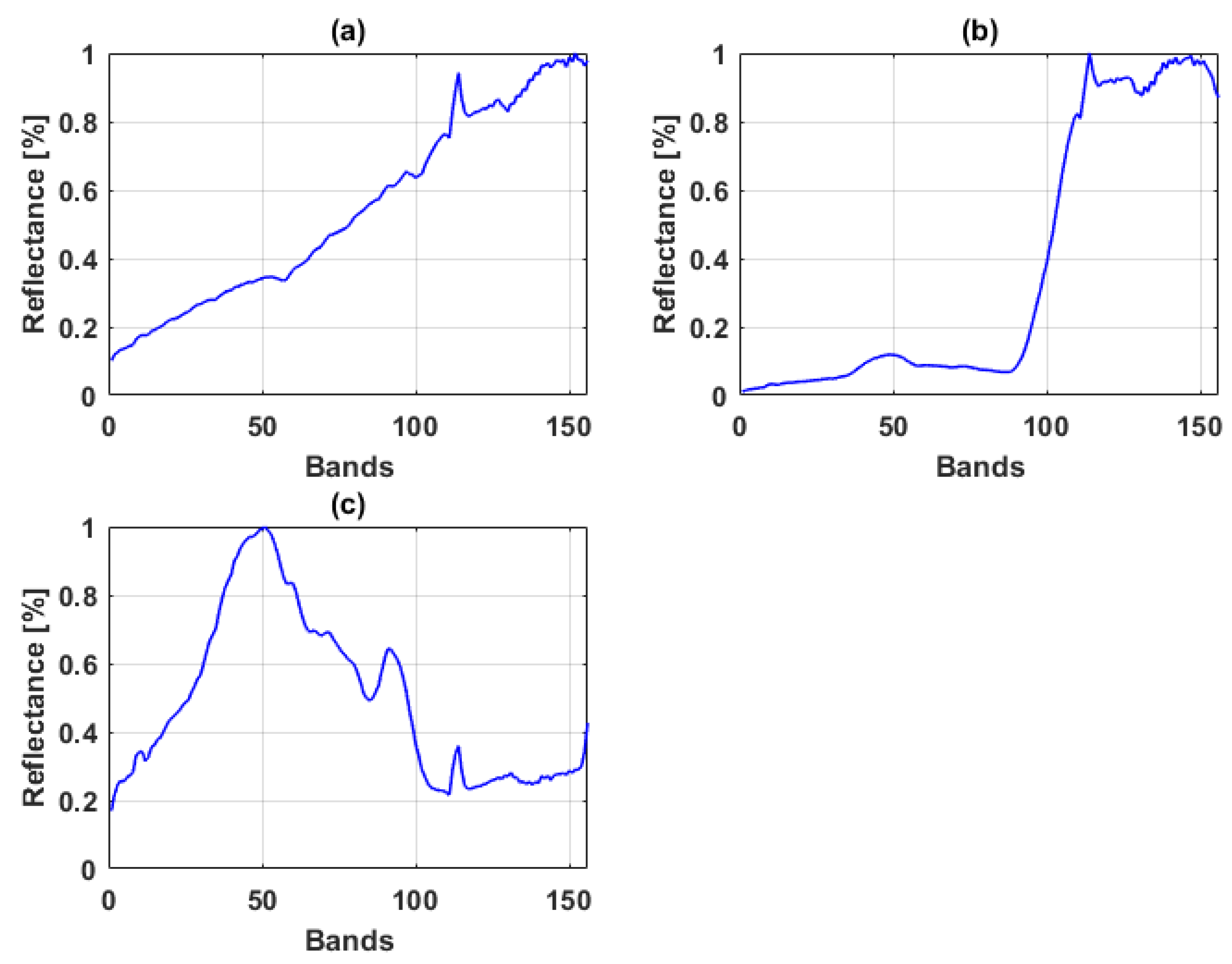
Figure 3.
Spectral reflectance of endmembers of the Jasper Ridge data (a) tree; (b) water; (c) soil; (d) road.
Figure 3.
Spectral reflectance of endmembers of the Jasper Ridge data (a) tree; (b) water; (c) soil; (d) road.

Figure 4.
Abundance estimation errors with simulated data with 5 endmembers (SNR = 10 dB). The first row shows the ground truth abundances for the 5 classes. From the top, then the error in abundances as estimated by the hybrid, VCA and GBM methods, respectively.
Figure 4.
Abundance estimation errors with simulated data with 5 endmembers (SNR = 10 dB). The first row shows the ground truth abundances for the 5 classes. From the top, then the error in abundances as estimated by the hybrid, VCA and GBM methods, respectively.
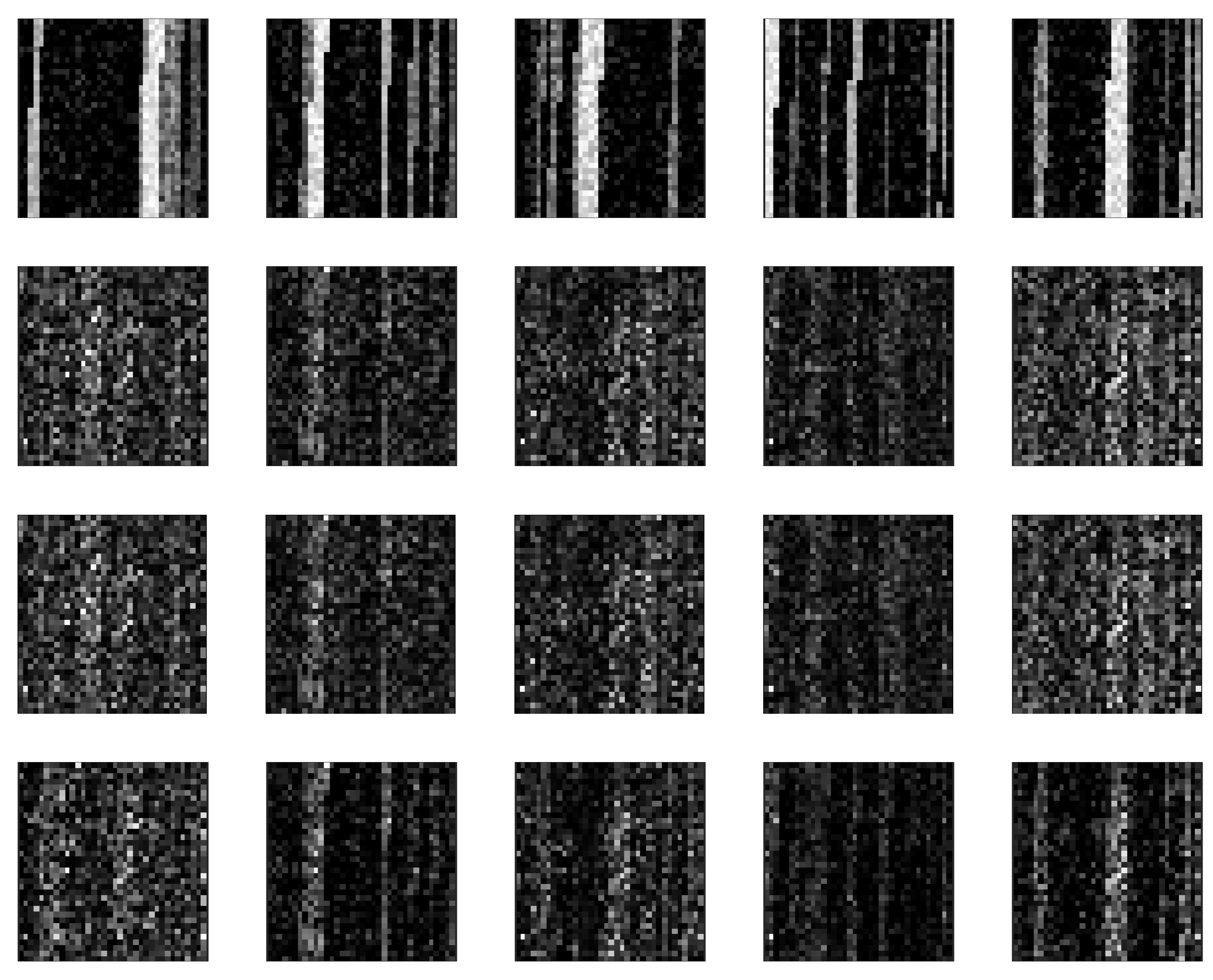
Figure 5.
Abundance estimation errors with simulated data with 5 endmembers (SNR = 50 dB). The first row shows the ground truth abundances for the 5 classes. From the top, then the error in abundances as estimated by the hybrid, VCA and GBM methods, respectively.
Figure 5.
Abundance estimation errors with simulated data with 5 endmembers (SNR = 50 dB). The first row shows the ground truth abundances for the 5 classes. From the top, then the error in abundances as estimated by the hybrid, VCA and GBM methods, respectively.
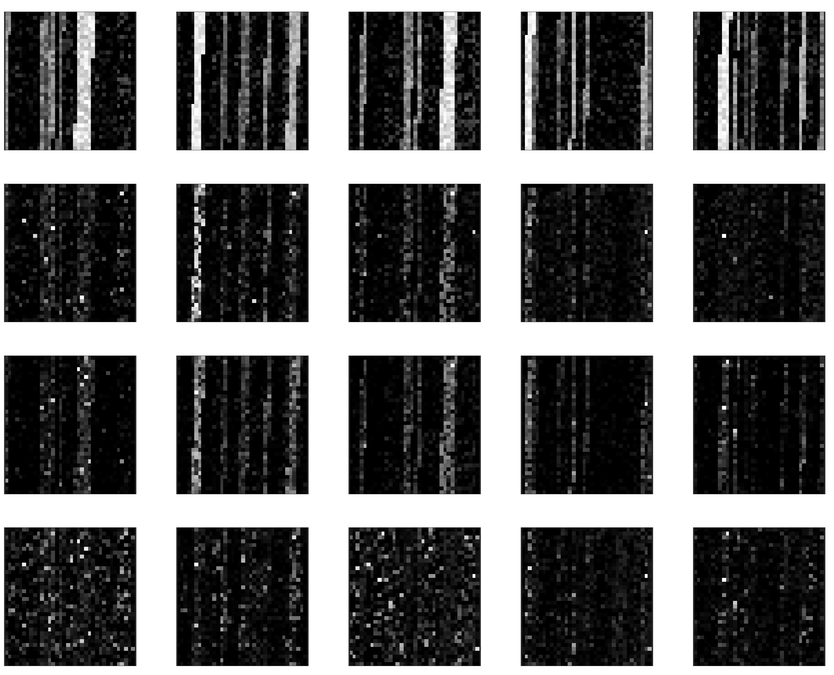
Figure 6.
Abundance estimate of endmembers of the Jasper Ridge data showing from left; the groundtruth, linear (VCA), nonlinear (PPMM) and the hybrid methods. From top water; tree; soil; and road.
Figure 6.
Abundance estimate of endmembers of the Jasper Ridge data showing from left; the groundtruth, linear (VCA), nonlinear (PPMM) and the hybrid methods. From top water; tree; soil; and road.

Figure 7.
Abundance estimate of endmembers of the Samson data showing the groundtruth, linear (VCA), nonlinear (PPMM) and the hybrid methods. From top water; rock; tree.
Figure 7.
Abundance estimate of endmembers of the Samson data showing the groundtruth, linear (VCA), nonlinear (PPMM) and the hybrid methods. From top water; rock; tree.

Table 1.
Abundance estimation error ( window )of the individual and hybrid methods between linear and nonlinear spectral unmixing with different signal to noise ratios and endmembers. The best results are shown in bold.
Table 1.
Abundance estimation error ( window )of the individual and hybrid methods between linear and nonlinear spectral unmixing with different signal to noise ratios and endmembers. The best results are shown in bold.
| SNR (dB) = 50 | ||||
|---|---|---|---|---|
| INDIVIDUAL METHODS | ||||
| PPNMM | 0.0206 | 0.0307 | 0.0371 | 0.0486 |
| GBM | 0.0207 | 0.0303 | 0.0346 | 0.0449 |
| VCA | 0.0521 | 0.0696 | 0.0777 | 0.0778 |
| FCLS | 0.0714 | 0.0916 | 0.0922 | 0.0924 |
| HYBRID METHODS | ||||
| VCA – PPNMM | 0.0117 | 0.0201 | 0.0143 | 0.0373 |
| VCA – GBM | 0.0189 | 0.0201 | 0.0158 | 0.0353 |
| FCLS – PPNMM | 0.0177 | 0.0179 | 0.0177 | 0.0340 |
| FCLS – GBM | 0.0193 | 0.0196 | 0.0199 | 0.0174 |
| SNR (dB) = 30 | ||||
| INDIVIDUAL METHODS | ||||
| PPNMM | 0.0696 | 0.0951 | 0.0914 | 0.0886 |
| GBM | 0.0965 | 0.1193 | 0.1405 | 0.1285 |
| VCA | 0.0597 | 0.0662 | 0.0886 | 0.0945 |
| FCLS | 0.0684 | 0.0747 | 0.0894 | 0.0911 |
| HYBRID METHODS | ||||
| VCA – PPNMM | 0.0390 | 0.0317 | 0.0421 | 0.0556 |
| VCA – GBM | 0.0591 | 0.0412 | 0.0579 | 0.0662 |
| FCLS – PPNMM | 0.0396 | 0.0320 | 0.0539 | 0.0645 |
| FCLS – GBM | 0.0866 | 0.0926 | 0.0990 | 0.1081 |
| SNR (dB) = 10 | ||||
| INDIVIDUAL METHODS | ||||
| PPNMM | 0.0907 | 0.1510 | 0.1640 | 0.1733 |
| GBM | 0.1106 | 0.1222 | 0.1334 | 0.1740 |
| VCA | 0.1289 | 0.1514 | 0.1257 | 0.1988 |
| FCLS | 0.1169 | 0.1702 | 0.1791 | 0.1763 |
| HYBRID METHODS | ||||
| VCA – PPNMM | 0.0401 | 0.0421 | 0.0736 | 0.0775 |
| VCA – GBM | 0.0704 | 0.0911 | 0.0813 | 0.0915 |
| FCLS – PPNMM | 0.0440 | 0.0508 | 0.0813 | 0.0814 |
| FCLS – GBM | 0.0917 | 0.0959 | 0.1099 | 0.1112 |
Table 2.
Abundance estimation error ( window) of the individual and hybrid methods between linear and nonlinear spectral unmixing with different signal to noise ratios and 3 endmembers where each of the parameters is removed one at a time. The best results are shown in bold.
Table 2.
Abundance estimation error ( window) of the individual and hybrid methods between linear and nonlinear spectral unmixing with different signal to noise ratios and 3 endmembers where each of the parameters is removed one at a time. The best results are shown in bold.
| WITHOUT SAD MIN. | SNR (dB) = 10 | SNR (dB) = 30 | SNR (dB) = 50 |
|---|---|---|---|
| INDIVIDUAL METHODS | |||
| PPNMM | 0.1503 | 0.0537 | 0.0179 |
| GBM | 0.1220 | 0.1274 | 0.0168 |
| VCA | 0.1090 | 0.1000 | 0.0952 |
| FCLS | 0.1670 | 0.1370 | 0.0997 |
| HYBRID METHODS | |||
| VCA – PPNMM | 0.0433 | 0.0392 | 0.0150 |
| VCA – GBM | 0.0854 | 0.0784 | 0.0163 |
| FCLS – PPNMM | 0.0434 | 0.0402 | 0.0143 |
| FCLS – GBM | 0.1180 | 0.1080 | 0.0161 |
| WITHOUT SAD MAX. | SNR (dB) = 10 | SNR (dB) = 30 | SNR (dB) = 50 |
| INDIVIDUAL METHODS | |||
| PPNMM | 0.0969 | 0.0876 | 0.0878 |
| GBM | 0.1002 | 0.0920 | 0.0741 |
| VCA | 0.1216 | 0.0791 | 0.0451 |
| FCLS | 0.2726 | 0.1073 | 0.0560 |
| HYBRID METHODS | |||
| VCA – PPNMM | 0.0584 | 0.0467 | 0.0251 |
| VCA – GBM | 0.0885 | 0.0731 | 0.0525 |
| FCLS – PPNMM | 0.0521 | 0.0467 | 0.0251 |
| FCLS – GBM | 0.1689 | 0.1000 | 0.0772 |
| WITHOUT COVARIANCE DISTANCE | SNR (dB) = 10 | SNR (dB) = 30 | SNR (dB) = 50 |
| INDIVIDUAL METHODS | |||
| PPNMM | 0.0940 | 0.0518 | 0.0173 |
| GBM | 0.1243 | 0.0921 | 0.0166 |
| VCA | 1.0488 | 0.0824 | 0.0590 |
| FCLS | 1.1673 | 0.0966 | 0.0680 |
| HYBRID METHODS | |||
| VCA – PPNMM | 0.0506 | 0.0340 | 0.0145 |
| VCA – GBM | 0.0902 | 0.0588 | 0.0163 |
| FCLS – PPNMM | 0.0506 | 0.0336 | 0.0145 |
| FCLS – GBM | 0.1231 | 0.0916 | 0.0161 |
| WITHOUT NONLINEARITY PARAMETER | SNR (dB) = 10 | SNR (dB) = 30 | SNR (dB) = 50 |
| INDIVIDUAL METHODS | |||
| PPNMM | 0.1447 | 0.0532 | 0.0183 |
| GBM | 0.1100 | 0.1039 | 0.0185 |
| VCA | 0.1251 | 0.0982 | 0.0865 |
| FCLS | 0.1852 | 0.1167 | 0.0927 |
| HYBRID METHODS | |||
| VCA – PPNMM | 0.0448 | 0.0432 | 0.0173 |
| VCA – GBM | 0.0856 | 0.0789 | 0.0178 |
| FCLS – PPNMM | 0.0448 | 0.0431 | 0.0171 |
| FCLS – GBM | 0.1236 | 0.1096 | 0.0137 |
Table 3.
Abundance estimation error with the individual and hybrid methods of the raw hyperspectral data between linear and nonlinear spectral unmixing with different signal to noise ratios and different endmembers. The best results are shown in bold.
Table 3.
Abundance estimation error with the individual and hybrid methods of the raw hyperspectral data between linear and nonlinear spectral unmixing with different signal to noise ratios and different endmembers. The best results are shown in bold.
| SNR (dB) = 50 | ||||
|---|---|---|---|---|
| INDIVIDUAL METHODS | ||||
| PPNMM | 0.0253 | 0.0276 | 0.0378 | 0.0418 |
| GBM | 0.0253 | 0.0276 | 0.0347 | 0.0383 |
| VCA | 0.0775 | 0.0612 | 0.0717 | 0.0719 |
| FCLS | 0.0891 | 0.0663 | 0.0877 | 0.0612 |
| HYBRID METHODS | ||||
| VCA – PPNMM | 0.0125 | 0.0127 | 0.0230 | 0.0285 |
| VCA – GBM | 0.0457 | 0.0164 | 0.0269 | 0.0317 |
| FCLS – PPNMM | 0.0217 | 0.0214 | 0.0236 | 0.0316 |
| FCLS – GBM | 0.0513 | 0.0627 | 0.0850 | 0.0981 |
| SNR (dB) = 30 | ||||
| INDIVIDUAL METHODS | ||||
| PPNMM | 0.1520 | 0.1759 | 0.1464 | 0.1353 |
| GBM | 0.1568 | 0.1442 | 0.1473 | 0.1337 |
| VCA | 0.1007 | 0.1195 | 0.0313 | 0.2767 |
| FCLS | 0.1072 | 0.1713 | 0.1344 | 0.1819 |
| HYBRID METHODS | ||||
| VCA – PPNMM | 0.0231 | 0.0223 | 0.0219 | 0.0268 |
| VCA – GBM | 0.0317 | 0.0360 | 0.0364 | 0.0370 |
| FCLS – PPNMM | 0.0308 | 0.0358 | 0.0458 | 0.0654 |
| FCLS – GBM | 0.0437 | 0.0787 | 0.0901 | 0.0956 |
| SNR (dB) = 10 | ||||
| INDIVIDUAL METHODS | ||||
| PPNMM | 0.1809 | 0.1816 | 0.1856 | 0.1883 |
| GBM | 0.1517 | 0.1506 | 0.1440 | 0.1481 |
| VCA | 0.1196 | 0.0612 | 0.0717 | 0.0717 |
| FCLS | 0.1072 | 0.0663 | 0.0877 | 0.0612 |
| HYBRID METHODS | ||||
| VCA – PPNMM | 0.0548 | 0.0564 | 0.0570 | 0.0584 |
| VCA – GBM | 0.0751 | 0.0940 | 0.0962 | 0.0961 |
| FCLS – PPNMM | 0.0714 | 0.0739 | 0.0740 | 0.0763 |
| FCLS – GBM | 0.0974 | 0.0981 | 0.0990 | 0.1170 |
Table 4.
Average abundance estimation error of the hybrid methods with different numbers of training samples (7000 to 300) and different window size vectors on the Jasper Ridge data as compared with the abundance estimation error of the individual methods which are: PPNMM = 0.2115, GBM = 0.2441, VCA = 0.6513, and FCLS = 0.1832. The best results are shown in bold.
| Raw Data | 7000 | 3000 | 1000 | 300 |
|---|---|---|---|---|
| VCA – PPNMM | 0.1417 | 0.1478 | 0.1405 | 0.1994 |
| VCA – GBM | 0.2079 | 0.2049 | 0.3087 | 0.3897 |
| FCLS – PPNMM | 0.1402 | 0.1402 | 0.1590 | 0.1663 |
| FCLS – GBM | 0.1399 | 0.1397 | 0.1483 | 0.1495 |
| WINDOW | ||||
| VCA – PPNMM | 0.1697 | 0.1607 | 0.1781 | 0.1763 |
| VCA – GBM | 0.2595 | 0.2454 | 0.2932 | 0.3350 |
| FCLS – PPNMM | 0.1765 | 0.1624 | 0.1783 | 0.1790 |
| FCLS – GBM | 0.2448 | 0.2448 | 0.3442 | 0.3642 |
| WINDOW | ||||
| VCA – PPNMM | 0.1712 | 0.1640 | 0.1736 | 0.1704 |
| VCA – GBM | 0.2488 | 0.2250 | 0.3117 | 0.3460 |
| FCLS – PPNMM | 0.1632 | 0.1659 | 0.1705 | 0.1722 |
| FCLS – GBM | 0.2647 | 0.2459 | 0.2488 | 0.2732 |
Table 5.
Average abundance estimation error of the hybrid methods with different numbers of training samples (6317 to 300) and different window size vectors on the Samson data as compared with the abundance estimation error of the individual methods which are: PPNMM = 0.1455, GBM = 0.1588, VCA = 0.1254, and FCLS = 0.1577. The best results are shown in bold.
| Raw Data | 6317 | 3158 | 1000 | 300 |
|---|---|---|---|---|
| VCA – PPNMM | 0.0839 | 0.0841 | 0.0871 | 0.0979 |
| VCA – GBM | 0.0841 | 0.0846 | 0.0879 | 0.0939 |
| FCLS – PPNMM | 0.1229 | 0.1230 | 0.1258 | 0.1308 |
| FCLS – GBM | 0.1614 | 0.1615 | 0.1674 | 0.1696 |
| WINDOW | ||||
| VCA – PPNMM | 0.0888 | 0.0885 | 0.0902 | 0.0973 |
| VCA – GBM | 0.0975 | 0.1040 | 0.1079 | 0.1112 |
| FCLS – PPNMM | 0.1148 | 0.1151 | 0.1197 | 0.1292 |
| FCLS – GBM | 0.1615 | 0.1617 | 0.1657 | 0.1710 |
| WINDOW | ||||
| VCA – PPNMM | 0.0904 | 0.0905 | 0.0949 | 0.0994 |
| VCA – GBM | 0.0945 | 0.0945 | 0.1061 | 0.1106 |
| FCLS – PPNMM | 0.1154 | 0.1197 | 0.1216 | 0.1245 |
| FCLS – GBM | 0.1616 | 0.1616 | 0.1636 | 0.1658 |
Table 6.
Abundance estimation error on Jasper Ridge data showing training, validation and testing accuracy on the individual and hybrid methods with different training samples and different window size vectors. The best results are shown in bold.
Table 6.
Abundance estimation error on Jasper Ridge data showing training, validation and testing accuracy on the individual and hybrid methods with different training samples and different window size vectors. The best results are shown in bold.
| 7000 Samples | 3000 Samples | |||||||
|---|---|---|---|---|---|---|---|---|
| Raw Data | VCA–PPNMM | VCA–GBM | FCLS–PPNMM | FCLS—GBM | VCA–PPNMM | VCA–GBM | FCLS–PPNMM | FCLS—GBM |
| TRAIN | 0.0905 | 0.1025 | 0.1184 | 0.1084 | 0.0953 | 0.0859 | 0.1085 | 0.1200 |
| VALIDATION | 0.0777 | 0.0780 | 0.1008 | 0.0980 | 0.0809 | 0.0866 | 0.1006 | 0.0995 |
| TEST | 0.0751 | 0.0797 | 0.1012 | 0.1000 | 0.0811 | 0.0832 | 0.1013 | 0.0906 |
| Window | ||||||||
| TRAIN | 0.0967 | 0.1054 | 0.0981 | 0.1268 | 0.0473 | 0.0533 | 0.0991 | 0.1229 |
| VALIDATION | 0.0524 | 0.0505 | 0.1274 | 0.1138 | 0.0465 | 0.0549 | 0.0923 | 0.1125 |
| TEST | 0.0486 | 0.0614 | 0.1276 | 0.1147 | 0.0454 | 0.0506 | 0.0914 | 0.1135 |
| Window | ||||||||
| TRAIN | 0.0906 | 0.1523 | 0.0941 | 0.1171 | 0.0393 | 0.1531 | 0.0997 | 0.1146 |
| VALIDATION | 0.1696 | 0.0704 | 0.0911 | 0.0954 | 0.0351 | 0.0530 | 0.0918 | 0.1117 |
| TEST | 0.1608 | 0.0382 | 0.0938 | 0.0944 | 0.0354 | 0.0445 | 0.0920 | 0.1121 |
Table 7.
Abundance estimation error on Samson data showing training, validation and testing accuracy on the individual and hybrid methods with different training samples and different window size vectors. The best results are shown in bold.
Table 7.
Abundance estimation error on Samson data showing training, validation and testing accuracy on the individual and hybrid methods with different training samples and different window size vectors. The best results are shown in bold.
| 6317 Samples | 3158 Samples | |||||||
|---|---|---|---|---|---|---|---|---|
| Raw Data | VCA–PPNMM | VCA–GBM | FCLS–PPNMM | FCLS—GBM | VCA–PPNMM | VCA–GBM | FCLS–PPNMM | FCLS—GBM |
| TRAIN | 0.0255 | 0.0741 | 0.1058 | 0.1585 | 0.0280 | 0.0732 | 0.1182 | 0.1167 |
| VALIDATION | 0.0466 | 0.0101 | 0.0792 | 0.0098 | 0.0553 | 0.1026 | 0.0733 | 0.1311 |
| TEST | 0.0494 | 0.0105 | 0.0762 | 0.0098 | 0.0569 | 0.1053 | 0.0719 | 0.1311 |
| Window | ||||||||
| TRAIN | 0.0726 | 0.0842 | 0.1046 | 0.1581 | 0.0722 | 0.0897 | 0.1021 | 0.1161 |
| VALIDATION | 0.0530 | 0.0100 | 0.0748 | 0.0098 | 0.0588 | 0.0692 | 0.0703 | 0.1309 |
| TEST | 0.0533 | 0.0100 | 0.0740 | 0.0098 | 0.0594 | 0.0696 | 0.0706 | 0.1309 |
| Window | ||||||||
| TRAIN | 0.0836 | 0.0842 | 0.1046 | 0.1581 | 0.0822 | 0.0843 | 0.1007 | 0.1160 |
| VALIDATION | 0.0536 | 0.0100 | 0.0748 | 0.0098 | 0.0569 | 0.0654 | 0.0710 | 0.1308 |
| TEST | 0.0545 | 0.0100 | 0.0740 | 0.0098 | 0.0569 | 0.0640 | 0.0712 | 0.1308 |
© 2017 by the authors. Licensee MDPI, Basel, Switzerland. This article is an open access article distributed under the terms and conditions of the Creative Commons Attribution (CC BY) license (http://creativecommons.org/licenses/by/4.0/).
Share and Cite
MDPI and ACS Style
Ahmed, A.M.; Duran, O.; Zweiri, Y.; Smith, M. Hybrid Spectral Unmixing: Using Artificial Neural Networks for Linear/Non-Linear Switching. Remote Sens. 2017, 9, 775. https://doi.org/10.3390/rs9080775
AMA Style
Ahmed AM, Duran O, Zweiri Y, Smith M. Hybrid Spectral Unmixing: Using Artificial Neural Networks for Linear/Non-Linear Switching. Remote Sensing. 2017; 9(8):775. https://doi.org/10.3390/rs9080775
Chicago/Turabian StyleAhmed, Asmau M., Olga Duran, Yahya Zweiri, and Mike Smith. 2017. "Hybrid Spectral Unmixing: Using Artificial Neural Networks for Linear/Non-Linear Switching" Remote Sensing 9, no. 8: 775. https://doi.org/10.3390/rs9080775
Note that from the first issue of 2016, this journal uses article numbers instead of page numbers. See further details here.