Article

Synergistic Use of Remote Sensing and Modeling to Assess an Anomalously High Chlorophyll-a Event during Summer 2015 in the South Central Red Sea

1
Computational and Data Sciences Graduate Program, Schmid College of Science and Technology, Chapman University, Orange, CA 92866, USA
2
Center of Excellence in Earth Systems Modeling & Observations, Chapman University, Orange, CA 92866, USA
3
Schmid College of Science and Technology, Chapman University, Orange, CA 92866, USA
4
Department of Environmental Sciences, Faculty of Science, Alexandria University, Moharem Bek, Alexandria 21522, Egypt
5
Center for Environment and Water, The Research Institute, King Fahd University of Petroleum and Minerals (KFUPM), Dhahran 31261, Saudi Arabia
6
Geosciences Department, the college of Petroleum Engineering & Geosciences, King Fahd University of Petroleum and Minerals (KFUPM), Dhahran 31261, Saudi Arabia
7
Jet Propulsion Laboratory, California Institute of Technology, Pasadena, CA 91109, USA
*
Author to whom correspondence should be addressed.
Remote Sens. 2017, 9(8), 778; https://doi.org/10.3390/rs9080778
Submission received: 19 May 2017 / Revised: 24 July 2017 / Accepted: 27 July 2017 / Published: 29 July 2017
(This article belongs to the Section Ocean Remote Sensing)

Abstract

:
An anomalously high chlorophyll-a (Chl-a) event (>2 mg/m3) during June 2015 in the South Central Red Sea (17.5° to 22°N, 37° to 42°E) was observed using Moderate Resolution Imaging Spectroradiometer (MODIS) data from the Terra and Aqua satellite platforms. This differs from the low Chl-a values (<0.5 mg/m3) usually encountered over the same region during summertime. To assess this anomaly and possible causes, we used a wide range of oceanographical and meteorological datasets, including Chl-a concentrations, sea surface temperature (SST), sea surface height (SSH), mixed layer depth (MLD), ocean current velocity and aerosol optical depth (AOD) obtained from different sensors and models. Findings confirmed this anomalous behavior in the spatial domain using Hovmöller data analysis techniques, while a time series analysis addressed monthly and daily variability. Our analysis suggests that a combination of factors controlling nutrient supply contributed to the anomalous phytoplankton growth. These factors include horizontal transfer of upwelling water through eddy circulation and possible mineral fertilization from atmospheric dust deposition. Coral reefs might have provided extra nutrient supply, yet this is out of the scope of our analysis. We thought that dust deposition from a coastal dust jet event in late June, coinciding with the phytoplankton blooms in the area under investigation, might have also contributed as shown by our AOD findings. However, a lag cross correlation showed a two- month lag between strong dust outbreak and the high Chl-a anomaly. The high Chl-a concentration at the edge of the eddy emphasizes the importance of horizontal advection in fertilizing oligotrophic (nutrient poor) Red Sea waters.

Graphical Abstract

1. Introduction

The Red Sea is a narrow, meridionally-elongated, oceanic basin, surrounded by arid land and desert separating Northern Africa from the Arabian subcontinent [1]. The basin extends to about 30°N in the Gulf of Suez and the Gulf of Aqaba (Eilat) and terminates to the south at the straits of Bab al Mandeb at approximately 12.5°N. The length of the Red Sea is roughly 2250 km, with a maximum width of 355 km and a maximum depth of 3040 m; although the average depth is 490 m [2,3]. The Red Sea has no river inflow or stream sources and has a high evaporation rate at more than 210 cm/yr [4] and a precipitation rate of less than 100 mm/yr [5,6], resulting in the highest salinity of any major tropical oceanic basin [4]. Salinity increases from 36.5% in the far southern region to 40–41% towards the northern part [7]. It is noteworthy that below the pycnocline (205–300 m), the entire Red Sea basin has water with extremely uniform temperature and salinity, with values of 21.6 and 40.6 practical salinity units (psu) ‰, respectively [8,9,10].
The Red Sea has extremely high biodiversity, with more than 1400 species of fish and over 300 species of coral, many of them unique to the region [11,12]. The area is economically important, with over 100,000 tons of fish reportedly caught each year, representing an annual value of over $200 million (US) [13]. The high temperature and salinity of the water also make the Red Sea an important natural laboratory for understanding the effects of climate change, especially on coral reefs [14,15]. Interestingly, the entire Red Sea is considered to be oligotrophic, lacking in several important nutrients including nitrate, ammonium, phosphate, and silicate, and supporting levels of chlorophyll-a (Chl-a) less than 2.6 mg m−3 (or, equivalently, 2.6 μg L−1) [16]. However, recent studies using both satellite and in situ observations have challenged this simple notion by identifying regions with Chl-a concentrations and nutrient levels higher than traditional oligotrophic thresholds [17,18,19,20].
In this study, we consider a phytoplankton bloom that occurred in the South Central Red Sea (17.5°–22.0°N, 36°–43°E) in late June 2015. In this particular case, the Chl-a anomaly observed by the Moderate Resolution Imaging Spectroradiometer (MODIS) instrument on the Aqua satellite was 2.65 mg m−3 above the monthly mean value (3.05 mg m−3 compared to 0.40 mg m−3) for the period from 2002 to 2017—an outlier of 3.5 standard deviations from the mean. To better understand the conditions and possible causes of this unique event, we used a wide range of oceanographic and meteorological datasets, including Chl-a concentrations, sea surface temperature (SST), sea surface height (SSH), mixed layer depth (MLD), ocean current velocity, aerosol optical depth (AOD), and dust aerosol optical depth (DAOD), obtained from different sensors and models. The results show that this event is anomalous in multiple ways and suggests temporal relations between geophysical parameters that may be important for understanding the behavior of Chl-a events in the Red Sea.

2. Materials and Methods

In this study, we first partitioned the Red Sea into four different meridional domains at specific latitudinal boundaries based on the abundance and spatiotemporal distribution of surface Chl-a following the approach of Raitsos et al. [17]. The four regions, from north to south, are designated the Northern Red Sea (NRS), the North Central Red Sea (NCRS), the South Central Red Sea (SCRS), and the Southern Red Sea (SRS) (Figure 1, Table 1) [17].
This subdivision is important because the northern Red Sea and southern Red Sea have different climatologies due to the influence of the Arabian Ocean monsoon [21]. The NRS does not exhibit a monsoon effect, with winds from the north-northwest the entire year [8,21]. South of 20°N, during the Northeast Monsoon (November–February), the winds blow from the south-southeast, and during the Southwest Monsoon (June–September), the winds blow from the northwest to north-northwest [21]. This change in the prevailing winds affects the occurrence of dust storms over the Red Sea, as well as SST and salinity, especially in the southern part of the basin [7,9,22].

2.1. Chlorophyll Data

2.1.1. Terra and Aqua MODIS Data

Chl-a concentrations derived from satellite ocean color retrieval algorithms are good indicators of phytoplankton biomass in the surface layer [17,23]. Among the satellite sensors that routinely provide global Chl-a retrievals are the MODIS instruments onboard the National Aeronautics and Space Administration (NASA) Terra and Aqua satellites. The Terra satellite, launched in 1999, is in a sun-synchronous orbit, with an equatorial crossing time of 10:30 LT. The Aqua satellite, launched in 2002, is also sun-synchronous, with an equatorial crossing time of 13:30 LT. Together, the two sensors provide nearly daily global coverage. In the past, the MODIS-Terra instrument had calibration issues that caused unacceptably large uncertainties in ocean color retrievals [24]. However, these have been addressed in the most recent reprocessing of the MODIS-Terra data through cross-calibration with the Sea-viewing Wide Field-of-view Sensor (SeaWiFS) instrument [25]. Operational Chl-a retrievals from MODIS-Aqua were evaluated against in situ data for the northern part of the Red Sea and the results for this region were found to be comparable to the performance of the algorithm in other parts of the world [26]. MODIS-Terra and Aqua Chl-a retrievals have also been evaluated against retrievals from SeaWiFS in the Arabian Sea, where it was found that MODIS-Aqua underestimated the Chl-a in the open ocean by less than 20%, but MODIS-Terra underestimated the Chl-a by about 30% [27]. However, it is important to recognize that the mission objective for SeaWiFS was an error less than 35%, so the MODIS-Terra Chl-a results are acceptable [28]. We also include both MODIS-Terra and MODIS-Aqua Level-3 data in our analysis because using both sensors significantly improves the coverage from one sensor alone due to sun-glint avoidance and changes in cloudiness [29,30], and issues have been identified with the coverage of MODIS-Aqua alone, particularly in the southern Red Sea [31]. In this work MODIS-Terra and Aqua Level-3 Chl-a data version 2014 at 4-km resolution are used [32,33] (Table 2). The Terra data includes a monthly composite of Chl-a concentration in June 2015 for its anomalous behavior, a monthly climatology composite of Chl-a concentration of June during 2000 to 2016 for comparison and annual composite Chl-a concentration for comparison. The Aqua data include a 16-year averaged monthly composite of Chl-a concentration from 2002 to 2017, and a monthly composite of Chl-a concentration from 2012 to 2016 (Table 2).

2.1.2. The Ocean Color Climate Change Initiative (OC-CCI) Data

Due to the importance of phytoplankton in the Earth system, ocean color is recognized as an essential climate variable (ECV) [34]. Long-term monitoring of ocean color, and particularly Chl-a, requires a time series of quality-controlled data generated from multiple instruments and multiple algorithms. The Ocean Color Climate Change Initiative (OC-CCI) dataset has been produced by the European Space Agency (ESA) to address this need [34]. The dataset merges retrievals from SeaWiFS; MODIS-Aqua; the MEdium Resolution Imaging Spectrometer (MERIS), which flew on Envisat-1; and the Visible Infrared Imaging Radiometer Suite (VIIRS), which flies on the Suomi National Polar-orbiting Partnership (NPP) satellite [35]. Critical steps for achieving data consistency include band-shifting and empirical bias correction [34,35,36]. The OC-CCI dataset has been used by other researchers in the Red Sea and shows good consistency with in situ observations along with substantially improved coverage, particularly for the southern region [26,30,31]. In this work, we used daily and five-day composites of Level-3 OC-CCI Chl-a data at 4 km resolution from 25 to 29 June 2015 [37] (Table 2). It is noteworthy that the performance of two Chl-a algorithms (OCI and OC3) were evaluated against MODIS-Aqua and in situ chlorophyll data. The results showed that the performance of the algorithms in Red Sea was comparable with their performance in other oligotrophic regions in the global ocean, supporting the use of ocean color data in the Red Sea. Moreover, it was mentioned that the two empirical algorithms (OC4 and OCI) systematically overestimated chlorophyll when compared with the in situ data [26].

2.2. Oceanography and Meterology Data

2.2.1. Sea Surface Temperature (SST) Data

For this study we acquired daily SST information from 21 June to 29 June 2015 at 0.05° resolution from the Group for High Resolution Sea Surface Temperature (GHRSST) Operational Sea Surface Temperature and Sea Ice Analysis (OSTIA) daily data (Table 2). OSTIA uses satellite data provided by the GHRSST project, blending data from sensors including the Advanced Very High Resolution Radiometer (AVHRR), the Advanced Along Track Scanning Radiometer (AATSR), the Spinning Enhanced Visible and Infrared Imager (SEVIRI), the Advanced Microwave Scanning Radiometer for -EOS (AMSR-E), the Tropical Rainfall Measuring Mission (TRMM) Microwave Imager (TMI), as well as in situ data from drifting and moored buoys [38,39,40].

2.2.2. Wind Data—ASCAT Global Wind Field L3 Data

Gridded, daily-averaged surface wind and wind stress fields at 0.25° resolution were obtained on 24 June 2015 from objectively interpolated wind fields from the Advanced Scatterometer (ASCAT) on the European Organisation for the Exploitation of Meteorological Satellites (EUMETSAT) meteorological operational platform (Metop)-A and -B polar orbiting satellites [41] (Table 2). The fields use the ASCAT observations as well as meteorological analyses from the European Centre for Medium-Range Weather Forecasts (ECMWF) [42].

2.2.3. Ocean Surface Current Data

Ocean surface current data at 0.33° resolution available at five-day intervals, from 17 to 21 June, 22 to 26 June, 27 June to 01 July 2015, were obtained from the Ocean Surface Current Analysis Real-time (OSCAR) project [43,44] (Table 2). OSCAR uses sea surface height gradients and ocean surface vector wind fields to calculate velocities fields in the global ocean surface derived from geostrophy, Ekman dynamics, and thermal wind assumptions [45].

2.2.4. Mixed Layer Depth (MLD) and Sea Surface Height (SSH)

Daily information regarding the MLD and SSH at 0.08° resolution from 21 to 30 June 2015 was obtained from the three dimensional, real time, HYbrid Coordinate Ocean Model (HYCOM) [46] (Table 2). The HYCOM model uses the Navy Coupled Ocean Data Assimilation (NCODA) system [47] to incorporate information from satellite altimeters and SSTs, as well as data from ocean floats and buoys through the application of a three-dimensional variation (3DVAR) scheme [48].

2.2.5. Aerosol Optical Depth (AOD) and Dust Aerosol Optical Depth (DAOD) Data

Atmospheric aerosols—specifically mineral dust which contains iron (Fe), phosphorus (P), and other micronutrients—have been postulated to play an important role in the fertilization of the global oceans, especially in nutrient-limited areas such as oligotrophic seas [49,50]. In order to assess the potential roles of aerosols and dust in the Red Sea, we acquired the Collection 6 MODIS 3 km AOD data [51] (Table 2). For time series analysis of both AOD and DAOD in the region, we used the NASA Goddard Online Interactive Visualization ANd aNalysis Infrastructure (Giovanni) tool [52] to obtain the monthly mean Modern-Era Retrospective Analysis for Research and Applications Version 2 (MERRA-2) AOD and DAOD fields at 0.5° × 0.625° resolution. MERRA-2 assimilates AOD from the AVHRR instruments, the Multi-angle Imaging SpectroRadiometer (MISR) instrument on Terra, as well as MODIS-Terra and MODIS-Aqua, among other satellite and ground-based sensors [53]. Giovanni was also used to obtain the MODIS-Aqua Chl-a concentrations on a monthly basis at 4 km resolution for similar temporal analyses.

3. Results and Discussion

3.1. Chl-a Climatology in the Read Sea and Anomaly Identification

In order to visualize the temporal and spatial variability of Chl-a in the Red Sea we constructed latitude-time Hovmöller plots [54] from both OC-CCI and MODIS-Aqua monthly datasets from January 2012 to December 2015. These are shown in Figure 2 for the four regions represented in Figure 1 and listed in Table 1. Note these are similar to the latitude-time plots of Acker et al. [22], but the axes have been switched. Due to the large north-south differences in the magnitude of Chl-a in the Red Sea, the OC-CCI data (left panels) have been plotted on a logarithmic scale using different ranges for each domain. The MODIS-Aqua data (right panel), on the other hand, are displayed using a linear scale that is constant for the four domains, which helps highlight the overall changes in the Chl-a concentrations. However, the scale difference did not affect the matching of blooms’ occurrences in the same regions using both datasets. Note that, while the OC-CCI dataset includes MODIS-Aqua, due to differences from band shifting and empirical bias correction [34,35,36], the specific values of Chl-a in the left and right sets of panels are not directly comparable, but it is only the relative temporal and spatial changes that are important. Figure 2 also demonstrates the coverage differences between the blended OC-CCI dataset and the MODIS-Aqua dataset alone. White regions with missing data are much more prevalent in MODIS-Aqua plots for the SRS and SCRS and have been discussed by previous authors [26,30,31]. It is noteworthy that an anomalous Chl-a outbreak was quite evident from both datasets in region 3 (SCRS) near 19.5°N to 17.5°N during the summer of 2015.
Both sets of panels in Figure 2 show the strong seasonal pattern in Chl-a in the Red Sea with increased concentrations in boreal winter (December–January) and decreased concentrations in boreal summer (June–August) [17,22,30,31]. The anomalous feature of interest appears in the SCRS in the summer of 2015 as a band of enhanced Chl-a values (warm colors) that is easier to identify in the MODIS-Aqua data, but is also apparent in the OC-CCI dataset. While other researchers have identified peaks in Chl-a concentrations in May or June [17,30,31], especially in the southern Red Sea, it is both the timing and magnitude of this anomaly that attracted our interest.
To better represent the magnitude and timing of the Chl-a anomaly, we next constructed monthly time series of the average Chl-a concentration in the four regions of the Red Sea using the MODIS-Aqua data, as shown in Figure 3a. The stacked bars clearly show the relative contribution of each of the regions to the overall Chl-a concentration in the basin, with the SRS being the largest contributor, and the SCRS being the second largest [17,22,30,31]. The >3 mg m−3-high Chl-a anomaly in June 2015 stands out clearly with the overall Chl-a load reported for the entire Red Sea being even greater than what is observed in the winter months. The SCRS is by far the largest contributor to the Chl-a amount for the June 2015 event.
Even finer temporal resolution is displayed in Figure 3b, which plots the daily Chl-a concentration from the OC-CCI dataset averaged just over the SCRS for 1 June to 7 July for the years 2012 to 2016. Since the OC-CCI dataset has been demonstrated to have good consistency with in situ observations in the Red Sea [26,30,31], we have more confidence in the numeric values of the Chl-a concentrations. The reported Chl-a concentration on 29 June exceeds 1 mg m−3, compared to the regional mean for this time period, which hovers around 0.3 mg m−3 [16]. The four highest values of Chl-a for the SCRS occurred in 2015 on 29 June, 24 June, 27 June, and 28 June, in order of decreasing magnitude from 1.08, 0.77, 0.67 and 0.61 mg m−3 respectively. Only a single high value from 30 June 2014 prevents 1 July 2015 from being the next highest value.
The spatial structure of the anomalous late-June 2015 event is demonstrated in Figure 4. Panel (a) shows the Chl-a composite for the Red Sea from the OC-CCI data for 26 June to 29 June. The dashed box encloses the SCRS. The highest Chl-a values are seen in this region, particularly in the southeast part of SCRS domain. The northwest part of the domain shows low Chl-a values surrounded by somewhat higher values and apparently associated with an eddy structure. Such eddies have previously been identified in satellite observations of Chl-a [17,22,31], and the existence of large, persistent eddies was identified in hydrographic surveys of the region as far back as 1993 [55]. The dominance of the Chl-a features from 26 June to 29 June is clearly shown in Figure 4b, which displays the mean Chl-a concentrations for the Red Sea from the OC-CCI dataset for the entire month of June 2015. Consistent with the results in Figure 3b, the anomalies from the end of the month are superimposed on a background of lower values. The change in the Chl-a values due to averaging over a longer time period is not readily apparent in the selected color scale, which was chosen to be consistent throughout the figure. Figure 4c shows the mean Chl-a values for June 2015 from MODIS-Terra. Recall that MODIS-Terra is not included in the OC-CCI dataset [35], but the Chl-a values show good consistency with MODIS-Aqua Chl-a [25,26], although there might be some bias in the Red Sea [27]. The agreement between the OC-CCI monthly mean Chl-a values (Figure 4b) and the MODIS-Terra Chl-a values (Figure 4c) is acceptable, with the MODIS-Terra data showing regionally higher values of Chl-a and a greater frequency of missing data, indicated by the white regions [26,30,31]. The inclusion of the MODIS-Terra Chl-a data is motived by a desire to extend the Chl-a time series back as far as possible. The SeaWiFS instrument [23] ceased operation in December 2010 and so cannot be used for this purpose. The MODIS-Aqua time series begins in 2002, but the MODIS-Terra dataset extends back to 2000, so we use MODIS-Terra to construct the Chl-a climatology for June using data from 2000 to 2015 as shown in Figure 4d. The spottiness of the satellite retrievals, especially in the SRS is evident in this figure. However, it is also apparent that the features observed in June 2015 are not expected climatologically. Finally, Figure 4e displays the annual mean Chl-a concentrations from MODIS-Terra for 2015 as a basis for comparison. The overall distribution of Chl-a from MODIS-Terra closely resembles the yearly climatology derived from both SeaWiFS [22] and MODIS-Aqua (Figure 1) [17]. The annual observations clearly show the lack of persistence of blooms in this region, which confirms our assumption of this being an anomaly and, hence, worthy of further investigation.

3.2. Temporal and Spatial Variations of Chl-a Concentration-Related Factors

In order to understand the physical processes and the factors influencing phytoplankton growth related to the significant Chl-a anomaly observed in the SCRS in late June 2015, we consider a wide range of oceanographic and meteorological data as summarized in Section 2. Figure 5 presents a daily overview from 21 June to 30 June 2015 of four of these factors: (a) Chl-a concentrations from OC-CCI, (b) the MLD and (c) SSH from HYCOM simulations, and (d) the SST from OSTIA.
For the whole region, we deduced an increasing SST trend with clear declining MLD and SSH trends from 21 June to 25 June (blue and red arrows in Figure 5 b–d). This general behavior become more stable during the latter days, 26–30 June, possibly indicating the beginning of a new increasing cycle. Starting with the Chl-a figures in the left-most panel (Figure 5a), the anomaly appears most clearly on 24 and 29 June, with some evidence of enhancement on the later date, consistent with the results shown in Figure 3b. However, the temporal development of the Chl-a anomaly is difficult to make out due to the large fraction of missing data, indicated by the white areas. Inspection of the MODIS-Terra and Aqua true color imagery and AOD retrievals for this time period show elevated AOD due to blowing dust, which is persistent in this season [56,57], as well as high clouds and AOD and Chl-a retrieval exclusions due to sun-glint. The eddy appears in the northwestern part of the SCRS on 22 June, as evidenced by a ring of elevated Chl-a. The Chl-a signal in this ring intensifies later in the period (27–29 June), contributing to the overall anomaly seen in the Chl-a data. There is also some evidence of another, smaller eddy centered around 18°N, 40°E in the observations from 29 June.
In Figure 5b, the MLD indicates the vertical region within the ocean that has relatively uniform properties due to the effects of surface wave-generated turbulence. The MLD is particularly important to phytoplankton in the Red Sea because deepening the mixed layer can make nutrients from lower level waters available for use [19]. A number of studies in the Red Sea have shown that phytoplankton concentrations in the Red Sea typically reach a maximum around a depth of 80 m, rather than at the surface, due to the oligotrophic nature of the surface water [16,17,18,19]. In Figure 5, the deepest MLD appears along an axis slightly to the east of the central part of the Red Sea. The maximum MLD, around 40 m according to the HYCOM model appears on 22 June, with the values getting shallower on succeeding days. There is also evidence of multiple eddies, especially along the western part of the basin. Such eddies are common in the area [3], and have been implicated in increases in phytoplankton by a number of authors [2,16,17,18,19,20,22].
Satellite altimeters are capable of measuring SSH with a vertical precision of a few centimeters [58]. The HYCOM model assimilates this information to provide continuous spatial fields of SSH, which has been used to identify eddy circulations in the Red Sea [59,60]. Cyclonic eddies (rotating counterclockwise in the northern hemisphere) are associated with anomalously low SSH, while anti-cyclonic eddies (rotating clockwise in the northern hemisphere) are associated with anomalously high SSH [59,60]. Figure 5c shows the largest SSH along the eastern part of the Red Sea. The SSH in this region slowly decreases from 23 to 26 June, and then show a slight increase toward the end of the period. Since SSH is unlikely to reflect changes in currents in this region, especially the intrusion of intermediate waters from the Gulf of Aden (GAIW) to the south [61,62], the signal in this part of the map likely reflects day-to-day changes in the SST. A triplet of local SSH anomalies in the eastern part of the basin likely indicate the presence of large-scale eddies. A diffuse region of locally higher SSH is generally coincident with the ring of enhanced Chl-a, which is especially apparent on 27 June centered around 20.5°N, 38.5°E. This suggests that the enhanced Chl-a is associated with the border of an anticyclonic eddy. Two additional regions of locally lower SSH are also apparent throughout the time period to the southeast of the larger area of higher SSH. On 22 June these are centered around 19°N, 39°E and 18°N, 39.75°E. The reduction in the SSH indicates these are cyclonic eddies.
The SST field (Figure 5d), shows less spatial structure than the other geophysical variables. On a large scale, the obvious features are higher SSTs in the southeastern part of the Red Sea and lower SSTs in the northwestern part. In the northwest, in particular, cooler SSTs are gradually replaced by somewhat warmer SSTs through the time period. The main feature in this part of the basin is a large area of cooler SSTs surrounded by a ring of slightly higher SSTs. On 22 June, the core of this feature is near 20°N, 38°E. This feature is likely associated with the region of enhanced SSH mentioned above in connection with the ring of enhanced Chl-a attributed to an anticyclonic eddy. Anticyclonic mesoscale features in the ocean, normally creating surface convergence that pushes water down, are expected to be associated with fewer nutrients in the mixed layer and enhanced SSTs—and are thus commonly known as warm-core eddies. The SST data in Figure 5d indicate this anticyclonic feature is associated with locally cooler SSTs, even though the SSH is elevated. This is a second anomaly associated with the anomalous Chl-a event in June 2015.
The anticyclonic nature of the large eddy near 20°N, 38°E on 22 June is confirmed by the clockwise rotation of the composite surface current vectors from OSCAR shown in Figure 6. This figure shows two eddies that are persistent features throughout the time period. However, it is likely that the 0.33° resolution of the OSCAR data is insufficient to resolve the pair of cyclonic eddies apparent in the higher resolution SSH data. The formation of an eddy dipole in the western Red Sea near 19°N with a cyclonic eddy to the north and an anticyclonic eddy to the south has been attributed to the influence of a wind jet associated with the Tokar Gap [59], which is active throughout the boreal summer [3,63,64,65] and a large source of atmospheric dust [66].
Figure 7 shows clearly the Tokar Gap wind jet was active during this time period. The MODIS-Terra true color image from 23 June shows a pronounced dust plume emanating from the vicinity of Tokar and extending out over the Red Sea. This is facilitated by strong winds blowing from west to east caused by large land/ocean temperature gradients that occur in this area predominantly in July [63,64,65]. The ASCAT surface wind stress field from 24 June indicates that the winds that produced the dust uplift were likely also affecting the sea surface during this time. While the Tokar Gap wind jet was clearly active, at least during a portion of the time period of interest, comparison of the ASCAT surface wind stress field in Figure 7 and the surface current vectors in Figure 6 shows that the winds were acting in opposition to the movement of the surface water. This decoupling of the surface wind stress and the surface currents has been noted previously by Churchill et al. [67], who implicated the effects of diurnal surface heating, which would be particularly pronounced in June in the SCRS.
It is remarkable that the region centered around 21.5°N, 37.5°E exhibits low Chl-a, low SST and high SSH simultaneously during the period of study since this is in opposition to the circulation as manifested by the sea surface currents (Figure 5 and Figure 6). Our results show clearly that this anticyclonic eddy influences the biological production in the Red Sea more than the meridional circulation, in agreement with [16,18,19,20].

3.3. Other Factors Contributing to the Chl-a Concentration Variability in the South Central Red Sea

The previous section describes a number of geophysical features directly associated with the Chl-a anomaly observed at the end of June 2015 in the SCRS. To explore the physical causes for this event, we constructed a monthly time series of Chl-a from MODIS-Aqua for the SCRS for the period from July 2002 to April 2017 using the NASA Giovanni tool [52]. We also extracted monthly time series of MODIS-Terra and Aqua AOD [51], AOD and DAOD from the MERRA-2 reanalysis [53], and the MODIS-Aqua SSTs for the same region and time period. After this, the data were deseasonalized and the monthly anomalies were calculated by subtracting the appropriate monthly mean values from each month. Calculation of the seasonal mean and seasonal variance for July showed that the June 2015 event was 3.5 standard deviations above the monthly mean for June calculated from the full Chl-a dataset (including the anomaly itself). Relative to the overall variance of the entire Chl-a dataset for all months, the June 2015 was 11.9 standard deviations above the monthly mean. The MODIS-Aqua mean value for June for the entire time period was 0.4 mg m−3, compared to 2.7 mg m−3 for June 2015.
Figure 8 shows a portion of this time series for the Chl-a and SST from MODIS-Aqua and the DAOD from MERRA-2. In order to put the results on the same scale, the anomaly values have been scaled to their maximum value (i.e., the maximum anomaly will have a value of 1.0). The red box shows the time period from April to June 2015 when both the DAOD and Chl-a had their largest anomalies for the entire data record from July 2002 to April 2017. Note that the SST has a very large negative anomaly in April 2015 as well, although this is not the largest anomaly in the dataset.
Other authors have investigated the (instantaneous) monthly correlation between various geophysical variables and Chl-a in the Red Sea [31,68]. However, Figure 8 is suggestive of a strong lag correlation of two months between DAOD anomalies and Chl-a anomalies and SST anomalies and Chl-a anomalies for the SCRS. This lag correlation is explored further in Figure 9. Here we calculated the correlation for the entire dataset for lags of zero to six months. Although we considered other variables, the only significant relationships were found for DAOD and Chl-a and SST and Chl-a. Significance was determined by considering the standard error of a pure white noise process, which goes as 1/√N, where N is the number of samples [69]. Monthly DAOD and SST anomalies are essentially uncorrelated with Chl-a anomalies with a lag of zero, with values of +0.02 and −0.04, respectively. At two months lag, however, both DAOD and SST anomalies have statistically significant correlations with the Chl-a anomalies with correlation coefficients exceeding three times the expected error for a white noise process. These relationships essentially vanish for longer lags.
Note that Figure 9 shows statistical relationships constructed from nearly 15 years of MODIS-Aqua data, so the two month lag apparent in Figure 8 is simply one example of the persistent relationship between DAOD and Chl-a and SST and Chl-a. Furthermore, because these relationships are statistical in nature, it is not possible to attribute cause and effect, only that the anomalies in DAOD and SST lead the anomalies in Chl-a by two months. The fact that DAOD and SST show opposite relationships with the same lag suggests that a third geophysical variable, such as wind speed, might actually be the controlling factor. Dreano et al. [31], for example, found strong (instantaneous) monthly correlations between Chl-a and wind and SST and wind. This is area ripe for further investigation.

4. Discussion

Seasonal winds and the thermohaline circulation are the most significant factors governing the circulation in the Red Sea circulation [70,71,72]. For the southern part of the Red Sea, exchange of water with the Gulf of Aden (GA) to the southeast is particularly important [2,18,73]. The structure of this circulation pattern is depicted in Figure 10 [2]. During boreal winter, southeasterly winds force the surface water to flow northward from the GA into the Red Sea, meanwhile, the deep layer of the Red Sea outflow water (RSOW) flows outward to the GA (Figure 10, top). During the summer, the winds shift and the surface layer flows outward into the GA. Meanwhile, the nutrient rich layer of Gulf of Aden intermediate water (GAIW) flows into the Red Sea and goes northwards to replace the outflow surface water (Figure 10, bottom). Churchill et al. [73] hypothesized that it is the nutrient-laden GAIW through its interaction with eddy circulations is the source for nutrients for the coral reefs and phytoplankton in the southern Red Sea in the summer.
The Chl-a anomaly of late June 2015, the largest observed in the SCRS in the MODIS-Aqua dataset, was related to eddy circulation patterns evident in the MLD, SSH, and SST fields from various observations and models. The largest regions of Chl-a anomaly are clearly associated with cyclonic eddies located around 19°N, 39°E. Such eddies cause upwelling—a process known as eddy pumping [74]—which brings up nutrients from lower in the water column, likely associated with the GAIW. However, other processes are likely at work causing the Chl-a anomalies in this region, as evidenced by the behavior of the anomalous “cold-core” anticyclonic eddy. Interestingly, this eddy interacts with the Chl-a anomalies in a way that is consistent with a normal, “warm-core” anticylconic eddy, having a ring of enhanced Chl-a around its center. This ring is likely associated with counterrotation outside the main eddy or other mesoscale effects not resolved in our datasets [75,76,77].
A persistent anticyclonic eddy has been observed in this region in previous studies [17,22]. However, the existence of the Tokar Gap wind jet observed in the MODIS imagery suggests that a simple model for the generation of an eddy dipole caused by surface wind stress [59] may not be appropriate in this situation. More complex models have been able to simulate long-lived anticyclonic eddies in other seasons [78], but the question of why this particular eddy appears to have a cold core in the SST data remains an area for future investigation.
Also suggestive is the evidence for a two-month lag in the correlation between DAOD and SST anomalies and Chl-a anomalies. Time lags of one to three months have been observed between dust events and phytoplankton blooms in the Arabian Sea [79] and the Indian Ocean [80]. The question of the residence time of dust and the release of bioavailable Fe in the oceanic mixed layer is an important research question [49,50], and these results may provide an important clue for oligotrophic waters like the Red Sea.
In this regard, we here acknowledge the limitations of our study and the need for more investigation into other possible anomalies in other time periods. Also, the nutritious nature of dust events needs to be investigated more thoroughly to quantitatively assess contribution of dust deposition to ocean primary production.

5. Conclusions

Under normal conditions, the Red Sea basin experiences an increased phytoplankton blooms during boreal winter (from December to January), and a decline in the frequency of blooms during summer (from June to August). However, we identified an anomalous Chl-a event in late June 2015 whose mechanisms have been investigated through a combination of a suite of remote sensing and modeling datasets. Factors contributing to this event include upwelling processes driving the convective vertical nutrient transfer as well as eddy circulation driving the horizontal advection of nutrients. The anticyclonic eddy centered around 20°N completely blocked the forward flow of colder, nutrient-rich water from the Gulf of Aden in the south, leading to low Chl-a concentration north of the eddy. The results demonstrate that physical processes, particularly eddies, through their interaction with the nutrient rich Gulf of Aden intermediate water, control the spatial distribution of patterns of biological production within the South Central Red Sea. We believe that wet deposited aerosols with possible bioavailable nutrients (Fe in particular), spreading on the Red Sea surface, could potentially enhance the process of phytoplankton growth and productivity, but with a lag time on the order of two months, although other geophysical processes might be more fundamental, such as changes in the winds. We will investigate these findings further using data from sample collections in the Red Sea that we are in the process of acquiring.

Acknowledgments

The authors would like also to acknowledge the use of the Samueli Laboratory in Computational Sciences in the Schmid College of Science and Technology, Chapman University in data processing and analysis. We would also like to acknowledge the Center for Environment and Water, King Fahd University of Petroleum and Minerals (KFUPM), Saudi Arabia for conducting field measurements for use in further comparisons and validations studies. The authors would like to thank the anonymous reviewers for their great efforts and constructive comments during the review process. Funding for the development of HYCOM has been provided by the National Ocean Partnership Program and the Office of Naval Research. Data assimilative products using HYCOM are funded by the U.S. Navy. Computer time was made available by the DoD High Performance Computing Modernization Program. The output is publicly available at http://hycom.org. Parts of this work were performed at the Jet Propulsion Laboratory, California Institute of Technology under a contract with the National Aeronautics and Space Administration. M.J.G. and O.V.K. acknowledge the support of the NASA PACE Science Team program and its manager, Paula Bontempi.

Author Contributions

Wenzhao Li implemented the methods, analyzed the data, and provided written sections to the corresponding author for revision and inclusion. Hesham El-Askary led the research effort and came up with the idea and plan of work. He was involved in all steps of data rendering, analysis, manuscript writing and revising. Mohamed Qurban provided suggestions and insights about eddies and productivity as well as participating actively in the discussions and manuscript preparation. Manikandan contributed to the field investigation for future cross comparison with satellite observations as well as in the data processing and in the group discussions. Michael Garay performed the time series analysis and assisted with the writing, particularly the revisions. Olga Kalashnikova assisted with the Giovanni data collection and time series analysis. All authors read and approved the final manuscript.

Conflicts of Interest

The authors declare no conflict of interest.

References

  1. Naval Oceanography Command Detachment. US Navy Regional Climatic Study of the Red Sea and Adjacent Waters; National Oceanic and Atmospheric Administration: Asheville, NC, USA, 1993.
  2. Smeed, D.A. Exchange through the Bab el Mandab. Deep Sea Res. Part II Top. Stud. Oceanogr. 2004, 51, 455–474. [Google Scholar] [CrossRef]
  3. Zhan, P.; Subramanian, A.C.; Yao, F.; Hoteit, I. Eddies in the Red Sea: A statistical and dynamical study. J. Geophys. Res. Oceans 2014, 119, 3909–3925. [Google Scholar] [CrossRef]
  4. Shaikh, E.A.; Roff, J.C.; Dowidar, N.M. Phytoplankton ecology and production in the Red Sea off Jiddah, Saudi Arabia. Mar. Biol. 1986, 92, 405–416. [Google Scholar] [CrossRef]
  5. Pedgley, D.E. An outline of the weather and climate of the Red Sea. L’Oceanogr. Phys. Mer Rouge 1974, 9–27. [Google Scholar]
  6. Grasshoff, K. The hydrochemistry of landlocked basins and fjords. Chem. Oceanogr. 1975, 2, 455–597. [Google Scholar]
  7. Edwards, F.J. Climate and oceanography. In Red Sea Key Environment Series; Pergamon: Amsterdam, The Netherlands, 1987; pp. 45–69. ISBN 978-0-08-028873-4. [Google Scholar]
  8. Halim, Y. Plankton of the Red Sea and the Arabian Gulf. Deep Sea Res. Part A. Oceanogr. Res. Pap. 1984, 31, 969–982. [Google Scholar] [CrossRef]
  9. Sheppard, C.J.R.; Price, A.; Roberts, C. Marine Ecology of the Arabian Region: Patterns and Processes in Extreme Tropical Environments, 1st ed.; Academic Press: London, UK, 1992; ISBN 978-0-12-639490-0. [Google Scholar]
  10. Sofianos, S.S.; Johns, W.E. Observations of the summer Red Sea circulation. J. Geophys. Res. 2007, 112, C06025. [Google Scholar] [CrossRef]
  11. Froese, R.; Pauly, D. (Eds.) World Wide Web Electronic Publication, www.fishbase.org, version (02/2017); FishBase: Los Baños, Philippines, 2017. [Google Scholar]
  12. Price, A.R.G.; Ghazi, S.J.; Tkaczynski, P.J.; Venkatachalam, A.J.; Santillan, A.; Pancho, T.; Metcalfe, R.; Saunders, J. Shifting environmental baselines in the Red Sea. Mar. Poll. Bull. 2014, 78, 96–101. [Google Scholar] [CrossRef] [PubMed]
  13. Transboundary Water Assessment Programme. LME 33—Red Sea; Transboundary Water Assessment Programme: Nairobi, Kenya, 2015; p. 13. Available online: http://onesharedocean.org/LME_33_Red_Sea (accessed on 1 May 2017).
  14. Berumen, M.L.; Hoey, A.S.; Bass, W.H.; Bouwmeester, J.; Catania, D.; Cochran, J.E.M.; Khalil, M.T.; Miyake, S.; Mughal, M.R.; Spaet, J.L.Y.; et al. The status of coral reef ecology research in the Red Sea. Coral Reefs 2013, 32, 737–748. [Google Scholar] [CrossRef]
  15. Cantin, N.E.; Cohen, A.L.; Karnauskas, K.B.; Tarrant, A.M.; McCorkle, D.C. Ocean warming slows coral growth in the central Red Sea. Science 2010, 329, 322–325. [Google Scholar] [CrossRef] [PubMed]
  16. Qurban, M.A.; Balala, A.C.; Kumar, S.; Bhavya, P.S.; Wafar, M. Primary production in the northern Red Sea. J. Mar. Syst. 2014, 132, 75–82. [Google Scholar] [CrossRef]
  17. Raitsos, D.E.; Pradhan, Y.; Brewin, R.J.W.; Stenchikov, G.; Hoteit, I. Remote sensing the phytoplankton seasonal succession of the Red Sea. PLoS ONE 2013, 8, e64909. [Google Scholar] [CrossRef] [PubMed]
  18. Wafar, M.; Ashraf, M.; Manikandan, K.P.; Qurban, M.A.; Kattan, Y. Propagation of Gulf of Aden Intermediate Water (GAIW) in the Red Sea during autumn and its importance to biological production. J. Mar. Syst. 2016, 154, 243–251. [Google Scholar] [CrossRef]
  19. Wafar, M.; Qurban, M.A.; Ashraf, M.; Manikandan, K.P.; Flandez, A.V.; Balala, A.C. Patterns of distribution of inorganic nutrients in Red Sea and their implications to primary production. J. Mar. Syst. 2016, 156, 86–98. [Google Scholar] [CrossRef]
  20. Qurban, M.A.; Wafar, M.; Jyothibabu, R.; Manikandan, K.P. Patterns of primary production in the Red Sea. J. Mar. Syst. 2017, 169, 87–98. [Google Scholar] [CrossRef]
  21. Patzert, W.C. Wind-induced reversal in Red Sea circulation. Deep-Sea Res. 1974, 21, 109–121. [Google Scholar] [CrossRef]
  22. Acker, J.; Leptoukh, G.; Shen, S.; Zhu, T.; Kempler, S. Remotely-sensed chlorophyll a observations of the northern Red Sea indicate seasonal variability and influence of coastal reefs. J. Mar. Syst. 2008, 69, 191–204. [Google Scholar] [CrossRef]
  23. Siegel, D.A.; Behrenfeld, M.J.; Maritorena, S.; McClain, C.R.; Antoine, D.; Bailey, S.W.; Bontempi, P.S.; Boss, E.S.; Dierssen, H.M.; Doney, S.C.; et al. Regional to global assessments of phytoplankton dynamics from the SeaWiFS mission. Remote Sens. Environ. 2013, 135, 77–91. [Google Scholar] [CrossRef]
  24. Franz, B.A.; Kwiatkowska, E.J.; Meister, G.; McClain, C.R. Moderate Resolution Imaging Spectroradiometer on Terra: Limitations for ocean color applications. J. Appl. Remote Sens. 2008, 2, 023525. [Google Scholar] [CrossRef]
  25. Kwiatkowska, E.J.; Franz, B.A.; Meister, G.; McClain, C.R.; Xiong, X. Cross calibration of ocean-color bands from moderate resolution imaging spectroradiometer on terra platform. Appl. Opt. 2008, 47, 6796–6810. [Google Scholar] [CrossRef] [PubMed]
  26. Brewin, R.J.W.; Raitsos, D.E.; Pradhan, Y.; Hoteit, I. Comparison of chlorophyll in the Red Sea derived from MODIS-Aqua and in vivo fluorescence. Remote Sens. Environ. 2013, 136, 218–224. [Google Scholar] [CrossRef]
  27. Arun Kumar, S.V.V.; Babu, K.N.; Shukla, A.K. Comparative analysis of Chlorophyll-a distribution from SeaWiFS, MODIS-Aqua, MODIS-Terra and MERIS in the Arabian Sea. Mar. Geodesy. 2015, 38, 40–57. [Google Scholar] [CrossRef]
  28. Gregg, W.W.; Casey, N.W. Global and regional evaluation of the SeaWiFS chlorophyll data set. Remote Sens. Environ. 2004, 93, 463–479. [Google Scholar] [CrossRef]
  29. Feng, L.; Hu, C. Comparison of valid ocean observations between MODIS Terra and Aqua over the global ocean. IEEE Trans. Geosci. Remote Sens. 2016, 54, 1575–1585. [Google Scholar] [CrossRef]
  30. Racault, M.-F.; Raitsos, D.E.; Berumen, M.L.; Brewin, R.J.W.; Platt, T.; Sathyendranath, S.; Hoteit, I. Phytoplankton phenology indices in coral reef ecosystems: Application to ocean-color observations in the Red Sea. Remote Sens. Environ. 2015, 160, 222–234. [Google Scholar] [CrossRef]
  31. Dreano, D.; Raitsos, D.E.; Gittings, J.; Krokos, G.; Hoteit, I. The Gulf of Aden intermediate water intrusion regulates the southern Red Sea summer phytoplankton blooms. PLoS ONE 2016, 11, e0168440. [Google Scholar] [CrossRef] [PubMed]
  32. NASA Goddard Space Flight Center. O.E. L. MODIS-Terra Ocean Color Data 2014; NASA Goddard Space Flight Center: Greenbelt, MD, USA, 2014.
  33. NASA Goddard Space Flight Center. O.E. L. MODIS-Aqua Ocean Color Data 2014; NASA Goddard Space Flight Center: Greenbelt, MD, USA, 2014.
  34. Sathyendranath, S.; Brewin, R.J.W.; Jackson, T.; Mélin, F.; Platt, T. Ocean-colour products for climate-change studies: What are their ideal characteristics? Remote Sens. Environ. 2017, in press. [Google Scholar] [CrossRef]
  35. Mélin, F.; Vantrepotte, V.; Chuprin, A.; Grant, M.; Jackson, T.; Sathyendranath, S. Assessing the fitness-for-purpose of satellite mutli-mission ocean color climate data records: A protocol applied to OC-CCI chlorophyll-a data. Remote Sens. Environ. 2017, in press. [Google Scholar] [CrossRef]
  36. Mélin, F.; Sclep, G. Band shifting for ocean color multi-spectral reflectance data. Opt. Express 2015, 23, 2262–2279. [Google Scholar] [CrossRef] [PubMed]
  37. ESA CCI Ocean Colour Website. Available online: http://www.esa-oceancolour-cci.org/ (accessed on 28 June 2017).
  38. Chao, Y.; Li, Z.; Farrara, J.D.; Hung, P. Blending sea surface temperatures from multiple satellites and in situ observations for coastal oceans. J. Atmos. Ocean. Technol. 2009, 26, 1415–1426. [Google Scholar] [CrossRef]
  39. Donlon, C.J.; Martin, M.; Stark, J.; Roberts-Jones, J.; Fiedler, E.; Wimmer, W. The Operational Sea Surface Temperature and Sea Ice Analysis (OSTIA) system. Remote Sens. Environ. 2012, 116, 140–158. [Google Scholar] [CrossRef]
  40. JPL Our Ocean. GHRSST Level 4 G1SST Global Foundation Sea Surface Temperature Analysis; JPL OurOcean Project; NASA PO.DAAC: Pasadena, CA, USA, 2010. Available online: http://dx.doi.org/10.5067/GHG1S-4FP01 (accessed on 31 March 2017).
  41. Figa-Saldaña, J.; Wilson, J.J.W.; Attema, E.; Gelsthorpe, R.; Drinkwater, M.R.; Stoffelen, A. The advanced scatterometer (ASCAT) on the meteorological operational platform: A follow on for European wind scatterometers. Can. J. Remote Sens. 2002, 28, 404–412. [Google Scholar] [CrossRef]
  42. Bentamy, A.; Fillon, D.C. Gridded surface wind fields from Metop/ASCAT measurements. Int. J. Remote Sens. 2012, 33, 1729–1754. [Google Scholar] [CrossRef]
  43. Dohan, K.; Maximenko, N. Monitoring ocean currents with satellite sensors. Oceanography 2010, 23, 94–103. [Google Scholar] [CrossRef]
  44. Earth Space Research. OSCAR Third Degree Resolution Ocean Surface Currents; Earth Space Research: Seattle, WA, USA, 2009. [Google Scholar]
  45. Bonjean, F.; Lagerloef, G.S.E. Diagnostic model and analysis of the surface currents in the tropical Pacific Ocean. J. Phys. Oceanogr. 2002, 32, 2938–2954. [Google Scholar] [CrossRef]
  46. Bleck, R. An oceanic general circulation model framed in hybrid isopycnic-Cartesian coordinates. Ocean Model. 2002, 4, 55–88. [Google Scholar] [CrossRef]
  47. Cummings, J.A. Operational multivariate ocean data assimilation. Q. J. Roy. Meteorol. Soc. 2005, 131, 3583–3604. [Google Scholar] [CrossRef]
  48. Cummings, J.A.; Smedstad, O.M. Variational data assimilation for the global ocean. In Data Assimilation for Atmospheric, Oceanic and Hydrologic Applications (Vol. II); Park, S.K., Xu, L., Eds.; Springer: Berlin/Heidelberg, Germany, 2013; pp. 303–343. [Google Scholar] [CrossRef]
  49. Mahowald, N.M.; Baker, A.R.; Bergametti, G.; Brooks, N.; Duce, R.A.; Jickells, T.D.; Kubilay, N.; Prospero, J.M.; Tegen, I. Atmospheric global dust cycle and iron inputs to the ocean. Glob. Biogeochem. Cycles 2005, 19, GB4025. [Google Scholar] [CrossRef]
  50. Schulz, M.; Prospero, J.M.; Baker, A.R.; Dentener, F.; Ickes, L.; Liss, P.S.; Mahowald, N.M.; Nickovic, S.; García-Pando, C.P.; Rodríguez, S.; et al. Atmospheric transport and deposition of mineral dust to the ocean: Implications for research needs. Environ. Sci. Technol. 2012, 46, 10390–10404. [Google Scholar] [CrossRef] [PubMed]
  51. Levy, R.C.; Mattoo, S.; Munchak, L.A.; Remer, L.A.; Sayer, A.M.; Patadia, F.; Hsu, N.C. The Collection 6 MODIS aerosol products over land and ocean. Atmos. Meas. Tech. 2013, 6, 2989–3034. [Google Scholar] [CrossRef]
  52. Berrick, S.W.; Leptoukh, G.; Farley, J.D.; Rui, H. Giovanni: A web service workflow-based data visualization and analysis system. IEEE Trans. Geosci. Remote Sens. 2009, 47, 106–113. [Google Scholar] [CrossRef]
  53. Randles, C.A.; da Silva, A.M.; Buchard, V.; Colarco, P.R.; Darmenov, A.; Govindaraju, R.; Smirnov, A.; Holben, B.; Ferrare, R.; Hair, J.; et al. The MERRA-2 aerosol reanalysis, 1980—Onward, Part I: System description and data assimilation evaluation. J. Clim. 2017, in press. [Google Scholar] [CrossRef]
  54. Hovmöller, E. The trough-and-ridge diagram. Tellus 1949, 1, 62–66. [Google Scholar] [CrossRef]
  55. Quadfasel, D.; Baudner, H. Gyre-scale circulation cells in the Red Sea. Oceanol. Acta 1993, 16, 221–229. [Google Scholar] [CrossRef]
  56. Brindley, H.; Osipov, S.; Bantges, R.; Smirnov, A.; Banks, J.; Levy, R.; Jish Prakash, P.; Stenchikov, G. An assessment of the quality of aerosol retrievals over the Red Sea and evaluation of the climatological cloud-free dust radiative effect in the region. J. Geophys. Res. Atmos. 2015, 120, 10862–10878. [Google Scholar] [CrossRef]
  57. Jish Prakash, P.; Stenchikov, G.; Kalenderski, S.; Osipov, S.; Bangalath, H. The impact of dust storms on the Arabian Peninsula and the Red Sea. Atmos. Chem. Phys. 2015, 15, 199–222. [Google Scholar] [CrossRef]
  58. Fu, L.-L.; Christensen, E.J.; Yamarone, C.A., Jr.; Lefebvre, M.; Ménard, Y.; Dorrer, M.; Escudier, P. TOPEX/POSEIDON mission overview. J. Geophys. Res. 1994, 99, 24369–24381. [Google Scholar] [CrossRef]
  59. Zhai, P.; Bower, A. The response of the Red Sea to a strong wind jet near the Tokar Gap in summer. J. Geophys. Res. Oceans 2013, 118, 422–434. [Google Scholar] [CrossRef]
  60. Yao, F.; Hoteit, I.; Pratt, L.J.; Bower, A.S.; Zhai, P.; Köhl, A.; Gopalakrishnan, G. Seasonal overturning circulation in the Red Sea: 1. Model validation and summer circulation. J. Geophys. Res. Oceans 2014, 119, 2238–2262. [Google Scholar] [CrossRef]
  61. Cromwell, D.; Smeed, D.A. Altimetric observations of sea level cycles near the Strait of Bab al Mandab. Int. J. Remote Sens. 1998, 19, 1561–1578. [Google Scholar] [CrossRef]
  62. Wahr, J.; Smeed, D.A.; Leuliette, E.; Swenson, S. Seasonal variability of the Red Sea, from satellite gravity, radar altimetry, and in situ observations. J. Geophys. Res. Oceans 2014, 119, 5091–5104. [Google Scholar] [CrossRef] [Green Version]
  63. Jiang, J.; Farrar, J.T.; Beardsley, R.C.; Chen, R.; Chen, C. Zonal surface wind jets across the Red Sea due to mountain gap forcing along both sides of the Red Sea. Geophys. Res. Lett. 2009, 36, L19605. [Google Scholar] [CrossRef]
  64. Ralston, D.K.; Jiang, H.; Farrar, J.T. Waves in the Red Sea: Response to monsoonal and mountain gap winds. Cont. Shelf Res. 2013, 65, 1–13. [Google Scholar] [CrossRef]
  65. Langodan, S.; Cavaleri, L.; Viswanadhapalli, Y.; Hoteit, I. The Red Sea: A natural laboratory for wind and wave modeling. J. Phys. Oceanogr. 2014, 44, 3139–3159. [Google Scholar] [CrossRef]
  66. Hickey, B.; Goudie, A.S. The use of TOMS and MODIS to identify dust storm source areas: The Tokar Delta (Sudan) and the Seistan Basin (southwest Asia). In Geomorphological Variations; Goudie, A.S., Kalvoda, J., Eds.; P3K: Prague, Czech Republic, 2007; pp. 37–57. [Google Scholar]
  67. Churchill, J.H.; Lentz, S.J.; Farrar, J.T.; Abualnaja, Y. Properties of Red Sea coastal currents. Cont. Shelf Res. 2014, 78, 51–61. [Google Scholar] [CrossRef]
  68. Raitsos, D.E.; Yi, X.; Platt, T.; Racault, M.-F.; Brewin, R.J.W.; Pradhan, Y.; Papadopoulos, V.P.; Sathyendranath, S.; Hoteit, I. Monsoon oscillations regulate fertility of the Red Sea. Geophys. Res. Lett. 2015, 42, 855–862. [Google Scholar] [CrossRef]
  69. Box, G.E.P.; Pierce, D.A. Distribution of residual autocorrelations in autoregressive-integrated moving average time series models. J. Am. Stat. Assoc. 1970, 65, 1509–1526. [Google Scholar] [CrossRef]
  70. Neumann, A.C.; McGill, D.A. Circulation of the Red Sea in early summer. Deep Sea Res. 1953 1961, 8, 223–235. [Google Scholar] [CrossRef]
  71. Phillips, O.M. On turbulent convection currents and the circulation of the Red Sea. Deep Sea Res. Oceanogr. Abstr. 1966, 13, 1149–1160. [Google Scholar] [CrossRef]
  72. Sofianos, S.S.; Johns, W.E. An Oceanic General Circulation Model (OGCM) investigation of the Red Sea circulation, 1. Exchange between the Red Sea and the Indian Ocean. J. Geophys. Res. 2002, 107. [Google Scholar] [CrossRef]
  73. Churchill, J.H.; Bower, A.S.; McCorkle, D.C.; Abualnaja, Y. The transport of nutrient-rich Indian Ocean water through the Red Sea and into coastal reef systems. J. Mar. Res. 2014, 72, 165–181. [Google Scholar] [CrossRef]
  74. McGillicuddy, D.J., Jr.; Robinson, A.R.; Siegel, D.A.; Jannasch, H.W.; Johnson, R.; Dickey, T.D.; McNeil, J.; Michaels, A.F.; Knap, A.H. Influence of mesoscale eddies on new productions in the Sargasso Sea. Nature 1998, 394, 263–266. [Google Scholar] [CrossRef]
  75. Lévy, M.; Klein, P.; Treguier, A.-M. Impact of sub-mesoscale physics on production and subduction of phytoplankton in an oligotrophic regime. J. Mar. Res. 2001, 59, 535–565. [Google Scholar] [CrossRef]
  76. Lima, I.D.; Olson, D.B.; Doney, S.C. Biological response to frontal dynamics and mesoscale variability in oligotrophic environments: Biological production and community structure. J. Geophys. Res. 2002, 107, 3111. [Google Scholar] [CrossRef]
  77. Zhong, Y.; Bracco, A.; Tian, J.; Dong, J.; Zhao, W.; Zhang, Z. Observed and simulated submesoscale vertical pump of an anticyclonic eddy in the South China Sea. Sci. Rep. 2017, 7, 44011. [Google Scholar] [CrossRef] [PubMed]
  78. Chen, C.; Li, R.; Pratt, L.; Limeburner, R.; Beardsley, R.C.; Bower, A.; Jiang, H.; Abualnaja, Y.; Xu, Q.; Lin, H.; Liu, X.; Lan, J.; et al. Process modeling studies of physical mechanisms of the formation of an anticyclonic eddy in the central Red Sea. J. Geophys. Res. Oceans 2014, 119, 1445–1464. [Google Scholar] [CrossRef]
  79. Patra, P.K.; Kumar, M.D.; Mahowald, N.; Sarma, V.V.S.S. Atmospheric deposition and surface stratification as controls of contrasting chlorophyll abundance in the North Indian Ocean. J. Geophys. Res. 2007, 112, C05029. [Google Scholar] [CrossRef]
  80. Nezlin, N.P.; Polikarpov, I.G.; Al-Yanami, F.Y.; Rao, D.V.S.; Ignatov, A.M. Satellite monitoring of climatic factors regulating phytoplankton variability in the Arabian (Persian) Gulf. J. Mar. Syst. 2010, 82, 47–60. [Google Scholar] [CrossRef]
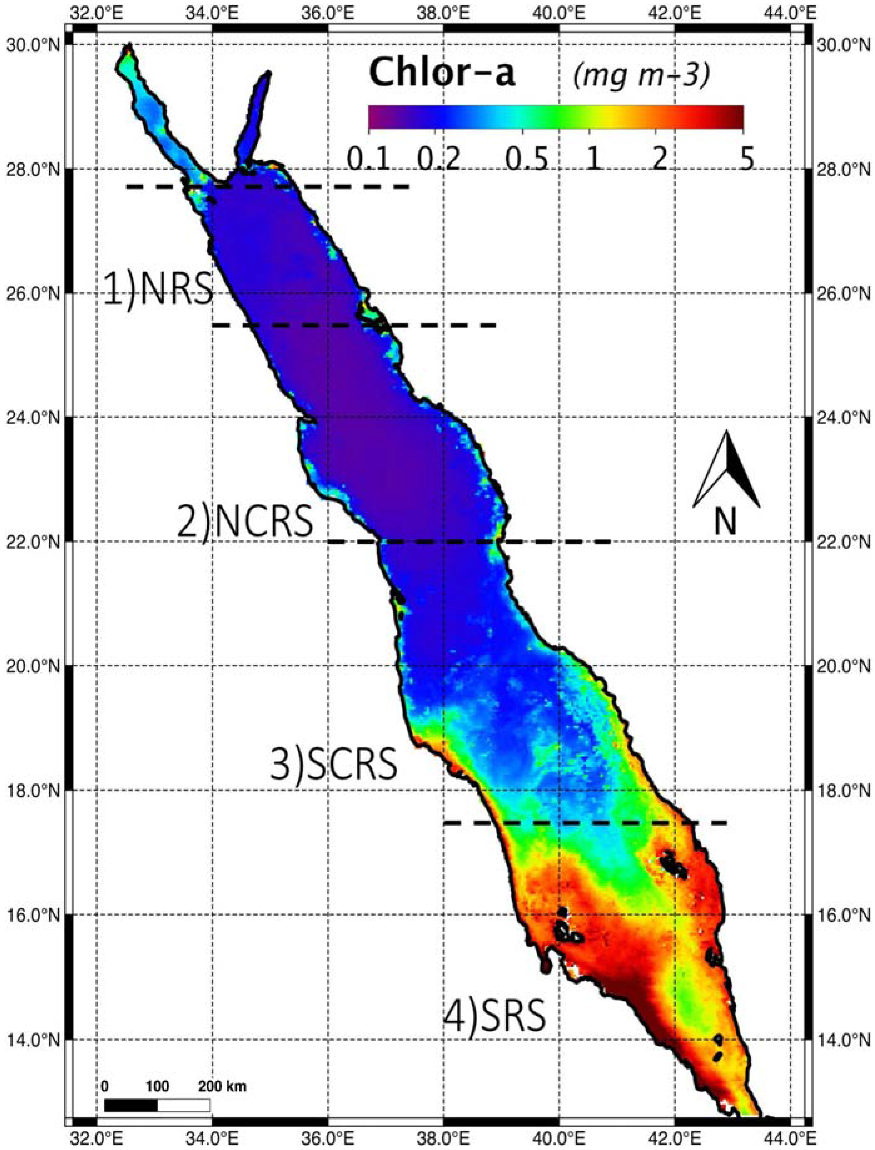
Figure 1. Moderate Resolution Imaging Spectroradiometer (MODIS) Aqua chlorophyll-a Chl-a (mg m−3) monthly averaged Level-3 composite for the Red Sea from July 2002 to May 2017. The four regions consecutively from north to south are the NRS, NCRS, SCRS and SRS. (This figure can be compared to Figure 2a from [17].)
Remotesensing 09 00778 g001
Figure 2. Hovmöller latitude-time plot for the four regions of Red Sea from January 2012 to December 2015. (Left) Chl-a (mg/m3) merged Level-3 Ocean Color Climate Change Initiative (OC-CCI) 4 km monthly data, (Right) MODIS-Aqua Chl-a (mg m−3) Level-3 4 km monthly data. The individual rows correspond to: (a) Northern Red Sea (NRS) (b) North Central Red Sea (NCRS) (c) South Central Red Sea (SCRS) (d) Southern Red Sea (SRS). Note the difference in the scales between the left and right sets of panels.
Remotesensing 09 00778 g002
Figure 3. Time series analysis of chlorophyll-a concentration in the Red Sea. (a) Area average of MODIS Aqua Chl-a concentration (mg m−3) monthly data from January 2012 to December 2016 over four regions of Red Sea (b) South Central Red Sea daily OC-CCI Chl-a concentration (mg m−3) from 1 June to 7 July for each year from 2012 to 2016.
Remotesensing 09 00778 g003
Figure 4. Chl-a concentrations in the Red Sea for different time periods (a) The OC-CCI Chl-a (mg m−3) merged level-3 5-day composite, from 25 June 2015 to 29 June 2015, (b) the OC-CCI Chl-a merged level-3 monthly composite for June 2015, (c) the MODIS Terra Chl-a level-3 monthly composite of June 2015, (d) the MODIS Terra Chl-a level-3 monthly climatology composite for June for all years from 2000 to 2015 and (e) MODIS Terra Chl-a level-3 4-km annual composite for 2015.
Remotesensing 09 00778 g004
Figure 5. Daily variability from 21 June until 30 June 2015 for (a) Chl-a, (b) mixed layer depth (MLD), (c) sea surface height (SSH), (d) sea surface temperature (SST).
Remotesensing 09 00778 g005
Figure 6. Ocean Surface Current Analysis Real-time (OSCAR) third-degree resolution ocean surface currents (m s−1) for (a) 17 to 21 June, (b) 22 to 26 June, (c) 27 June to 1 July 2015.
Remotesensing 09 00778 g006
Figure 7. The Tokar Wind Jet represented by (Left) MODIS-Terra true-color composite image of a dust event induced by the Jet on 23 June 2015 and (Right) Advanced Scatterometer (ASCAT) Level 3 wind field stress (pascal) on 24 June 2015.
Remotesensing 09 00778 g007
Figure 8. Time series of scaled anomalies for the SCRS for Chl-a and SST from MODIS-Aqua and dust aerosol optical depth (DAOD) from MERRA-2. The red box indicates the period from April to June 2015 including the largest anomalies in both DAOD and Chl-a.
Remotesensing 09 00778 g008
Figure 9. Monthly lag correlation between dust aerosol optical depth (DAOD) and Chl-a (solid) and SST and Chl-a (dot-dashed). Dashed lines show the limits of three standard deviations for a white noise process. The red box shows that the 2-month lag correlations exceed this level for both relationships.
Remotesensing 09 00778 g009
Figure 10. Sketch of the two circulation patterns in the Strait of Bab El Mandeb in the southern Red Sea. (Top) winter circulation. (Bottom) summer circulation. SW: surface water; GAIW: Gulf of Aden intermediate water; RSOW: Red Sea outflow water. (This figure is taken from [2] and used with permission).
Remotesensing 09 00778 g010
Table 1. Four Regions of the Red Sea; NRS: Northern Red Sea; NCRS: North Central Red Sea; SCRS: South Central Red Sea; SRS: Southern Red Sea.
Region NumberRegion NameNorth EndSouth End
1NRS27.7°N25.5°N
2NCRS25.5°N22°N
3SCRS22°N17.5°N
4SRS17.5°N12.8°N
Table 2. The characteristics and source of data used in this study. OC-CCI: Ocean Color Climate Change Initiative; GHRSST: Group for High Resolution Sea Surface Temperature; ASCAT: Advanced Scatterometer; OSCAR: Ocean Surface Current Analyses Real-time; MLD: mixed layer depth; SSH: sea surface height; AOD: aerosol optical depth; HYCOM: HYbrid Coordinate Ocean Model; SST: sea surface temperature.
Data NameProductLevelSpatial ResolutionTemporal ResolutionWeb Link
MODIS Chl-a (Terra & Aqua)MOD21/MYD2134 kmMonthlyhttps://oceancolor.gsfc.nasa.gov/cgi/l3
OC-CCI V3 dataOC-CCI Chl-a34 kmDaily/Monthlyhttps://www.oceancolour.org/portal
SSTGHRSST40.05°Dailyhttp://apdrc.soest.hawaii.edu /las/v6/constrain?var=11674
WindASCAT20.25°Dailyhttp://apdrc.soest.hawaii.edu /las/v6/dataset?catitem=11683
Ocean Surface CurrentOSCAR41/3°5-dayhttp://apdrc.soest.hawaii.edu/las/v6/constrain?var=2136
HYCOM ModelMLD-1/12°Dailyhttp://apdrc.soest.hawaii.edu/las/v6/constrain?var=10471
SSH-1/12°Dailyhttp://apdrc.soest.hawaii.edu/las/v6/constrain?var=10472
MODIS AOD (Terra & Aqua)MOD04/MYD0423 kmDailyhttps://worldview.earthdata.nasa.gov/

