
A Novel Spaceborne Sliding Spotlight Range Sweep Synthetic Aperture Radar: System and Imaging


1
Department of Electronic Engineering, Tsinghua University, Beijing 100084, China
2
School of Electronic Information Engineering, Beihang University, Beijing 100191, China
*
Author to whom correspondence should be addressed.
Remote Sens. 2017, 9(8), 783; https://doi.org/10.3390/rs9080783
Submission received: 10 May 2017
/
Revised: 18 July 2017
/
Accepted: 26 July 2017
/
Published: 31 July 2017
Abstract
:In this paper, a new Spaceborne Sliding Spotlight Range Sweep Synthetic Aperture Radar (SSS-RSSAR) is proposed to generate a high-resolution image of a Region of Interest (ROI) tilted with respect to the satellite track. Comparing to the traditional Spaceborne Sliding Spotlight Synthetic Aperture Radar (SSS-SAR), the SSS-RSSAR is superior in contributing to less data amount, lighter computational load and hence higher observation efficiency. Unlike the Spaceborne Stripmap Range Sweep Synthetic Aperture Radar (SS-RSSAR) proposed in a previous paper, the SSS-RSSAR not only continuously sweeps the beam in range for the ROI tracking, but also in azimuth to enlarge the synthetic aperture for an improved azimuth resolution. Two aspects of the SSS-RSSAR are focused: system and imaging. For the system part, a Continuous Varying Pulse Interval (CVPI) technique is proposed to avoid the transmission blockage problem by non-uniformly adjusting the pulse intervals based on the geometry. For the imaging part, a Modified Polar Format Algorithm (MPFA) is proposed to accommodate the original polar format algorithm to the echo received with the CVPI technique. Moreover, an integrate system parameter design flow for the SSS-RSSAR is also suggested. The presented approach is evaluated by exploiting the point target simulations.
1. Introduction
The Spaceborne Synthetic Aperture Radar (SAR) has dozens of operation modes, such as the stripmap mode, ScanSAR mode, TOPS mode, spotlight mode and the sliding spotlight mode, to image regions of interest (ROI) with variant combination of resolutions and swaths [1,2,3,4,5,6,7,8]. Despite the differences of these modes, they have one thing in common: their Beam Illumination Strip (BIS) (except for the spotlight mode) are all along the satellite ground-track direction [9,10,11,12,13]. As a result, for most current SAR satellites that move in near-polar orbits, their BISs are all nearly along north–south directions, whatever modes they operate in. In this case, if a ROI is tilted with respect to the satellite orbit and has a span wider than the cross-track swath of the BIS as shown in Figure 1a, more strips should be used to fully cover the tilted ROI. The seismic fault is a typical kind of such tilted ROI. To implement full coverage, one strategy is to use the ScanSAR mode or TOPS mode by dividing the whole Data Acquisition Period (DAP) into multiple bursts for multiple sub-strips by sacrificing the azimuth resolution. Another strategy is to use multiple orbits of observation by sacrificing the DAP. Though a recent Staggered SAR mode can image a much wider swath without the resolution scarification or DAP prolongation [14,15,16], it is, along with the former two strategies, to induce large amount of invalid data from disinterested regions such as those marked as Region E in Figure 1a. In sum, all these methods have inevitable drawbacks and thus are not the best solutions for the problem of imaging a tilted-with-orbit ROI in high resolutions and with a high data utilization efficiency.
To solve this problem, a Spaceborne Stripmap Range Sweep SAR (SS-RSSAR) has been proposed in a previous paper to generate a ROI-matched BIS by continuously sweeping the beam in elevation [17]. However, restricted by its fixed azimuth antenna pointing, the SS-RSSAR can only image a ROI in a stripmap-level azimuth resolution. In this paper a new Spaceborne Sliding Spotlight Range Sweep SAR (SSS-RSSAR) is proposed to achieve a higher azimuth resolution than the SS-RSSAR by not only continuously sweeping the beam in range for the ROI tracking, but also in azimuth to achieve an enlarged synthetic aperture for an improved azimuth resolution as shown in Figure 1b. Two major aspects of the SSS-RSSAR are to be focused in this paper: the system design and the imaging technique. The former part determines how the echo from the ROI should be collected and the latter part discusses how this echo should be focused. They serve as the basis for the new SSS-RSSAR theory.
Similar to the SS-RSSAR mode, the SSS-RSSAR’s Central Beam Pointing (CBP), which denotes the beam pointing at the central data acquisition time, is arranged to be perpendicular to the BIS for a good balance between the imaging swath and the signal-to-noise ratio [17]. In this case, the SSS-RSSAR is likely to operate with a large squint angle if the ROI is highly squinted with respect to the satellite orbit. As the radar antenna cannot receive while transmitting [18], the SSS-RSSAR is likely to suffer from the problem of transmission blockage due to the serious slant range variation caused by the continuous Two Dimensional (2D) beam steering. Aiming at overcoming this problem, a new Continuous Varying Pulse Interval (CVPI) technique is employed by the SSS-RSSAR to counteract the slant range variation by continuously adjusting the Pulse Intervals (PIs) based on the instant Central Beam Slant Range (CBSR), defined as the slant range from the SAR antenna center to the ground beam pointing. The core strategy of the CVPI technique is to locate the echo from the ROI at the central part of every PI. In this case, the space that can be used for the non-blocked echo receiving can be maximized. Due to the spatial variation of the CBSR, the SSS-RSSAR is characterized by non-uniform azimuth sampling, where the azimuth dependent PI array can be conveniently described by a fifth-order polynomial.
Due to the perpendicular-to-BIS CBP and its resulted large squint geometry, the echo is to suffer from serious 2D coupling and therefore, the imaging algorithm applied for the SSS-RSSAR should be carefully chosen. The basic Back Projection Algorithm (BPA) is not preferred due to its cost-inefficient O (N3) computational load [19]. The frequency domain algorithms that can be used for large-squint imaging, such as the Range Doppler Algorithm (RDA), Chirp Scaling Algorithm (CSA) and Range Migration Algorithm (RMA) [20,21,22], are all not ideal choices. This is because, if processed by these algorithms, the slant range that has been counteracted by the CVPI technique should be added back to the echo by using the zero padding, resulting in a much larger total data amount. The Polar Format Algorithm (PFA) seems to be the only frequency domain based algorithm that is capable of implementing a fast processing speed and a high data utilization efficiency [3,23]. However, due to the non-uniform azimuth sampling caused by the CVPI technique, the PFA cannot be directly applied for the SSS-RSSAR imaging. In this paper, a Modified PFA (MPFA) is proposed to focus the SSS-RSSAR’s echo received with the CVPI technique. The main modifications include an updated 2D dechirp filter and an interpolation-based data format correction based on a new wavenumber expression with respect to the CVPI technique.
Based on the CVPI technique and the MPFA imaging method, this study will further discuss the parameter design methods for the SSS-RSSAR. Firstly, based on the analyses for the least required range sample number, an optimized pulse width can be achieved. Then, based on the discussion on the least required azimuth sample, the referential pulse interval used for initiating the non-uniform PI array generation can be calculated. Generally speaking, the carrier frequency and the chirp rate are both constant during the whole DAP. For the SSS-RSSAR, however, the constant carrier frequency and chirp rate will lead to serious spatial variation of the wavenumber and therefore, the range wavenumber bandwidth after the MPFA processing will be seriously compressed, leading to a much decreased range resolution. To overcome this shortage, a new Parameter-Adjusting (PA) technique is proposed to mitigate the range wavenumber variation by adjusting the carrier frequency and the chirp rate pulse by pulse based on the instant data acquisition geometry. The methods of designing the sliding spotlight factor and the DAP are also introduced. Finally, an integrate parameter design flow for the SSS-RSSAR is provided.
The advantages of the SSS-RSSAR over the traditional Spaceborne Sliding Spotlight SAR (SSS-SAR) are also analyzed, mainly from two aspects: the total data amount and the total computational load. These analyses are made based on the assumption that both the SSS-RSSAR and the traditional SSS-SAR have perpendicular-to-BIS CBP. Based on the total data amount, the computational loads of the algorithms, including the MPFA, RDA, CSA and RMA, are compared. While the computational load of the MPFA is derived based on the total data amount collected from the tilted along-ROI BIS, the derivation of the computational loads of the RDA, CSA and RMA, on the other hand, are made based on the total data amount with respect to the parallel-to-orbit BIS. The reasons of choosing different data sets for the computational load comparison are: firstly, except for the MPFA, the echo of the SSS-RSSAR with the parameters specially designed based on the MPFA cannot be focused by the other algorithms. Secondly, if the algorithms such as the RDA, CSA and RMA were used for focusing, the parallel-to-orbit BIS would be the best data acquisition mode with the least data amount and lightest signal coupling. As has been demonstrated by the simulation experiments, comparing to the traditional SSS-SAR, the SSS-RSSAR contributes to a better performance as it requires less total data amount and lighter computational load in imaging a moderate-swath tilted-with-orbit ROI in a high resolution level.
The paper is arranged as follows. Section 2 discusses the CVPI technique for the non-uniform azimuth sampling. Section 3 discusses the MPFA for the SSS-RSSAR imaging. Section 4 discusses the parameter design methods for the SSS-RSSAR. Section 5 compares the total data mount and the total computational load between the SSS-RSSAR and the traditional SSS-SAR. The presented approach is evaluated in Section 6 by using the point target simulations. The study is summarized in Section 7 with a brief plan for the next-step research.
2. Continuous Varying Pulse Interval Technique
Similar to the discussion for the SS-RSSAR in [17], the CBP of the SSS-RSSAR is assumed to point vertically to the ROI strip as shown in Figure 2, where m denotes the azimuth sampling index and m = 0 denotes the central data acquisition time. The antenna should be continuously manipulated in two dimensions to make sure the ground beam center always moves along the X-axis. A Cartesian coordinate is built to simplify the discussions. The origin O overlaps with the swath center. The X-axis is along the along-BIS direction. The Y-axis is along the cross-BIS direction in the ground plane, corresponding to the projection of CBSR at m = 0. The Z-axis is vertical to the ground plane and points inversely to the Earth center. The directions along the X- and Y-axis are defined as the azimuth and range directions, respectively.
Other parameters are defined as follows. H denotes the constant height of the SSS-RSSAR. θ denotes the tile angle between the X-axis and the nadir of the satellite tract. β denotes the instant look angle with respect to the swath center O. α denotes the instant azimuth angle between the Y-axis and the projection of the instant slant range from the SAR antenna center to the swath center O. βc and Rc0 denote the central look angle and the central slant range with respect to the swath center at m = 0. p and k denote two azimuth sampling indexes before and after the central data acquisition time. The CBSR at m = p and m = k are Rcp and Rck, respectively. Wr and Wa denote the expected range and azimuth BIS swaths. The real curved satellite orbit is assumed to be rectilinear here for simplicity.
Vs and Vg denote the satellite velocity and the beam velocity along the X-axis, respectively. They have the following relationship
where η denotes the sliding spotlight factor. The SS-RSSAR mode discussed in [17] corresponds to the very case with η = 1. If a traditional constant PI was applied for the SSS-RSSAR, the continuous range-azimuth beam sweeping would lead to slant range variation and inevitably cause the transmission blockage. To solve this problem, a new CVPI technique is developed for the full echo receiving by non-uniformly adjusting the PIs based on the instant data acquisition geometry. Unlike the Multi-Interval Sampling (MIS) technique used by the SS-RSSAR [17], the CVPI technique continuously varies the PI sequence by employing a polynomial fitting method. Furthermore, unlike the MIS technique that changes the number of PI between the transmitting and receiving, the CVPI technique keeps this number unchanged during the entire DAP. Thus, the CVPI-based non-uniform azimuth sampling array will be easier to design and generate.
The key idea of the CVPI method is to locate the echo of the targets along X-axis to the center of every PI. In this case, all the echoes from the ROI can be set around the central part of every PI. In other words, the expected PI variation should counteract the CBSR variation within the DAP. For the three sampling positions with the CBSRs Rcp, Rc0 and Rck in Figure 2, the expected CVPI-based echo distribution is shown in Figure 3, where, despite the differences of the Rcp, Rc0 and Rck, all the echoes are all located at the central part of their individual PIs.
A fifth-order polynomial of the azimuth time is used for the PI variation description. In this case, the mth PI can be expressed by
where μn denotes the polynomial coefficient and t denotes the azimuth time. A referential PI, denoted as PI0, should be set firstly to initiate the non-uniform PI array generation. Notice that PI0 should be both large enough to enclose all the echoes from the ROI strip and small enough to avoid the Doppler aliasing. The detailed method of calculating PI0 will be discussed in Section 4. Based on a given PI0, the PI number M between the transmitting and receiving should then be calculated as
where c denotes the speed of light and the operator (·) computes the maximum integer not larger than the input number. Then by using the stop-go model, the CBSR at the mth sample yields
By substituting Equation (2) into Equation (4), the latter can be rewritten in the matrix formation as
where
where Na denotes the azimuth sample number. The elements of Matrix A and B, denoted by amj and bm, yield
The vector μ can be solved out based on the least-square method. Note that the pulse intervals are no longer uniform, the azimuth sampling time t should be calculated iteratively as
where t0 denotes the start time of the data acquisition, followed by a PI equaling to PI0.
3. Modified Polar Format Algorithm
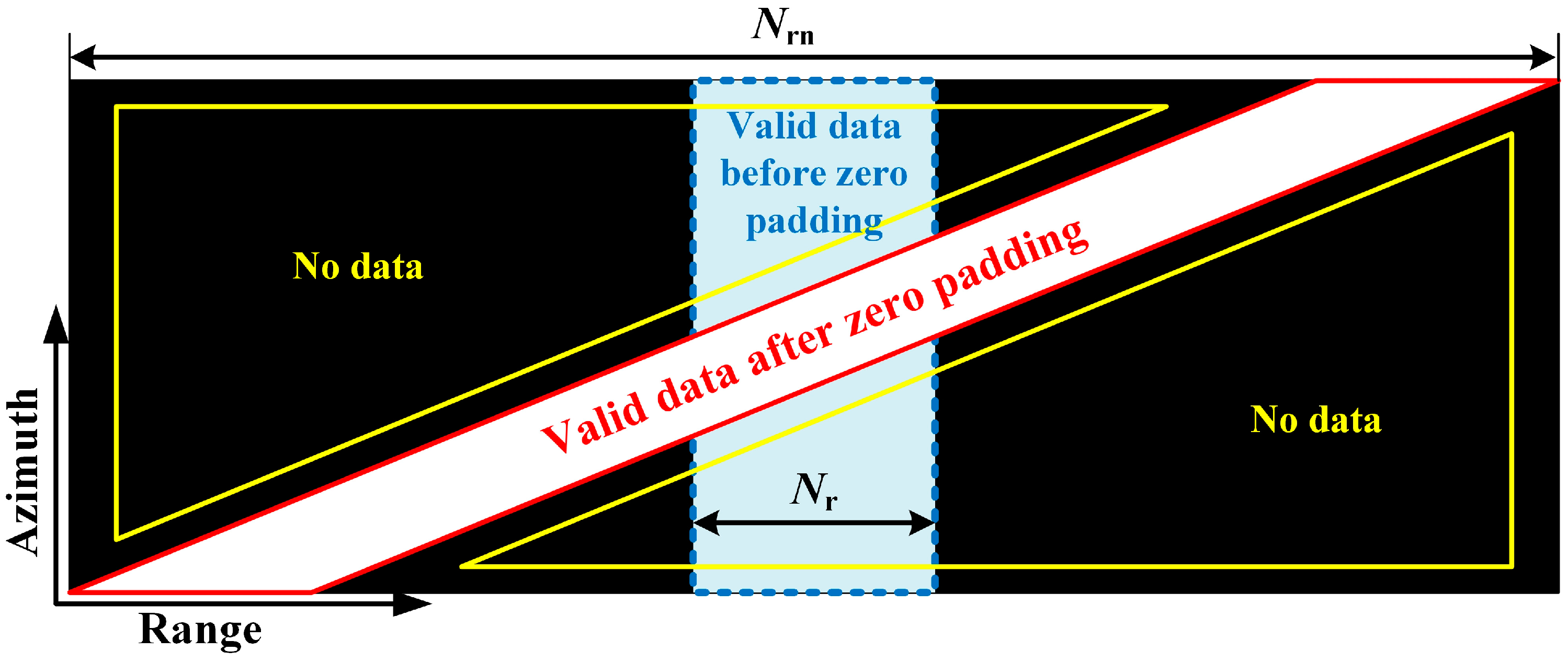
The continuous azimuth-range beam steering of the SSS-RSSAR will induce serious 2D signal coupling to the echo, which, as a result, will be hard to focus. If processed by the algorithms such as the RDA, CSA and RMA, the slant range variation that has been removed by the CVPI method should be added back by zero-padding the echo in range as shown in Figure 4, where Nr and Nrn denote the range sample number before and after the zero padding, respectively. The blue square denotes the valid data received with the CVPI technique and the white region denotes the valid data to which the slant range variation has been added back. It is clear that the processing efficiency would be dramatically decreased due to the increased invalid data marked by the yellow triangles.
The PFA is the only frequency-domain algorithm that can focus the echo with no necessity of recovering the full range migration and thus, will not induce additional invalid data. However, due to the employed CVPI technique, the azimuth sampling of the SSS-RSSAR is no longer uniform and thus, the traditional PFA cannot be directly applied for the SSS-RSSAR imaging. In this section, a MPFA is proposed with a new 2D dechirp filter and an interpolation-based data correction manipulation based on a new wavenumber depending on the CVPI technique.
3.1. Modified Two Dimensional Dechirp
While the SSS-RSSAR does not apply the dechirp-on-receive mechanism, the chirp characteristic of the echo should be removed firstly, along both the range and azimuth dimensions. In the case of a transmitted LFM signal, the backscattered echo of an arbitrary Target S can be digitally expressed as
where m and i denote the azimuth and range sample indexes, respectively; fc denotes the carrier frequency; γ denotes the chirp rate of the LFM signal; Tp denotes the pulse width; Fs denotes the sampling rate; and Rs denotes the instant slant range for Target S. Na and Nr denote the azimuth and the range sample numbers, respectively. Nas denotes a smaller-than-Na azimuth sample number for Target S. ms denote azimuth position where the beam center illuminates Target S. τd denotes the time delay. While τd is a constant for the traditional constant-PI SAR, for the SSS-RSSAR, τd is azimuth-sensitive due to the CVPI technique as
Based on the echo in Equation (9), the new 2D dechirp filter of the MPFA yields
where Rref denotes the instant slant range from the antenna to the swath center. By multiplying the echo in Equation (9) with Fdechirp, the dechirped signal yields
where ΔRs denotes differential slant range as
3.2. Residual Video Phase Removal
The second phase term in Equation (12) denotes the Residual Video Phase (RVP) that impacts SAR imagery because the displacement between the two waveforms varies with time as the two-way range to a scatterer changes over a coherent processing interval [3]. In the time domain the RVP is hard to compensate because ΔRs is space-variant. However, the RVP can be conveniently compensated in the frequency domain.
By making a range Fast Fourier Transform (FFT) along the i dimension, the range spectrum of the signal in Equation (12) yields
Based on the sinc(·) function in Equation (14), the target is found to be focused at i’s as
By substituting Equation (15) into Equation (14), the latter equation can be rewritten as
Aiming at compensating the second quadratic phases in Equation (16) at i’ = i’s, the RVP removal filter can be generated as
By multiplying FRVP with range spectrum of Es1 and converting the signal back to the range time domain via the range Inverse FFT (IFFT), the signal yields
3.3. Interpolation-Based Data Format Correction
As the 2D dechirp has uniquely mapped the signal from the time domain to the frequency domain, the range-azimuth signal coupling can be removed by the interpolation. Firstly, a new line-of-sight wavenumber KR is defined as
Different from the conventional wavenumber, the new wavenumber in Equation (19) contains the time delay induced by the CVPI technique. By substituting Equation (19) into Equation (18) and neglecting the amplitude terms, Equation (18) can be rewritten as
The projections of KR along the X- and Y-axis, denoted as KX and KY, respectively, yield
By assuming that the transmitted signal has a planar waveform, the differential slant range ΔRs can be approximated as [3,23].
where xs and ys are the X and Y coordinates of Target S. By substituting Equation (22) into Equation (20), Es2 can be approximated as
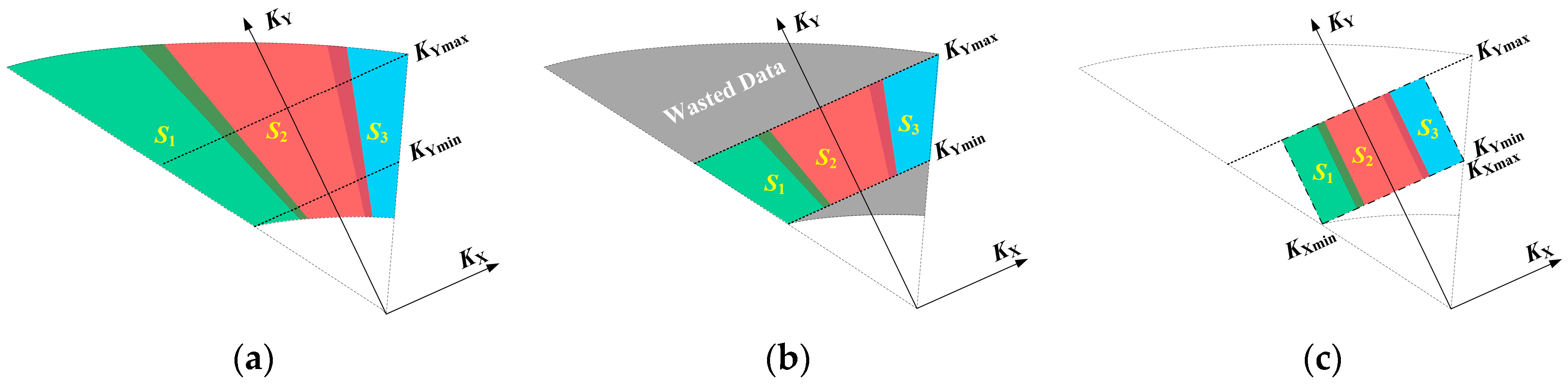
By assuming three targets, denoted as Target S1, S2 and S3, are located along the X-axis in sequence, their echoes after the RVP removal processing will be distributed in a polar format in the wavenumber as shown in Figure 5a. Then a range interpolation is applied to eliminate the spatial variation of the range wavenumber as
where K’Y denotes the referential range wavenumber as
where KYmin and KYmax denote the minimum and maximum values of K’Y, respectively, as
After the range interpolation, the signal is converted from the polar format to the keystone format as shown in Figure 5b, as
Then an azimuth interpolation is employed to convert the data from the Keystone format to the rectangular format as
where the azimuth referential wavenumber K’X yields
where KXmin and KXmax denote the minimum and maximum values of K’X, respectively, as
The resulted rectangular-format signal is shown in Figure 5c and can be expressed as
By conducting the FFT along both the range and azimuth dimensions, the final focused image can be achieved.
4. System Parameter Design
4.1. Range Sample Number and Pulse Width
For a traditional SAR system, the sampling rate should be higher than the bandwidth of the transmitted LFM signal to avoid aliasing. For the SSS-RSSAR, however, as the range LFM characteristic is removed by the 2D dechirp processing, the range non-aliasing sampling restriction is different from the traditional SAR systems.
For an observation task with an expected ground range resolution ρr, the bandwidth of the LFM signal, denoted by Br, can be set as
However, after the 2D dechirp, there will be a unique mapping between the target position and its frequency [3] and thus, the signal will have a new bandwidth Brn based on the geometry in Figure 2 as
The non-aliasing sampling rate Fs should be slightly higher than the new bandwidth Brn as
where σ denotes an oversampling factor ranging from 1.1~1.3. The chirp rate γ in Equation (33) can be rewritten based on the characteristic of the LFM signal as
By substituting Equations (32), (33) and (35) into Equation (34), the sampling rate can be rewritten as
On the other aspect, the echo length τw can be estimated by
The least required range sample number Nrmin can be achieved by multiplying Fs with τw as
On the other hand, Nr also has an upper limit Nrmax corresponding to the case that all the space of the minimum PI is used for the data receiving as
The final range sample number Nr can then be set slightly higher than Nrmin but lower than Nrmax. Based on Equation (38), it is clear that the longer the Tp, the smaller the required range sample number. Thus, the pulse width should be elongated as much as possible to decrease the least required total data amount. However, Tp cannot be elongated limitlessly. The upper limit for Tp, denoted as Tpmax, corresponds to the case that the echo length τw equals to the minimum PI as
For a real SSS-RSSAR system, Tp should be slightly smaller than the theoretical upper limit Tpmax to leave enough space for the antenna to switch between the transmitting and receiving.
4.2. Azimuth Sample Number and Referential Pulse Interval
As has been discussion in Section 2, the whole non-uniform PI array should be generated based on an initially set referential PI, the design of which, as will be seen below, is based on the least required non-aliasing azimuth sample number. Similar to the range bandwidth, the azimuth bandwidth of the SSS-RSSAR will also be changed by the 2D dechirp. After the range interpolation, the azimuth bandwidth of the total wavenumber spectrum, denoted as ΔKX, yields
Note that ΔKX is actually wider than the azimuth wavenumber bandwidth of the signal because the total azimuth sample number Na is larger than the azimuth sample number for an individual target, such as Nas in Equation (9). To avoid the azimuth aliasing, the azimuth swath of the reconstructed image should be wider than the BIS swath along the X-axis as
By substituting Equations (25), (41) into Equation (42), the least required azimuth sample number Namin can be estimated by assuming i = 0 for simplicity as
The final azimuth sample number Na can be set slightly larger than Namin. Then by assuming the length of orbit over which the SSS-RSSAR flies during the DAP is D, the referential pulse interval PI0 can be achieved as
Based on Equation (44) and the CVPI technique, the total non-uniform azimuth sampling array can be generated iteratively based on Equation (8). Due to the PI variation, the validity of the PI array should be checked to ensure that the echo from the ROI can be fully recorded in every PI as
Otherwise, PI0 should be further elongated for a new PI array generation until the condition in Equation (45) can be satisfied.
4.3. Carrier Frequency and Chirp Rate
By comparing Figure 5a,b, it is clear that due to the serious spatial variation of the range wavenumber, a large ratio of data, marked by the grey regions, have been wasted, resulting in a much compressed range bandwidth of KY and a degraded range resolution. In an extreme case where KYmax is smaller than KYmin, it is even impossible to implement focusing.
Based on Equation (21), the spatial variation of KY is caused by the variations of the instant look angle β and azimuth angle α and the azimuth-dependent time delay τd. These two kinds of variations have different impacts on KY. As the angle-related range wavenumber variation is range-independent, it can be fully counteracted by using the PA method discussed in [23]. On the other aspect, the range wavenumber variation caused by τd relies on both the range and azimuth, hence cannot be fully compensated by the PA method. As a result, the echo cannot be directly received with the Keystone format distribution, as shown in Figure 5b, by adjusting the parameters pulse by pulse. However, we can develop a new PA technique based on the expression of the range wavenumber to suppress the spatial variation of KY and to minimize the loss of the range wavenumber bandwidth while conducting the range interpolation.
Similar to the PA technique in [23], the new PA technique adjusts the carrier frequency fc and the chirp rate γ pulse by pulse based on the instant data acquisition geometry as
where fc0 and γ0 denote the constant referential carrier frequency and the constant referential chirp rate, respectively. The first faction is to counteract the angle-related spatial variation and the second faction is to suppress the spatial variation caused by τd.
By applying the new PA technique in Equation (46), the recorded polar format data are shown in Figure 6a, where the spatial variation of the range wavenumber has been greatly suppressed. In this case, the Keystone format data generated by the range interpolation, as shown in Figure 6b, suffer from a much less range wavenumber bandwidth loss. The rectangular format data after the azimuth interpolation are shown in Figure 6c. Comparing Figure 5 and Figure 6, it is clear that the ratio of the wasted data has been effectively decreased benefiting from the new PA manipulation in Equation (46).
4.4. Sliding Spotlight Factor and Data Acquisition Period
The sliding spotlight factor η of the SSS-RSSAR determines how fast the beam is steered in azimuth. Similar to the traditional sliding spotlight SAR system, the sliding spotlight factor of the SSS-RSSAR can be estimated by the time of the azimuth resolution improvement with respect to its stripmap mode, the SS-RSSAR, as
where ρa and ρa0 denote the azimuth resolutions of the SSS-RSSAR and the SS-RSSAR images, respectively. Based on the data acquisition geometry of the SS-RSSAR in [17], ρa0 can be estimated by
where ψ and Ba0 denotes the central squint angle and Doppler bandwidth with respect to the swath center, respectively. By assuming the beam width is ϕa, Ba0 can be estimated by
By substituting Equation (49) into Equation (48), ρa0 can be rewritten as
By substituting Equation (50) into Equation (47) and replacing the carrier frequency fc with fc0 if the new PA technique is adopted, the sliding spotlight factor η of the SSS-RSSAR can be set as
To ensure that all targets within the ROI can be fully illuminated, the minimum DAP ta can be estimated as
By substituting Equations (1) and (51) into Equation (52), ta can be rewritten as
4.5. Integrate Parameter Design Flow
Based on the above discussions, the steps of system parameter design for the SSS-RSSAR can be summarized as:
Step 1. Set the parameters of an observation task, including the 2D swaths (Wa and Wr) and 2D resolutions (ρa and ρr); Set the referential carrier frequency fc0.
Step 2. Choose a proper orbit for the data acquisition with the parameters including the orbit height H, platform velocity Vs and tilt angle θ; Find the SAR position at the central data acquisition time based on the perpendicular-to-BIS CBP; Compute the central look angle βc and the central slant range Rc0.
Step 3. Compute the sliding spotlight factor η based on Equation (51). Compute the DAP ta based on Equation (53). Compute the starting and ending SSS-RSSAR positions, denoted as Ps and Pe, within the DAP. Compute the along-orbit distance D between Ps and Pe. Compute the azimuth angles αs and αe for Ps and Pe, respectively.
Step 4. Compute the azimuth bandwidth of the wavenumber spectrum ΔKX based on Equation (41) by replacing α(−Na/2) and α(Na/2) with αs and αe, respectively. Compute the minimum azimuth sample number Namin based on (43). Set an azimuth sample number Na slightly higher than Namin. Compute the referential pulse interval PI0 based on Equation (44).
Step 5. Generate the non-uniform PI array by using the CVPI technique.
Step 6. Compute the maximum pulse width Tpmax based on Equation (40). Set a pulse interval Tp slightly lower than Tpmax. Compute the required referential chirp rate γ0 based on Equations (32) and (35). Compute the sampling rate Fs based on Equation (36). Compute the lower and upper limits for range sample number based on Equations (38) and (39), respectively. Set a range sample number Nr between these two limits.
Step 7. Compute the azimuth-dependent carrier frequency and chirp rate based on Equation (46).
The system parameter design flowchart for the SSS-RSSAR is shown in Figure 7.
5. Comparisons
In this section, the SSS-RSSAR and the traditional SSS-SAR are to be compared in two main aspects: the total sample number for the full data acquisition and the total computational loads for the raw data focusing.
5.1. Total Sample Number
As stated at the beginning of this paper, the advantage of the SSS-RSSAR over the traditional SSS-SAR is that the SSS-RSSAR can image a tilted ROI with a much narrower ROI-matched BIS and hence contribute to less total data amount. If the data acquisition were made using the traditional SSS-SAR, the BIS would be parallel to the satellite orbit. For this case, the most simple and effective geometry corresponds to a CBP with a zero squint angle for and being vertical to the parallel-to-orbit BIS. To fully cover the BIS of the SSS-RSSAR, the cross-BIS swath of the traditional SSS-SAR, denoted as WrT in Figure 2, yields
By replacing Wr in Equation (37) with WrT, the echo length of the traditional SSS-SAR τwT yields
Different from SSS-RSSAR, the sampling rate of the traditional SSS-SAR, denoted as FsT, should be calculated by substituting the bandwidth Br in Equation (32), instead of the dechirped one Brn in Equation (33), into Equation (34) as
The least required range sample number NrminT can be achieved by multiplying τwT and FsT as
On the other aspect, for an expected along-strip azimuth resolution ρa, the minimum Doppler bandwidth of a target, denoted as BaT, is
To avoid the azimuth aliasing, the maximum constant pulse interval, denoted as PIT, for the azimuth sampling should be
By employing the same beam width ϕa and the central beam slant range Rc0, the least required data acquisition period, denoted as taT, can be estimated by
where WaT denotes the along-track BIS swath of the traditional SSS-SAR as shown in Figure 2 as
The minimum azimuth sampling number, denoted as NaminT, can be computed by dividing taT in Equation (60) by PIT in Equation (59) as
By multiplying NrminT and NaminT, the total sample number for the traditional SSS-SAR, denotes as NtotalT, yields
Comparatively, the total sample number for the SSS-RSSAR, denoted as Ntotal, can be computed by multiplying Nrmin in Equation (38) and Namin in Equation (43) as
5.2. Total Computational Load
This section compares the total FLoat-point OPeration (FLOP) of the MPFA and other frequency domain imaging algorithms, including the RDA, CSA and RMA. The basic operations employed by these algorithms including the FFT/IFFT, complex multiply and interpolation. The computational loads of these basic operations are summarized in Table 1. Table 2 lists the computational load of the MPFA step by step.
There would be two major differences if the other algorithms such as the RDA, CSA and the RMA, instead of the MPFA, were used for imaging. Firstly, without the 2D dechirp to alter the range and azimuth bandwidths, the sampling rate should be set as FsT in Equation (56) and the referential pulse interval PI0 should be set as PIT in Equation (59), instead of the Fs in Equation (36) and the PI0 in Equation (44), respectively. Secondly, due to the brief discussions at the beginning of Section 3, all the RDA, CSA and RMA need to firstly recover the range migration that has been counteracted by the CVPI technique, resulting in a much larger new range sample number Nrn as shown in Figure 4. If the same squint CBP as shown in Figure 2 is used, the minimum value of Nrn, denoted as Nrnmin, can be estimated by
By comparing Equations (57) and (65), it is found that the only difference is the factor cos θ induced by the squint beam pointing. The minimum sample number can be regarded as the same as NaminT in Equation (62) as PIT is used to generate the PI array. In sum, the total sample number that needs to be processed is 1/cos θ time of the NtotalT in Equation (63). Thus far, it is clear that, if processed by the algorithms of RDA, CSA and RMA, a squint CBP will lead to no benefit but larger data mount and more serious signal coupling. Thus, the computational load analyses for the algorithms of RDA, CSA and RMA should be made based on the geometry with a broadside CBP as that of the traditional SSS-SAR. In this case, the least required total data amount can be minimized and the 2D signal coupling can be mitigated. In this case, the range, azimuth and total sample numbers for the algorithms of the RDA, CSA and RMA are the same with those in Equations (57), (62) and (63), resulting in the total computational loads in Table 3 [2].
6. Simulation and Discussion
The presented approach is to be evaluated via a simulated X-band SSS-RSSAR. Within a 5 km × 10 km (range × azimuth) ROI, 25 targets are uniformly distributed as shown in Figure 8. The expected resolutions are in 1.00 m × 1.31 m (range × azimuth). The key parameters used for the SSS-RSSAR simulation are listed in Table 4, where the basic parameters are those initially set for the SSS-RSSAR observation task and the derived parameters are those calculated based on the discussions in Section 4. No antenna weighting is used for the echo simulation.
Based on the simulation geometry and the basic parameters in Table 4, the DAP of the simulated SSS-RSSAR ranges from −2.49 s to 2.49 s with the CBSR variation as shown in Figure 9a. Based on the CBSR, the azimuth dependent PI array is generated as shown in Figure 9b. Figure 10a,b illustrate the echoes simulated by using and not using the CVPI technique. The while regions denote the valid data and the black regions denote no data. The constant PI used in generating Figure 10b is 190.5 μs, equaling to the 13,074th PI. While large amounts of data are lost when using the constant PI because of the transmission blockage in Figure 10b, the echo can be fully received with the CVPI technique as shown in Figure 10a. It is known that the longer the pulse width, the more serious the transmission blockage will be. Thus, the shortage of using a constant PI tends to be more serious for the SSS-RSSAR because it prefers a long pulse width. As a result, the CVPI technique has been demonstrated to be necessary and effective for the data acquisition of the SSS-RSSAR.
Based on the new PA technique, the azimuth-dependent carrier frequency and chirp rate are shown in Figure 11a,b, respectively. Figure 12 compares the range wavenumber KY when using and not using the new PA method. The red and blue lines denote the upper and lower limits of the range wavenumber spectrum and the green lines denote the upper and lower limits of range wavenumber of the valid data after the RVP removal. Figure 12a denotes the case where the new PA technique is used. The maximum and minimum values of KY almost overlap with KYmax and KYmin respectively, resulting in a range bandwidth of the wavenumber domain ΔKY around 8.8 rad/m. Note that as this bandwidth is actually wider than the real range wavenumber bandwidth of the valid data ΔKYs because the echoes of different targets have been aligned to the referential target (swath center) by the RVP removal manipulation. Based on Equations (19), (21) and (46), ΔKYs can be estimated as
By substituting the parameters in Table 4 into Equation (66), ΔKYs is calculated as 6.28 rad/s, which is not to be altered by the range interpolation. Comparatively, in Figure 11b where the carrier frequency and chirp rate always equal to their constant referential values fc0 and γ0, respectively, both the maximum and minimum values of KY are characterized with large spatial varieties and the range bandwidth of the wavenumber domain ΔKY is around 0.33 rad/m, much narrower than the range wavenumber bandwidth of the valid data ΔKYs. For this case, ΔKYs equals to ΔKY.
The difference of the range wavenumber bandwidth of the valid data will lead to different range resolution performances as shown in Figure 13, where the central swath target T33 is adopted for the resolution inspection. For the case where the new PA technique is used in Figure 13a, the range resolution of the focused image is 1.035 m. Comparatively, for the case where the traditional constant parameter strategy is used in Figure 13b, the range resolution is 18.846 m, degraded by around 18.8 times. By noticing that that the range wavenumber bandwidth of the valid data achieved with the new PA technique is 18.8 times high than that without the new PA technique, we can conclude that the improvement of the range resolution performance is caused by the expansion of the range wavenumber bandwidth contributed by the new PA technique. By comparing Figure 13a,b, we find the azimuth resolutions of the two cases are almost the same. This is because the azimuth samples corresponding to the beam dwell time of T33 are within the region restricted by A1 – A2 in Figure 12b. For the azimuth samples outside the A1 – A2 region, there would be no valid data after the range interpolation. Therefore, for the azimuth marginal targets such as T11, T31, T51, T15, T35, T55, etc., the azimuth resolutions would be degraded. Based on the results in Figure 11, Figure 12 and Figure 13, the benefits of applying the new PA technique for the SSS-RSSAR data acquisition have been demonstrated.
To assess the effectiveness of the MPFA for the SSS-RSSAR imaging, the contour plots of amplitudes of the focused marginal targets T11, T13, T15, T31, T33, T35, T51, T53 and T55 are inspected in Figure 14. The new PA technique is employed in generating the transmitted pulses. The indicators for the focusing quality evaluation, including the peak side lobe ratio (PSLR), integrate side lobe ratio (ISLR) and resolution, are listed in Table 5. The fact that for all the targets the PSLRs and ISLRs match well with their theoretical values, −10.26 dB and −9.8 dB, respectively, and that the measured resolutions match well with their expected performances in Table 4, the validity of the MPFA in focusing the SSS-RSSAR data has been demonstrated. The slight inconsistency of the azimuth resolutions in Table 5 is caused by the slight difference of the beam dwell time of different targets.
To demonstrate the advantages of the SSS-RSSAR over the traditional sliding spotlight SAR, the least required total sample numbers and the total computational load for imaging are shown in Figure 15 and Figure 16, respectively. The variation of the minimum total sample numbers of the SSS-RSSAR and the traditional SSS-SAR with respect to the range and azimuth swaths are shown in Figure 15a,b. The inspected range swath ranges from 1 km to 10 km and the inspected azimuth swath ranges from 1 to 20 km. It is found that while for a smaller ROI swath the total sample number of the SSS-RSSAR is much lower than that of the traditional SSS-SAR, for a large ROI swath, however, there would be no obvious advantage of the SSS-RSSAR because a large swath will lead to wider range and azimuth bandwidths after the 2D dechirp and thus, larger sampling rates, both in range and in azimuth, are required, accompanied with more sample numbers. This also implies that the SSS-RSSAR is especially suitable for imaging a moderate-swath ROI tilted with the satellite track in a high resolution. Note that, as the total sample number of the SSS-RSSAR 6477 × 23,492 (range × azimuth), as shown in Figure 15a, represents the least required number, the real total sample used for the simulation experiments is 7344 × 26,124 (range × azimuth), which turns to be higher than the least required value in observing the 5 km × 10 km (range × azimuth) tilted ROI.
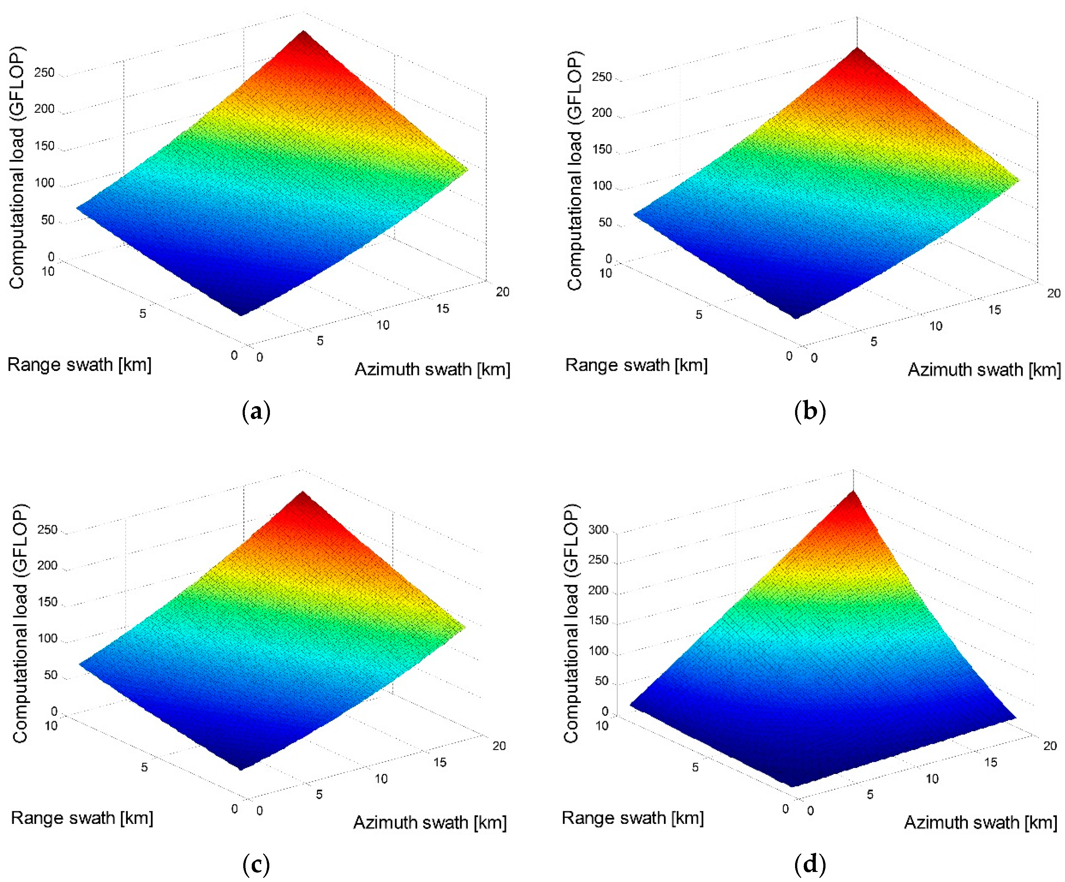
The least required total computational loads when using the MPFA and other imaging algorithms, including the RDA, CSA and RMA, are compared in Figure 16. Based on the discussion in Section 5.2, while the computational loads of the RDA, CSA and RMA are calculated based on the least total sample number in Figure 15b, the computational load of the MPFA is calculated based on the total sample number in Figure 15a. For the simulated case, the total computational loads of the RDA, CSA and RMA are 93.5 GFLOP, 86.6 GFLOP and 91.8 GFLOP, respectively. Comparatively, the total computational load of the MPFA is only 50.9 GFLOP, much lower than all those of the RDA, CSA and RMA. The comparisons in Figure 15 and Figure 16 have demonstrated that, for a moderate swath, the SSS-RSSAR is superior to the traditional SSS-SAR by contributing to less total data amount and lighter computational load for the imaging processing. This is the very motivation of proposing the SSS-RSSAR in this paper.
7. Conclusions
This study investigated the system design and imaging method for a new SSS-RSSAR that continuously steers its beam in azimuth and in range to generate a ROI-matched BIS. Comparing to the fixed azimuth pointing of the SS-RSSAR, the SSS-RSSAR is capable of implementing a wider synthetic aperture and achieving a higher azimuth resolution. The continuous range-azimuth beam steering of the SSS-RSSAR is to cause a wide range of slant range variation and hence lead to the problem of transmission blockage. Aiming at solving this problem, a new CVPI technique was used to mitigate the slant range variation by continuously adjusting the PI based on the instant data acquisition geometry. An MPFA was derived to focus the seriously coupled echo received in a highly squinted geometry due to the perpendicular-to-BIS CBP. Based on the CVPI technique and the MPFA method, an integrated system parameter design flow for the SSS-RSSAR has been suggested, including a new PA technique to suppress the spatial range wavenumber variation. The total data amount and the total computational load between the SSS-RSSAR and the traditional SSS-SAR have also been compared. Based on the simulation experiments, the advantages of the SSS-RSSAR in imaging a moderate-swath and tilted ROI in a high resolution over the traditional SSS-SAR have been demonstrated. Future research may include the development of an airborne prototype of the SSS-RSSAR for real-data based experiments.
Acknowledgments
This work was supported in part by the National Natural Science Foundation of China (No. 61601257 and No. 61371133), in part by the Major Project of China High-resolution Earth Observation (No. 30-Y20A12-9004-15/16), in part by the China Postdoctoral Science Foundation (No. 2016M591179) and in part by a special project with No. 30402010203.
Author Contributions
The work presented here was carried out in collaboration between all authors. Yan Wang, Jingwen Li, Jian Yang and Bing Sun defined the research theme. Yan Wang designed the methods and experiments, carried out the laboratory experiments, analyzed the data, interpreted the results and wrote the paper. All authors have contributed to, seen, and approved the manuscript.
Conflicts of Interest
The authors declare no conflict of interest.
References
- Curlander, J.C.; McDonough, R.N. Synthetic Aperture Radar: Systems and Signal Processing; Wiley: Hoboken, NJ, USA, 1991. [Google Scholar]
- Cumming, I.G.; Wong, F.H. Digital Processing of Synthetic Aperture Radar Data: Algorithms and Implementation; Artech House: Norwood, MA, USA, 2005. [Google Scholar]
- Carrara, W.G.; Goodman, R.S.; Majewski, R.M. Spotlight Synthetic Aperture Radar: Signal Processing Algorithms; Artech House: Boston, MA, USA, 1995. [Google Scholar]
- Moore, R.K.; Claassen, J.P.; Lin, Y.H. Scanning spaceborne synthetic aperture radar with integrated radiometer. IEEE Trans. Aerosp. Electron. Syst. 1981, 17, 410–420. [Google Scholar] [CrossRef]
- Zan, F.D.; Guarnieri, A.M. TOPSAR: Terrain observation by progressive scans. IEEE Trans. Geosci. Remote Sens. 2006, 44, 2352–2360. [Google Scholar] [CrossRef]
- Lanari, R.; Tesauro, M.; Sansosti, E.; Fornaro, G. Spotlight SAR data focusing based on a two-step processing approach. IEEE Trans. Geosci. Remote Sens. 2001, 39, 1993–2004. [Google Scholar] [CrossRef]
- Prats, P.; Scheiber, R.; Mittermayer, J.; Meta, A.; Moreira, A. Processing of Sliding Spotlight and TOPS SAR Data Using Baseband Azimuth Scaling. IEEE Trans. Geosci. Remote Sens. 2010, 48, 770–780. [Google Scholar] [CrossRef] [Green Version]
- Mittermayer, J.; Lord, R.; Boerner, E. Sliding spotlight SAR processing for TerraSAR-X using a new formulation of the extended chirp scaling algorithm. In Proceedings of the 2003 IEEE International Geoscience and Remote Sensing Symposium (IGARSS ’03), Toulouse, France, 21–25 July 2003; Volume 3, pp. 1462–1464. [Google Scholar]
- Arikawa, Y.; Saruwatari, H.; Hatooka, Y.; Suzuki, S. ALOS-2 launch and early orbit operation result. In Proceedings of the 2014 IEEE International Geoscience and Remote Sensing Symposium (IGARSS), Quebec, QC, Canada, 13–18 July 2014; pp. 3406–3409. [Google Scholar]
- Werninghaus, R.; Buckreuss, S. The TerraSAR-X Mission and System Design. IEEE Trans. Geosci. Remote Sens. 2010, 48, 606–614. [Google Scholar] [CrossRef] [Green Version]
- Torres, R.; Snoeij, P.; Geudtner, D.; Bibby, D.; Davidson, M.; Attema, E.; Potin, P.; Rommen, B.; Floury, N.; Brown, M.; et al. GMES Sentinel-1 mission. Remote Sens. Environ. 2012, 120, 9–24. [Google Scholar] [CrossRef]
- Morena, L.C.; James, K.V.; Beck, J. An introduction to the RADARSAT-2 mission. Can. J. Remote Sens. 2004, 30, 221–234. [Google Scholar] [CrossRef]
- Luo, H.; Chen, T. Three-Dimensional Surface Displacement Field Associated with the 25 April 2015 Gorkha, Nepal, Earthquake: Solution from Integrated InSAR and GPS Measurements with an Extended SISTEM Approach. Remote Sens. 2016, 8, 559. [Google Scholar] [CrossRef]
- Villano, M.; Krieger, G. Staggered SAR: From Concept to Experiments with Real Data. In Proceedings of the 2014 10th European Conference on Synthetic Aperture Radar (EUSAR), Berlin, Germany, 3–5 June 2014; pp. 1–4. [Google Scholar]
- Villano, M.; Krieger, G.; Moreira, A. A Novel Processing Strategy for Staggered SAR. IEEE Geosci. Remote Sens. Lett. 2014, 11, 1891–1895. [Google Scholar] [CrossRef]
- Villano, M.; Krieger, G.; Moreira, A. Staggered SAR: High-Resolution Wide-Swath Imaging by Continuous PRI Variation. IEEE Trans. Geosci. Remote Sens. 2014, 52, 4462–4479. [Google Scholar] [CrossRef]
- Wang, Y.; Li, J.W.; Yang, J.; Sun, B.; Ge, L.L.; Chen, J. Spaceborne stripmap range sweep SAR: Positive terrain tracking by continuous beam scanning in elevation. Remote Sens. Lett. 2016, 7, 1014–1022. [Google Scholar] [CrossRef]
- Krieger, G.; Gebert, N.; Younis, M.; Bordoni, F.; Patyuchenko, A.; Moreira, A. Advanced Concepts for Ultra-Wide-Swath SAR Imaging. In Proceedings of the 2008 7th European Conference on Synthetic Aperture Radar (EUSAR), Friedrichshafen, Germany, 2–5 June 2008; pp. 1–4. [Google Scholar]
- Desai, M.D.; Jenkins, W.K. Convolution backprojection image reconstruction for spotlight mode synthetic aperture radar. IEEE Trans. Image Process. 1992, 1, 505–517. [Google Scholar] [CrossRef] [PubMed]
- Raney, R.K.; Runge, H.; Bamler, R.; Cumming, I.G.; Wong, F.H. Precision SAR processing using chirp scaling. IEEE Trans. Geosci. Remote Sens. 1994, 32, 786–799. [Google Scholar] [CrossRef]
- Bamler, R. A comparison of range-Doppler and wavenumber domain SAR focusing algorithms. IEEE Trans. Geosci. Remote Sens. 1992, 30, 706–713. [Google Scholar] [CrossRef]
- Cafforio, C.; Prati, C.; Rocca, F. SAR data focusing using seismic migration techniques. IEEE Trans. Geosci. Remote Sens. 1991, 27, 194–207. [Google Scholar] [CrossRef]
- Wang, Y.; Li, J.W.; Chen, J.; Xu, H.P.; Sun, B. A parameter-adjusting polar format algorithm for extremely high-squint SAR imaging. IEEE Trans. Geosci. Remote Sens. 2014, 52, 640–650. [Google Scholar] [CrossRef]
Figure 1.
Data acquisition of: (a) conventional spaceborne Synthetic Aperture Radar (SAR); and (b) Spaceborne Sliding Spotlight Range Sweep Synthetic Aperture Radar (SSS-RSSAR).
Figure 1.
Data acquisition of: (a) conventional spaceborne Synthetic Aperture Radar (SAR); and (b) Spaceborne Sliding Spotlight Range Sweep Synthetic Aperture Radar (SSS-RSSAR).
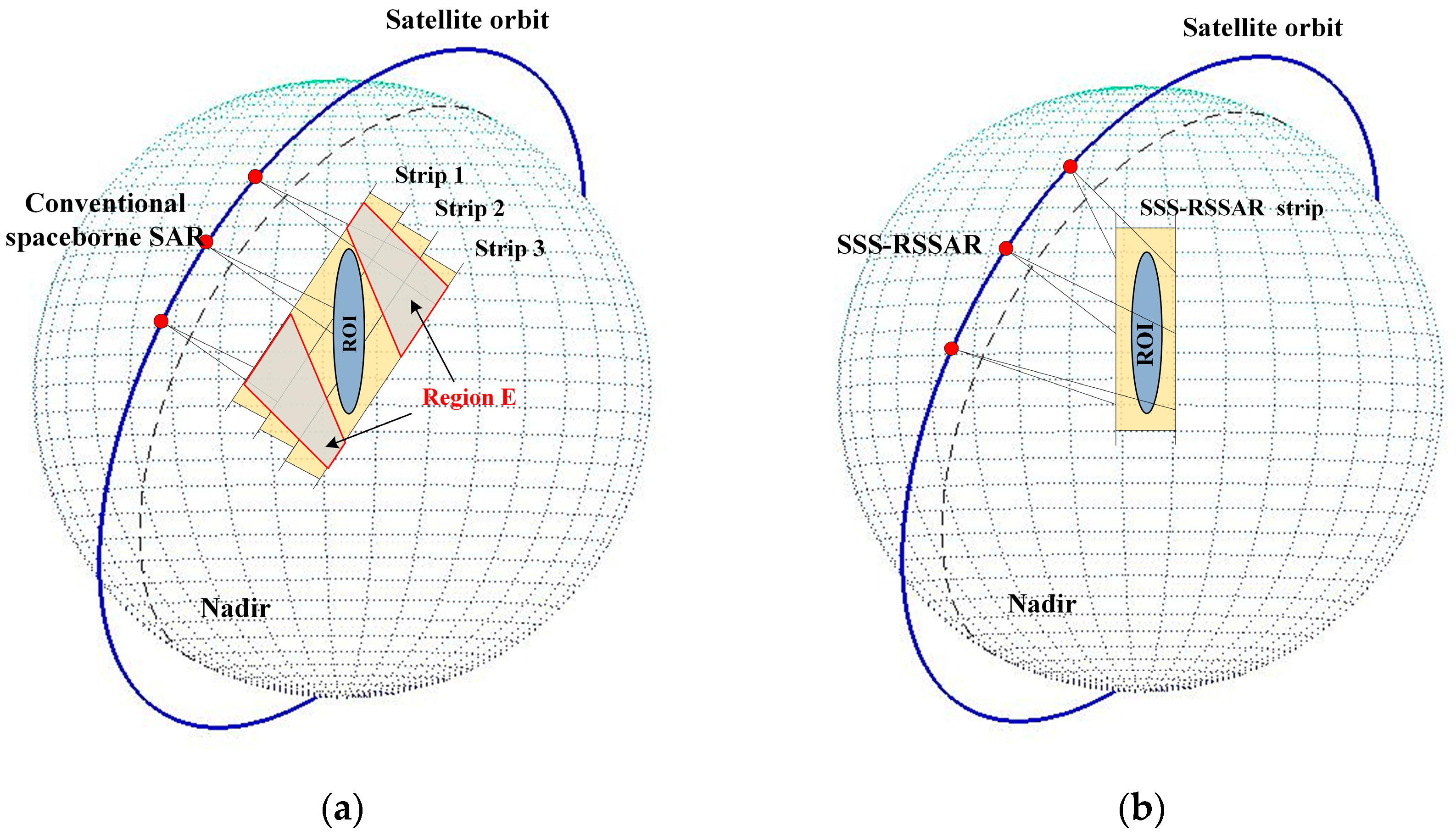
Figure 2.
SSS-RSSAR data acquisition geometry.

Figure 3.
Expected Continuous Varying Pulse Interval (CVPI) based echo distribution.
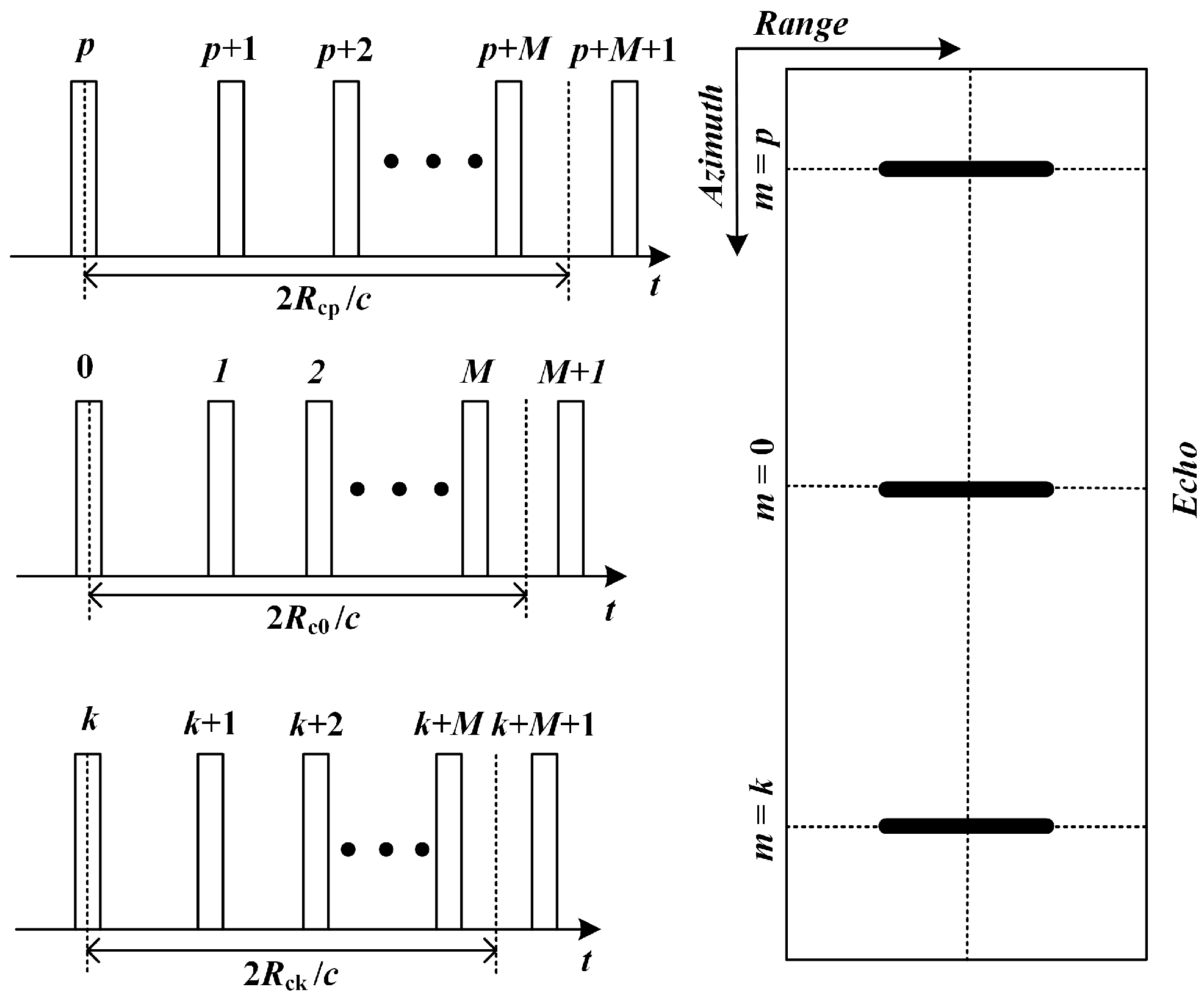
Figure 4.
Echoes before and after the zero padding if processed by the algorithms such as the Range Doppler Algorithm (RDA), Chirp Scaling Algorithm (CSA) and Range Migration Algorithm (RMA).
Figure 4.
Echoes before and after the zero padding if processed by the algorithms such as the Range Doppler Algorithm (RDA), Chirp Scaling Algorithm (CSA) and Range Migration Algorithm (RMA).

Figure 5.
Wavenumber data distributed in: (a) polar format; (b) keystone format; and (c) rectangular format.
Figure 5.
Wavenumber data distributed in: (a) polar format; (b) keystone format; and (c) rectangular format.

Figure 6.
Wavenumber data distributed in: (a) polar format; (b) keystone format; and (c) rectangular format when employing the new parameter adjusting manipulation.
Figure 6.
Wavenumber data distributed in: (a) polar format; (b) keystone format; and (c) rectangular format when employing the new parameter adjusting manipulation.
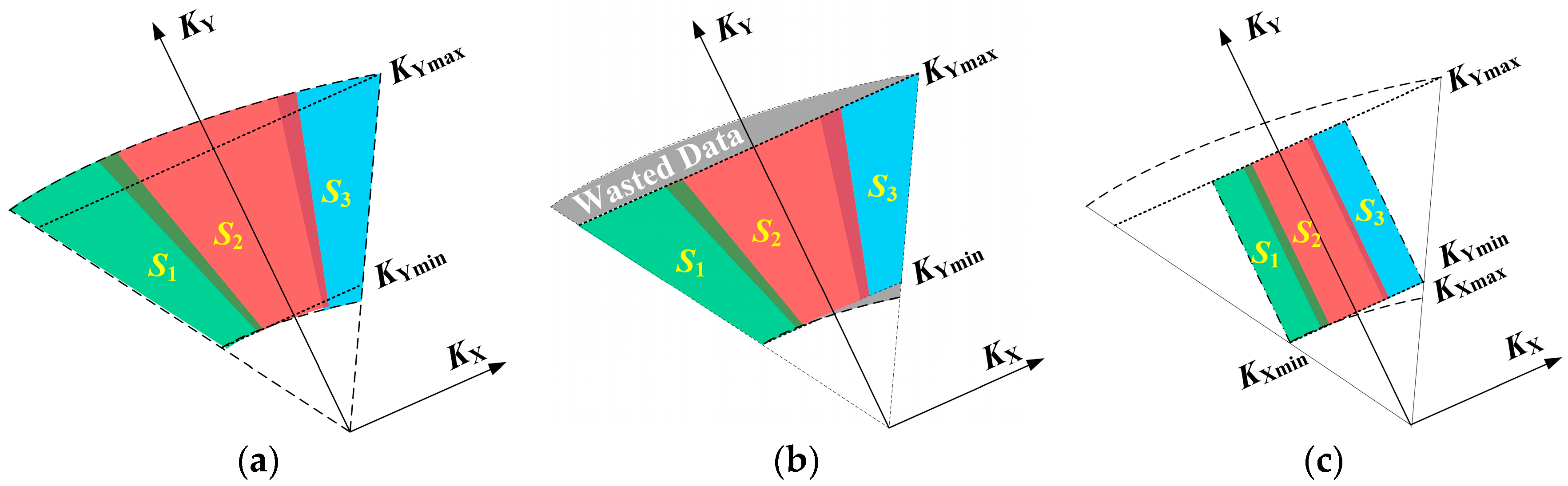
Figure 7.
Integrate system parameter design flowchart for the SSS-RSSAR.
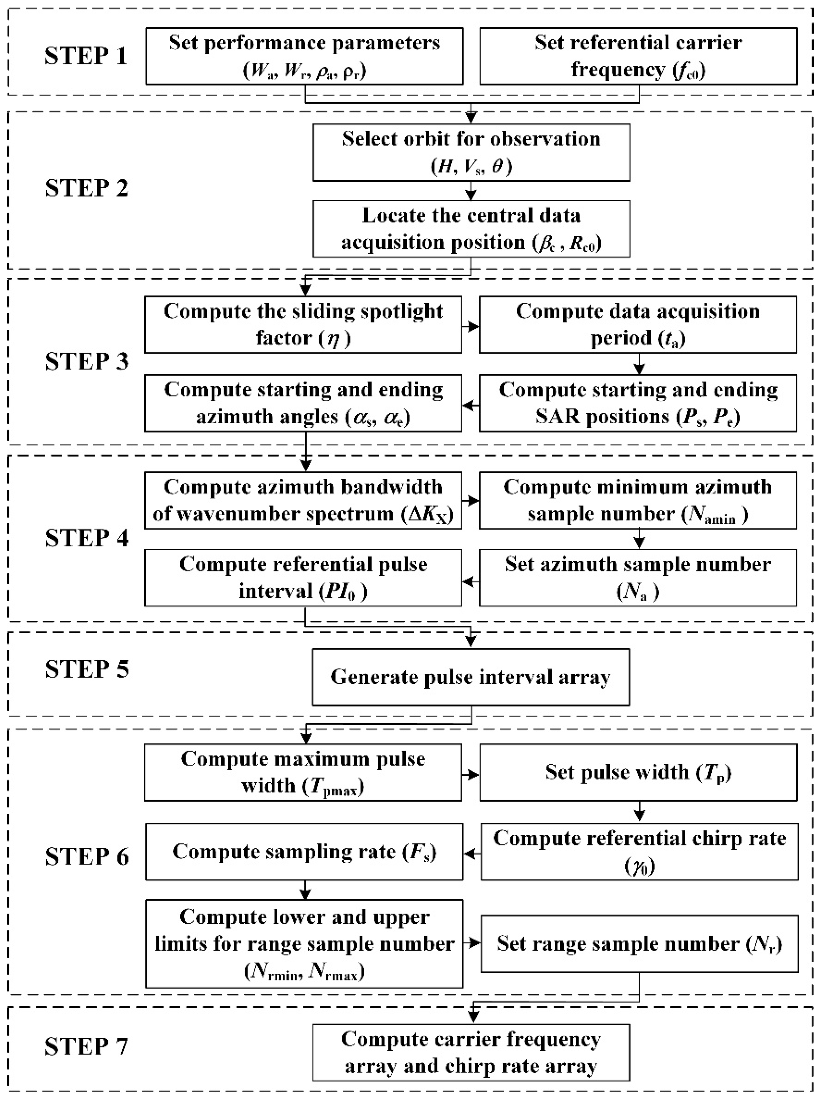
Figure 8.
Target distribution for the SSS-RSSAR simulation.
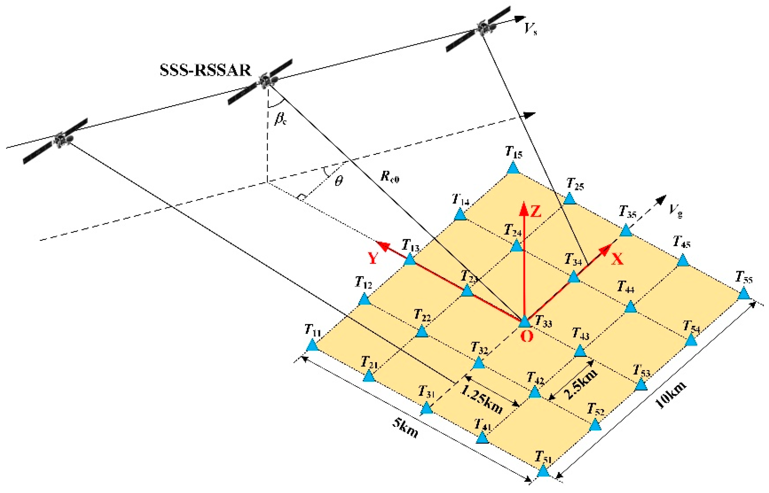
Figure 9.
Variations of: (a) CBSR; and (b) PI array with respect the azimuth time.
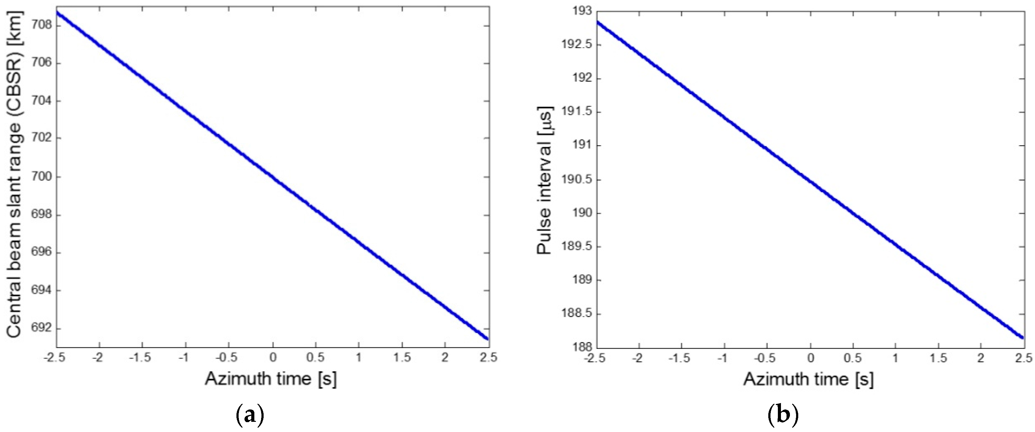
Figure 10.
Simulated echoes when: (a) using the CVPI technique; and (b) not using the CVPI technique. The white and black regions denote the valid data and no data, respectively.
Figure 10.
Simulated echoes when: (a) using the CVPI technique; and (b) not using the CVPI technique. The white and black regions denote the valid data and no data, respectively.
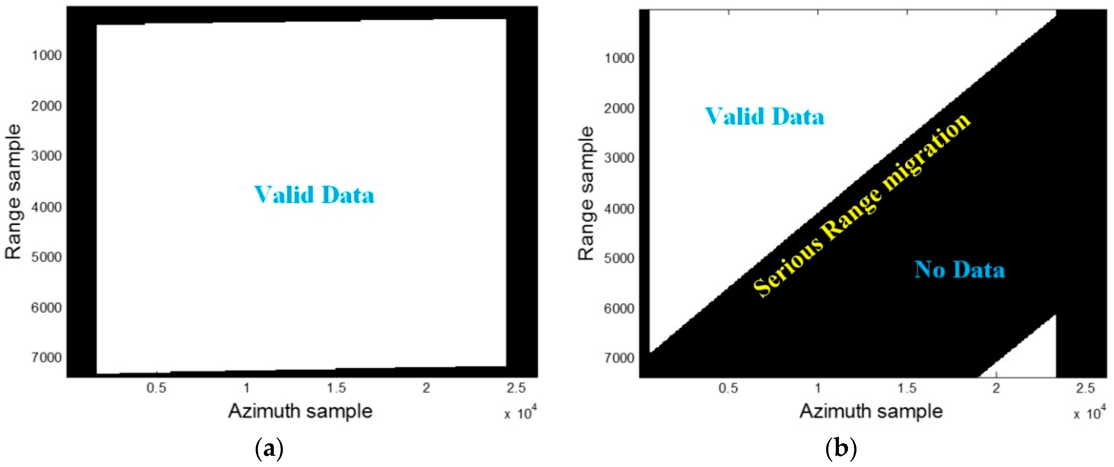
Figure 11.
Azimuth dependent: (a) carrier frequency; and (b) chirp rate when the new parameter adjusting technique is employed.
Figure 11.
Azimuth dependent: (a) carrier frequency; and (b) chirp rate when the new parameter adjusting technique is employed.
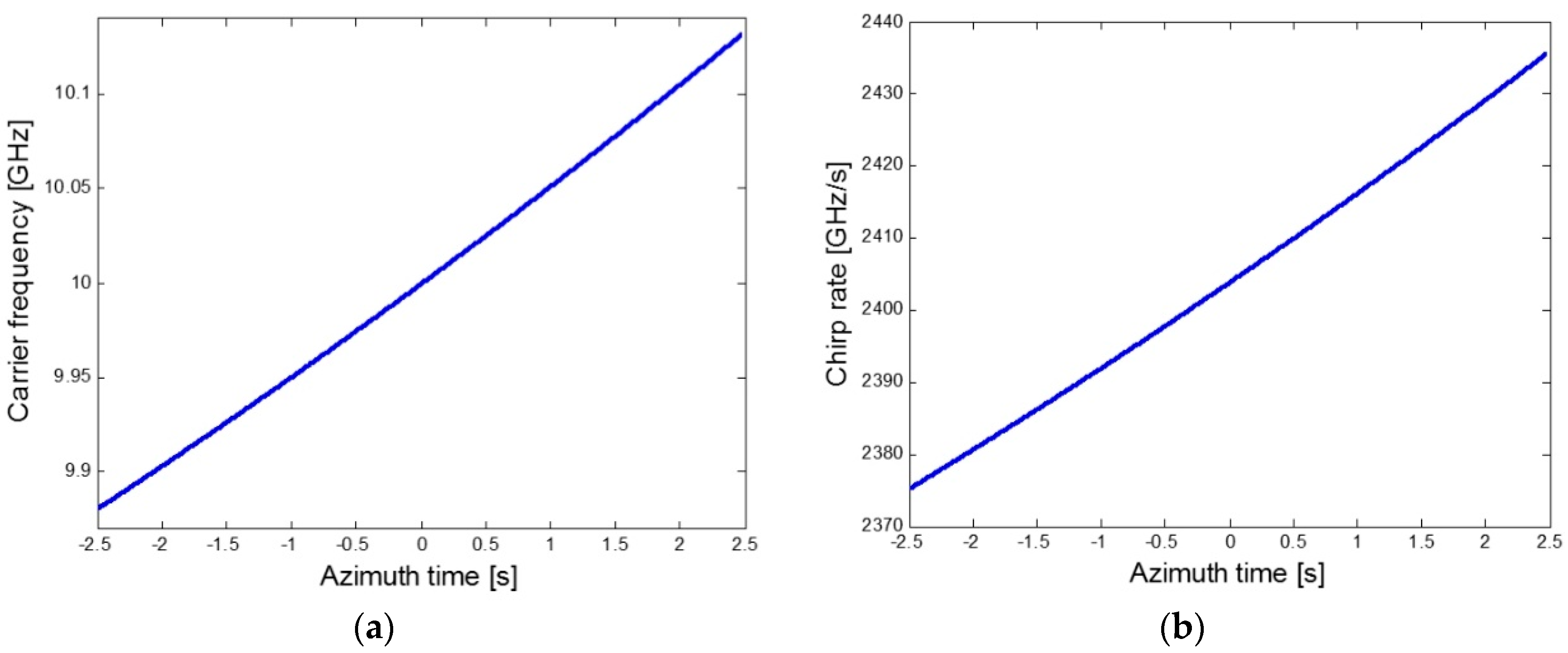
Figure 12.
Range wavenumber when: (a) using the parameter adjusting technique; and (b) not using the parameter adjusting technique.
Figure 12.
Range wavenumber when: (a) using the parameter adjusting technique; and (b) not using the parameter adjusting technique.
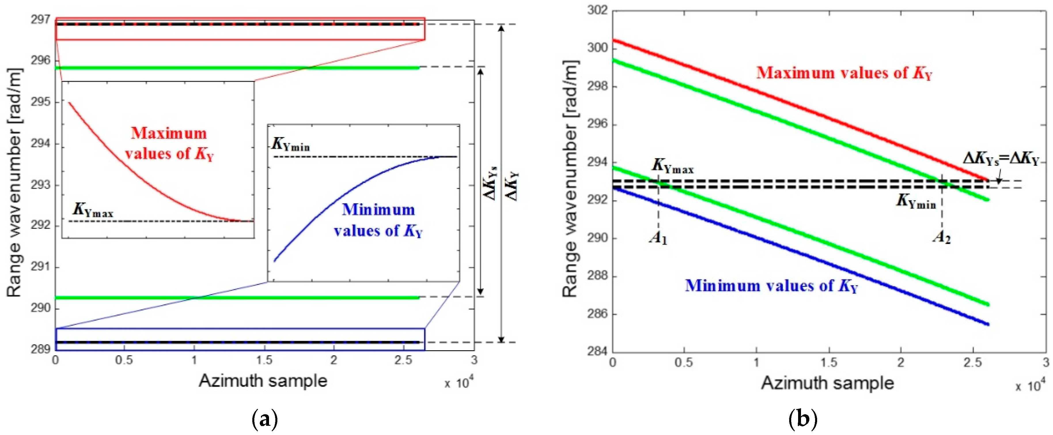
Figure 13.
Focusing performances of T33 when: (a) using the parameter adjusting technique; and (b) not using the parameter adjusting technique.
Figure 13.
Focusing performances of T33 when: (a) using the parameter adjusting technique; and (b) not using the parameter adjusting technique.
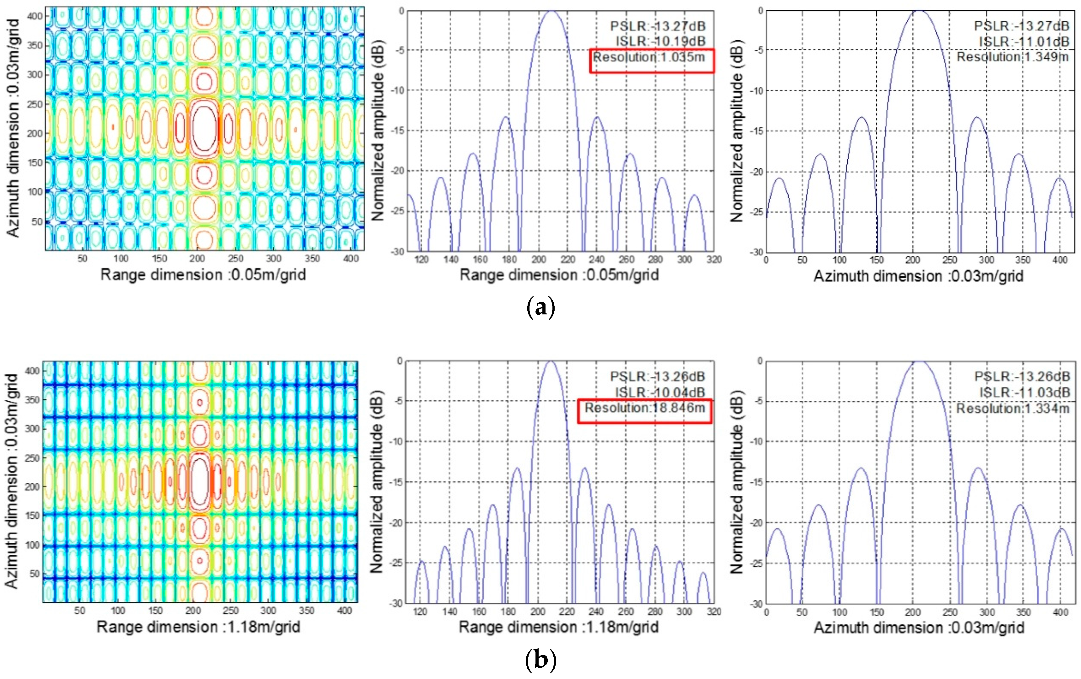
Figure 14.
Contour plots focused: (a) T11; (b) T13; (c) T15; (d) T31; (e) T33; (f) T35; (g) T51; (h) T53; and (i) T55 with the parameter adjusting technique.
Figure 14.
Contour plots focused: (a) T11; (b) T13; (c) T15; (d) T31; (e) T33; (f) T35; (g) T51; (h) T53; and (i) T55 with the parameter adjusting technique.

Figure 15.
Total sample number variation of: (a) SSS-RSSAR; and (b) traditional sliding spotlight SAR with respect to the ROI swath.
Figure 15.
Total sample number variation of: (a) SSS-RSSAR; and (b) traditional sliding spotlight SAR with respect to the ROI swath.
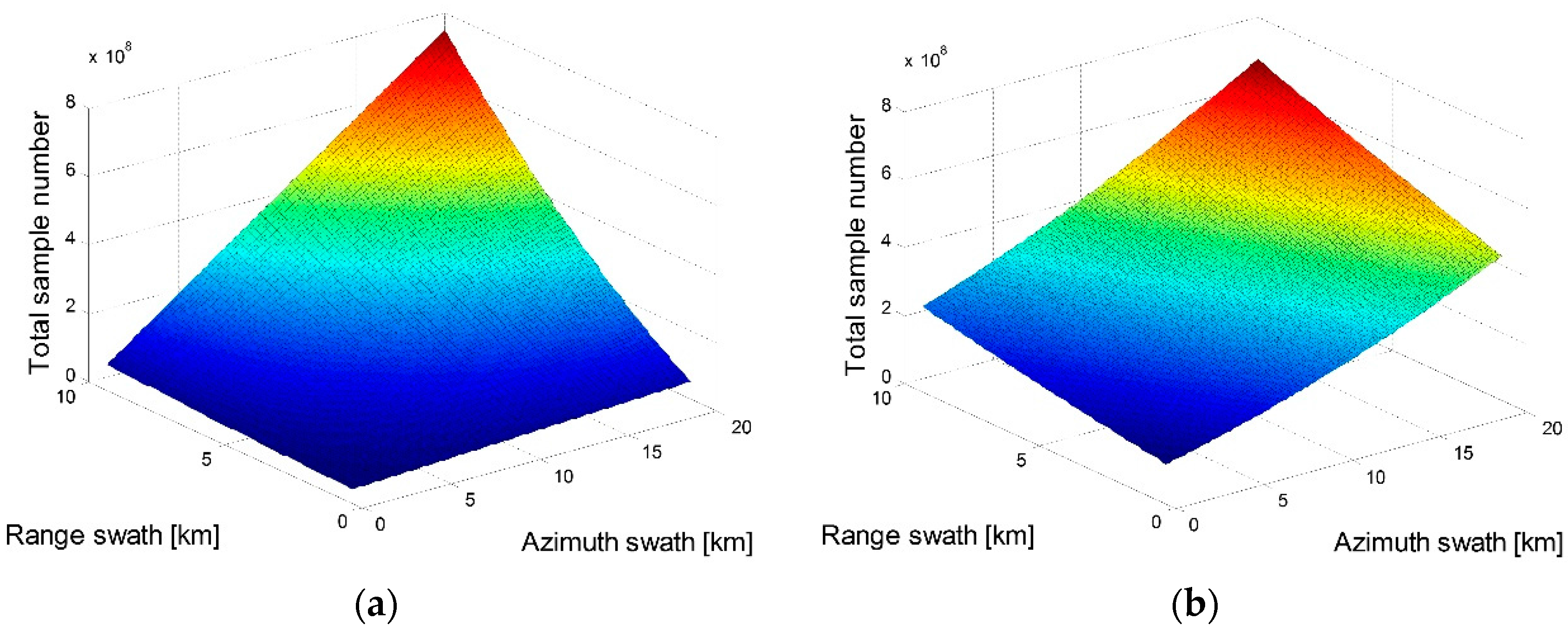
Figure 16.
Total computational loads of: (a) RDA; (b) CSA; (c) RMA; and (d) MPFA.

Table 1.
Computational load of basic operations.
| Basic Operation | Computational Load (In FLOP) |
|---|---|
| FFT/IFFT (N points) | 5Nlog2N |
| Complex multiply | 6 |
| Interpolation (Mk-point kernel) | 4Mk − 2 |
Table 2.
Computational load of the Modified Polar Format Algorithm (MPFA).
| Step | Operation | Computational Load (In FLOP) |
|---|---|---|
| 2D dechirping | Complex multiply (Fdechirp) | 6NaNr |
| RVP removal | Range FFT | 5NaNrlog2Nr |
| Complex multiply (FRVP) | 6NaNr | |
| Range IFFT | 5NaNrlog2Nr | |
| Data correction | Range interpolation (Mk-point kernel) | 2NaNr (2Mk − 1) |
| Azimuth interpolation (Mk-point kernel) | 2NaNr (2Mk − 1) | |
| Image generation | Range FFT | 5NaNrlog2Nr |
| Azimuth FFT | 5NaNrlog2Na | |
| Total computational load of the MPFA | 12NaNr + 4NaNr (2Mk − 1) + 15NaNrlog2Nr + 5NaNrlog2Na | |
Table 3.
Computational loads of classical imaging algorithms.
| Algorithms | Computational Load (In FLOP) |
|---|---|
| RDA | 12NaminTNrminT + 10NaminTNrminTlog2NaminT + 10NaminTNrminTlog2NrminT + 2NaminTNrminT (2Mk − 1) |
| CSA | 18NaminTNrminT + 10NaminTNrminTlog2NaminT + 10NaminTNrminTlog2NrminT |
| RMA | 6NaminTNrminT + 10NaminTNrminTlog2NaminT + 10NaminTNrminTlog2NrminT + 2NaminTNrminT (2Mk − 1) |
Table 4.
Key parameters for the SSS-RSSAR simulation.
| Step | Parameter | Value |
|---|---|---|
| Basic Parameters | Referential carrier frequency fc0 | 10 GHz |
| Platform velocity Vs | 7 km/s | |
| Platform height H | 500 km | |
| Antenna beam width ϕa | 0.41° | |
| Tilt angle θ | 45.0° | |
| Central look angle βc0 | 44.4° | |
| Central slant range Rc0 | 700 km | |
| ROI swath (Wr × Wa) | 5 km × 10 km | |
| Resolution (ρr × ρa) | 1.00 m × 1.31 m | |
| Derived Parameters | Sliding Spotlight factor η | 0.7 |
| Bandwidth Br | 189.9 MHz | |
| Pulse width Tp | 79.0 μs | |
| Referential chirp rate γ0 | 2404 GHz/s | |
| Sampling rate Fs | 67.3 MHz | |
| Referential pulse interval PI0 | 192.8 μs | |
| Sample number (Nr × Na) | 7344 × 26,124 |
Table 5.
Focusing quality evaluation.
| T11 | T13 | T15 | T31 | T33 | T35 | T51 | T53 | T55 | ||
|---|---|---|---|---|---|---|---|---|---|---|
| Range | PSLR (dB) | −13.25 | −13.26 | −13.25 | −13.21 | −13.27 | −13.26 | −13.23 | −13.27 | −13.29 |
| ISLR (dB) | −10.20 | −10.18 | −10.22 | −10.21 | −10.19 | −10.18 | −10.23 | −10.18 | −10.23 | |
| Res. (m) | 1.035 | 1.035 | 1.035 | 1.035 | 1.035 | 1.035 | 1.035 | 1.035 | 1.035 | |
| Azimuth | PSLR (dB) | −13.24 | −13.26 | −13.16 | −13.21 | −13.27 | −13.16 | −13.16 | −13.25 | −13.18 |
| ISLR (dB) | −11.02 | −11.00 | −10.65 | −10.98 | −11.01 | −10.91 | −10.73 | −11.00 | −10.63 | |
| Res. (m) | 1.376 | 1.349 | 1.332 | 1.376 | 1.349 | 1.295 | 1.365 | 1.349 | 1.298 |
© 2017 by the authors. Licensee MDPI, Basel, Switzerland. This article is an open access article distributed under the terms and conditions of the Creative Commons Attribution (CC BY) license (http://creativecommons.org/licenses/by/4.0/).
Share and Cite
MDPI and ACS Style
Wang, Y.; Li, J.; Yang, J.; Sun, B. A Novel Spaceborne Sliding Spotlight Range Sweep Synthetic Aperture Radar: System and Imaging. Remote Sens. 2017, 9, 783. https://doi.org/10.3390/rs9080783
AMA Style
Wang Y, Li J, Yang J, Sun B. A Novel Spaceborne Sliding Spotlight Range Sweep Synthetic Aperture Radar: System and Imaging. Remote Sensing. 2017; 9(8):783. https://doi.org/10.3390/rs9080783
Chicago/Turabian StyleWang, Yan, Jingwen Li, Jian Yang, and Bing Sun. 2017. "A Novel Spaceborne Sliding Spotlight Range Sweep Synthetic Aperture Radar: System and Imaging" Remote Sensing 9, no. 8: 783. https://doi.org/10.3390/rs9080783
Note that from the first issue of 2016, this journal uses article numbers instead of page numbers. See further details here.