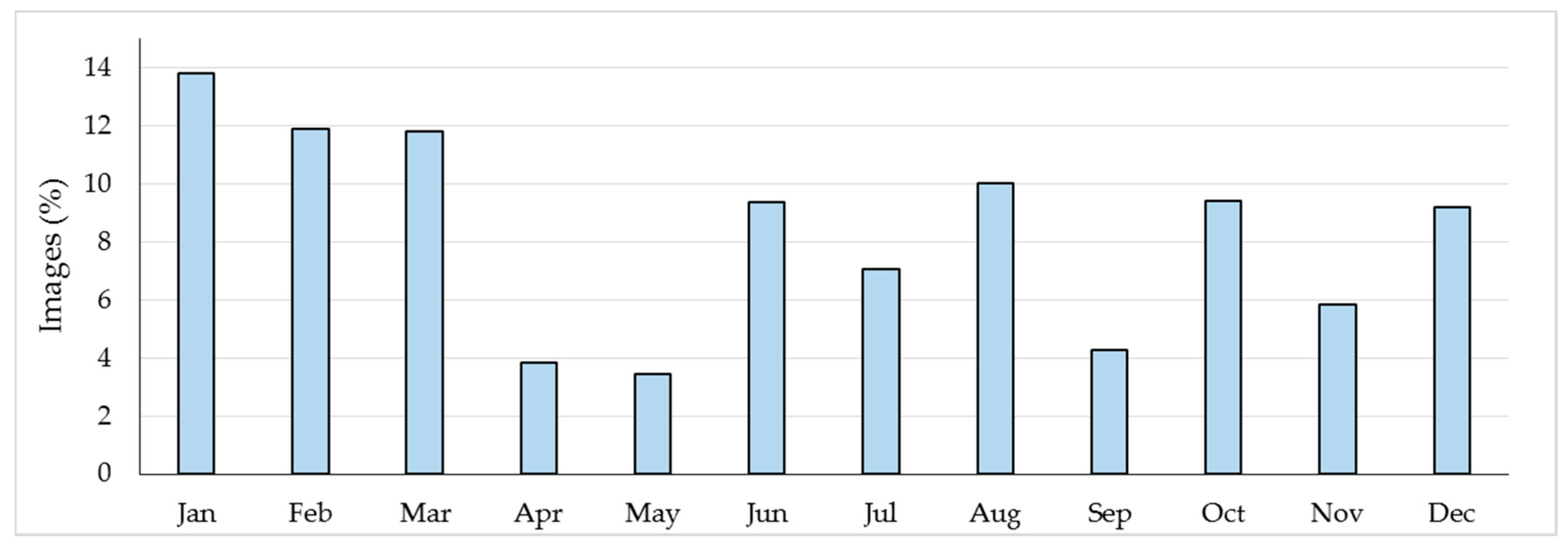
Figure 1.
Monthly distribution of very high resolution (VHR) imagery that was used during the data collection campaign.
Figure 1.
Monthly distribution of very high resolution (VHR) imagery that was used during the data collection campaign.
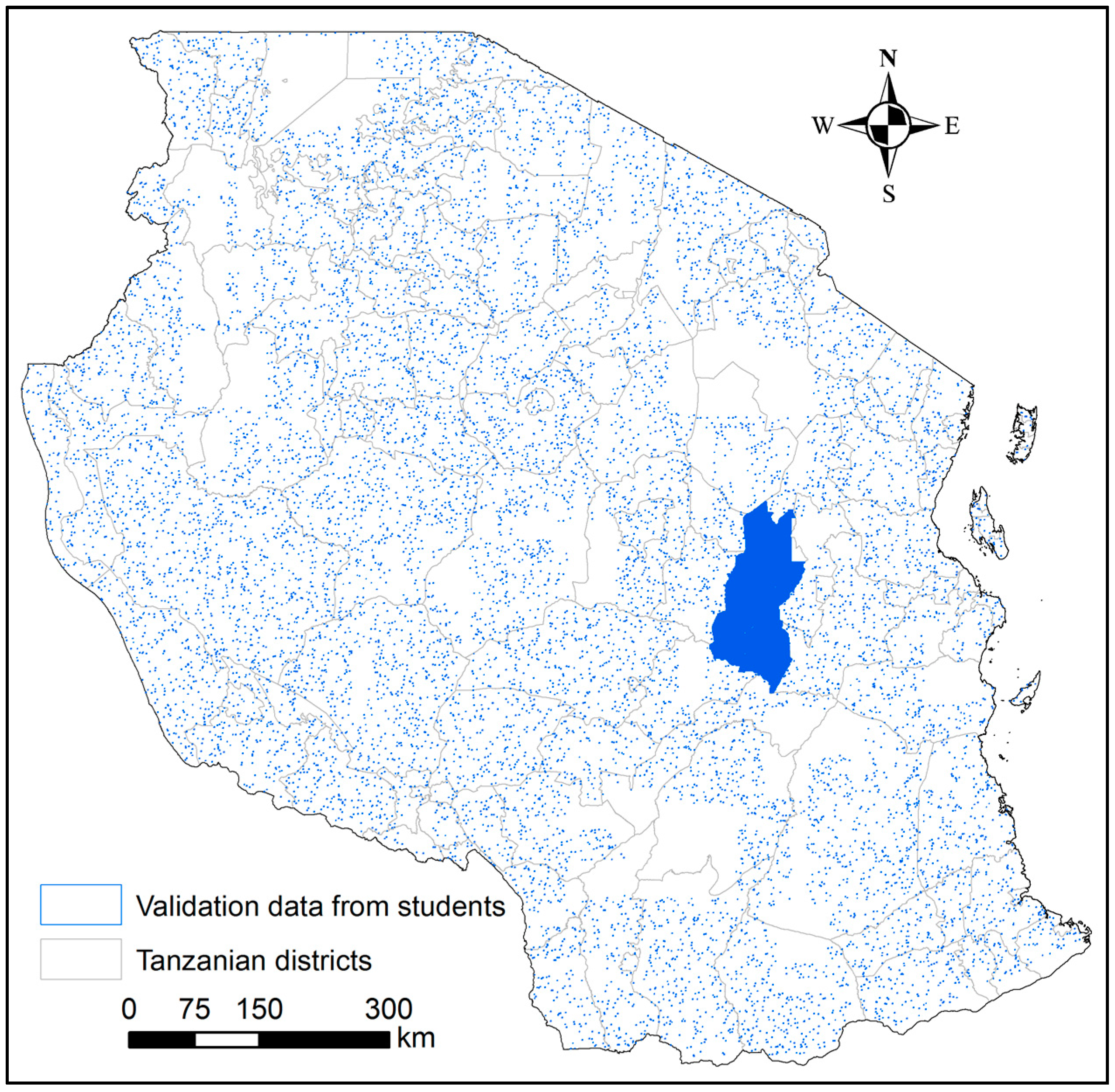
Figure 2.
Location and distribution of data collected across Tanzania with full coverage (wall-to-wall) in the Kilosa district.
Figure 2.
Location and distribution of data collected across Tanzania with full coverage (wall-to-wall) in the Kilosa district.
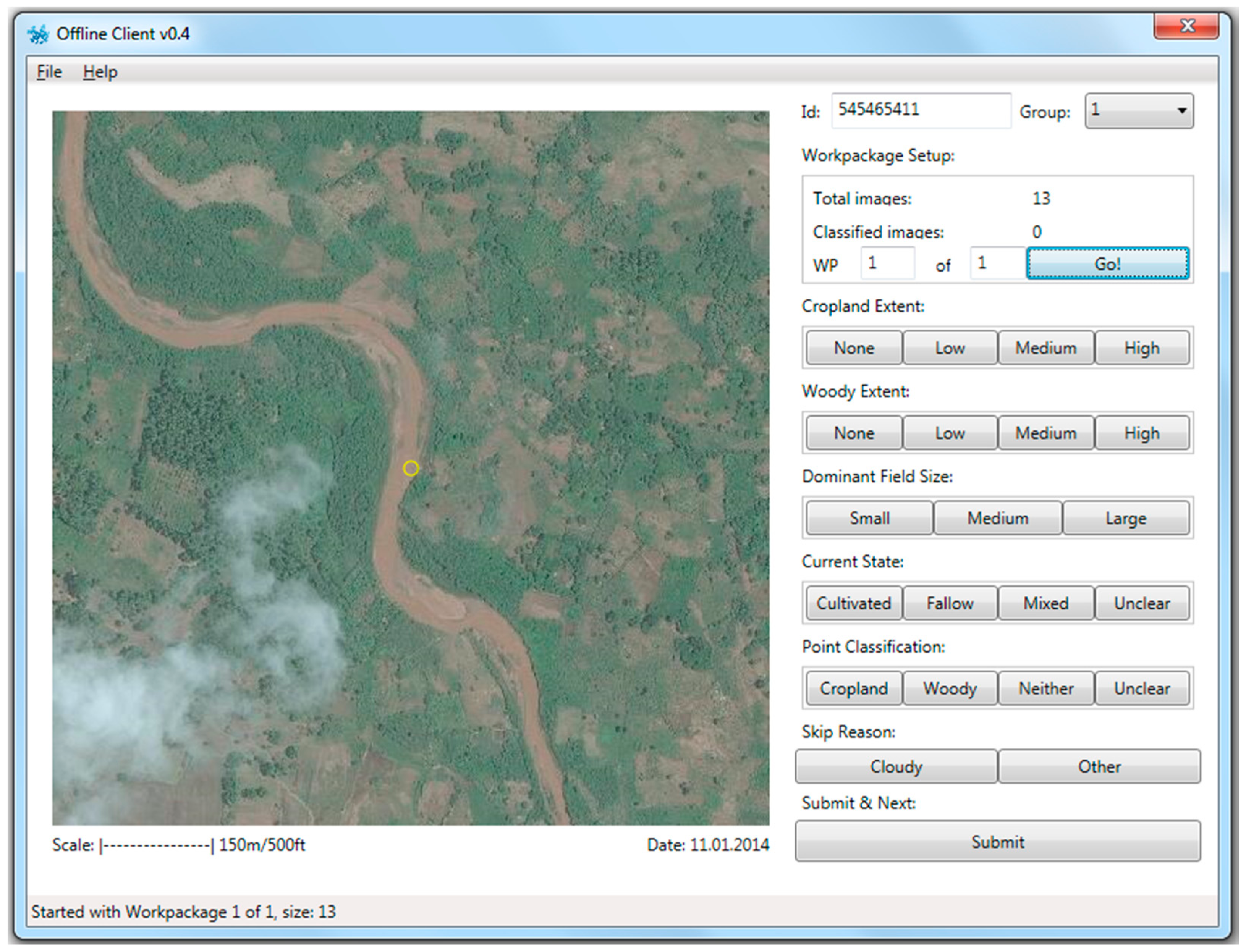
Figure 3.
The Geo-Wiki offline interface for collecting data on cropland and woodland extent.
Figure 3.
The Geo-Wiki offline interface for collecting data on cropland and woodland extent.
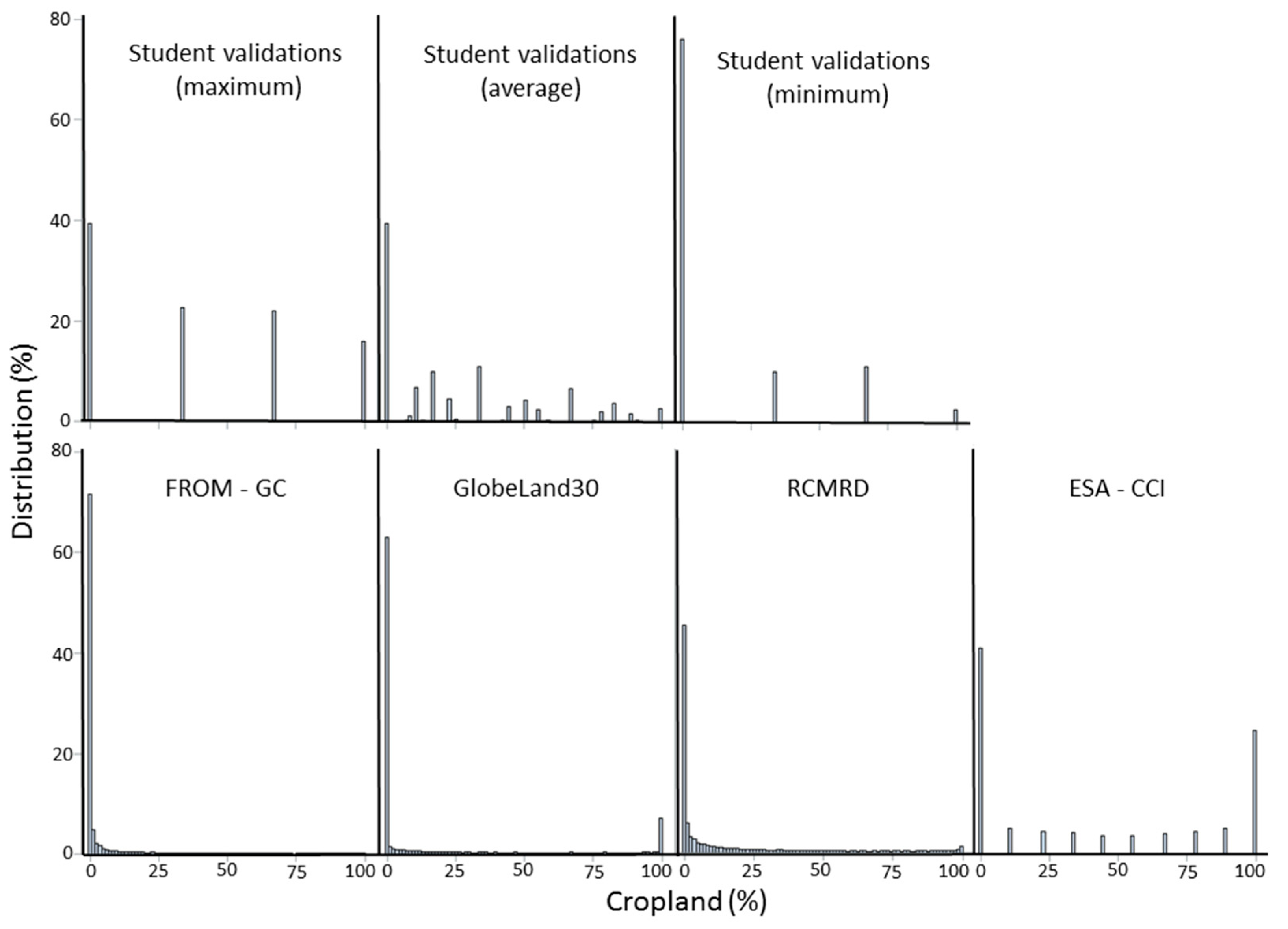
Figure 4.
Histograms of all data sets compared showing percentage cropland in the 1 × 1 km areas.
Figure 4.
Histograms of all data sets compared showing percentage cropland in the 1 × 1 km areas.
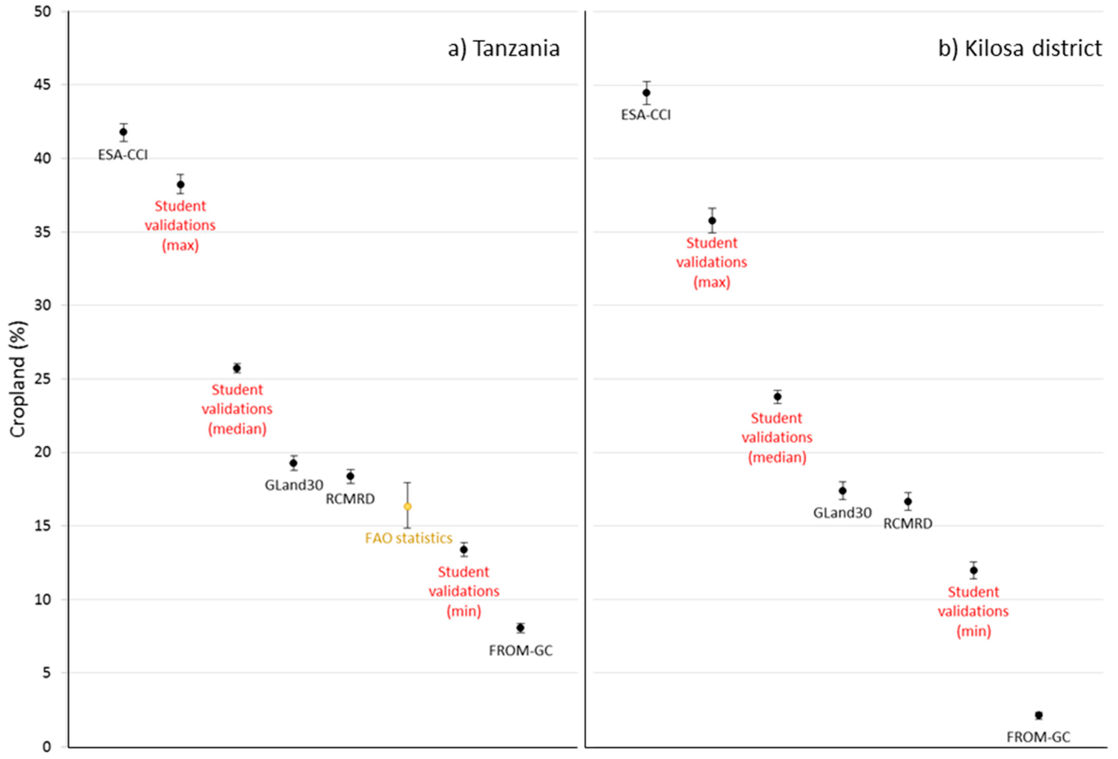
Figure 5.
Average (median) cropland (%) with bars showing upper and lower 95% confidence limits for (a) Tanzania (N obs = 170,296, N unique scenes = 25,935) and (b) Kilosa district (N obs = 95,251, N unique scenes = 14,533), sorted from highest to lowest. FAO statistics for Tanzania are included as a reference showing the mean (in yellow), as well as the minimum and maximum values for the years 2008 to 2014.
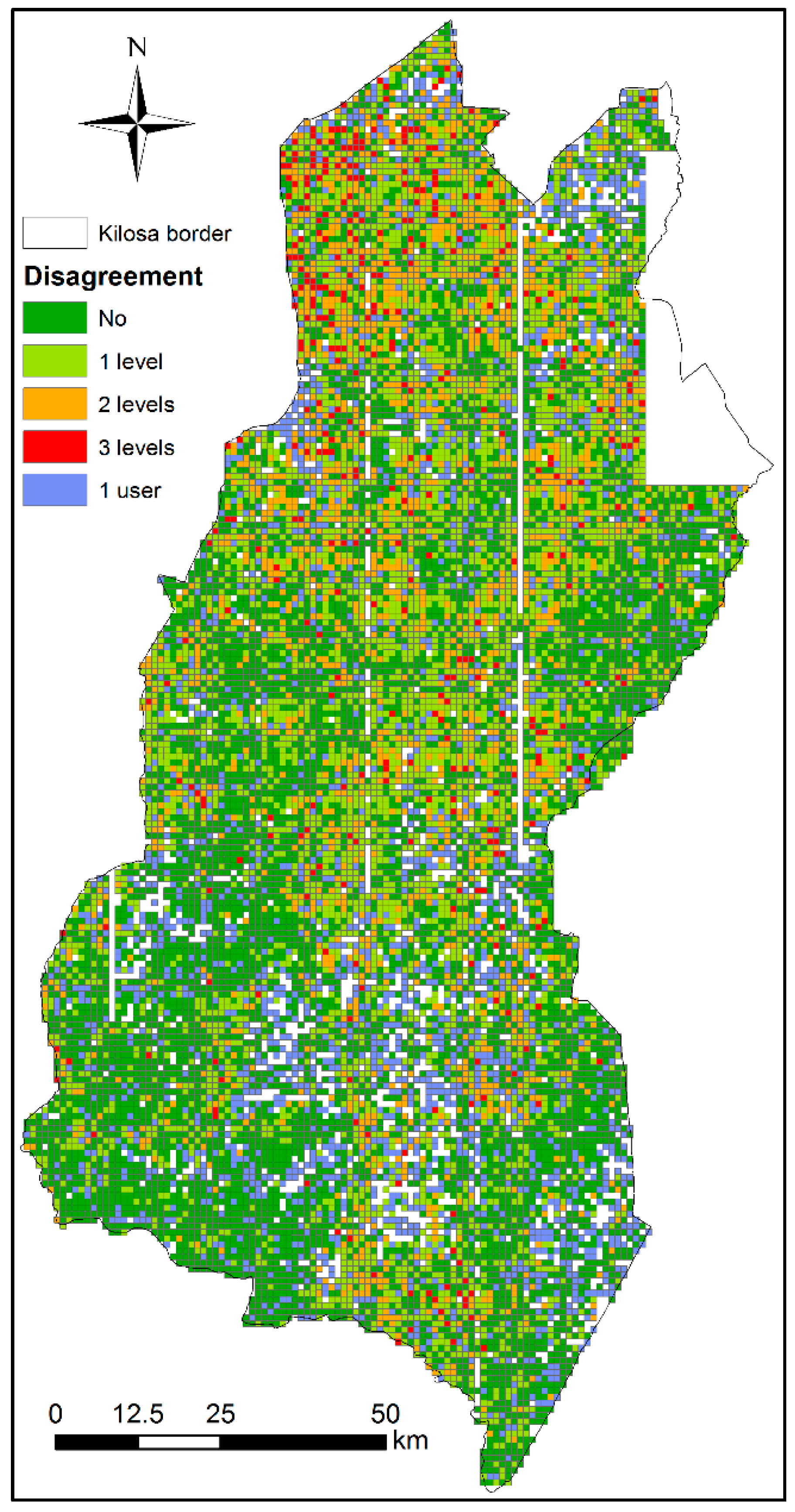
Figure 6.
Cropland disagreement between the student interpreters for the Kilosa district, Tanzania.
Figure 6.
Cropland disagreement between the student interpreters for the Kilosa district, Tanzania.
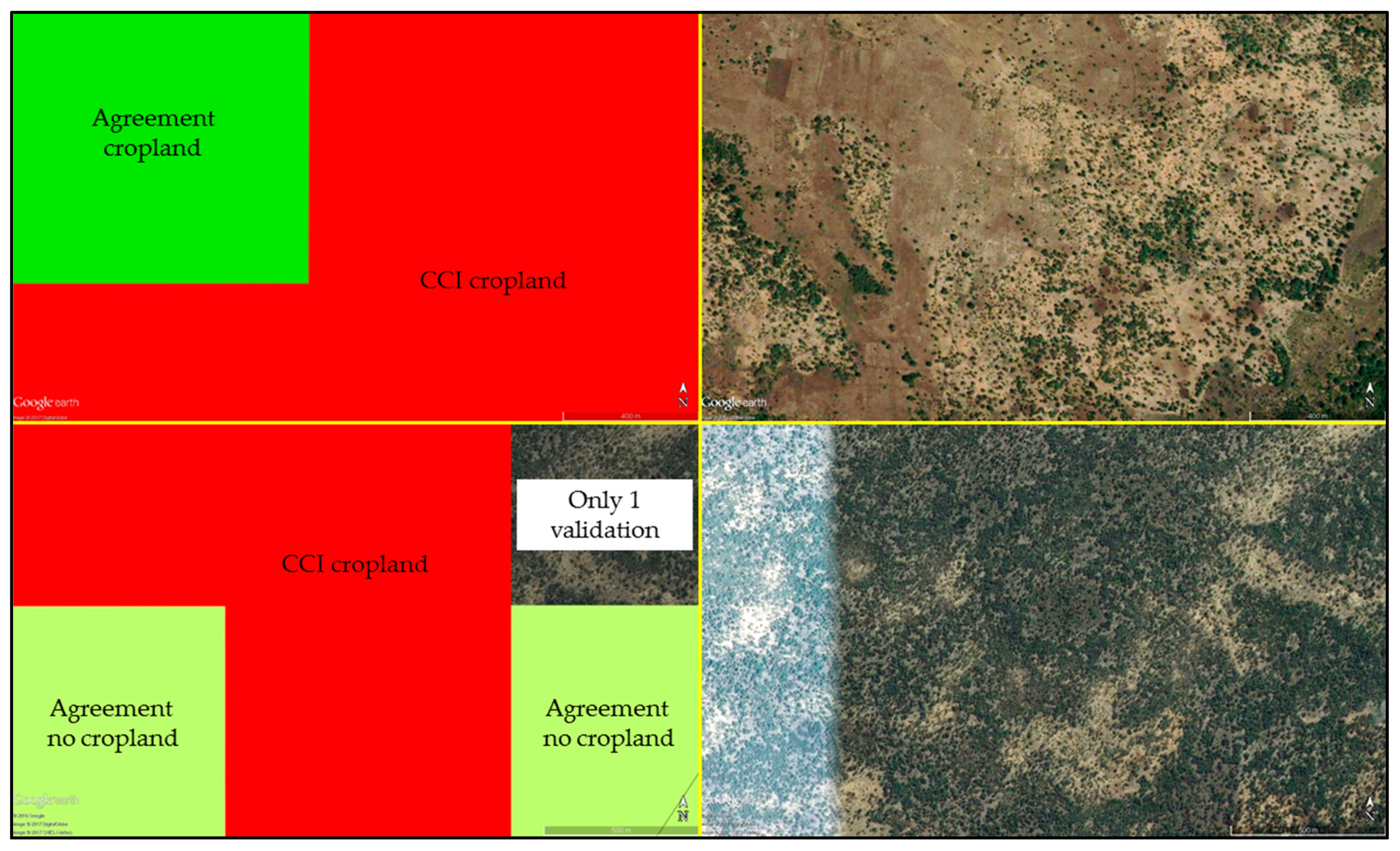
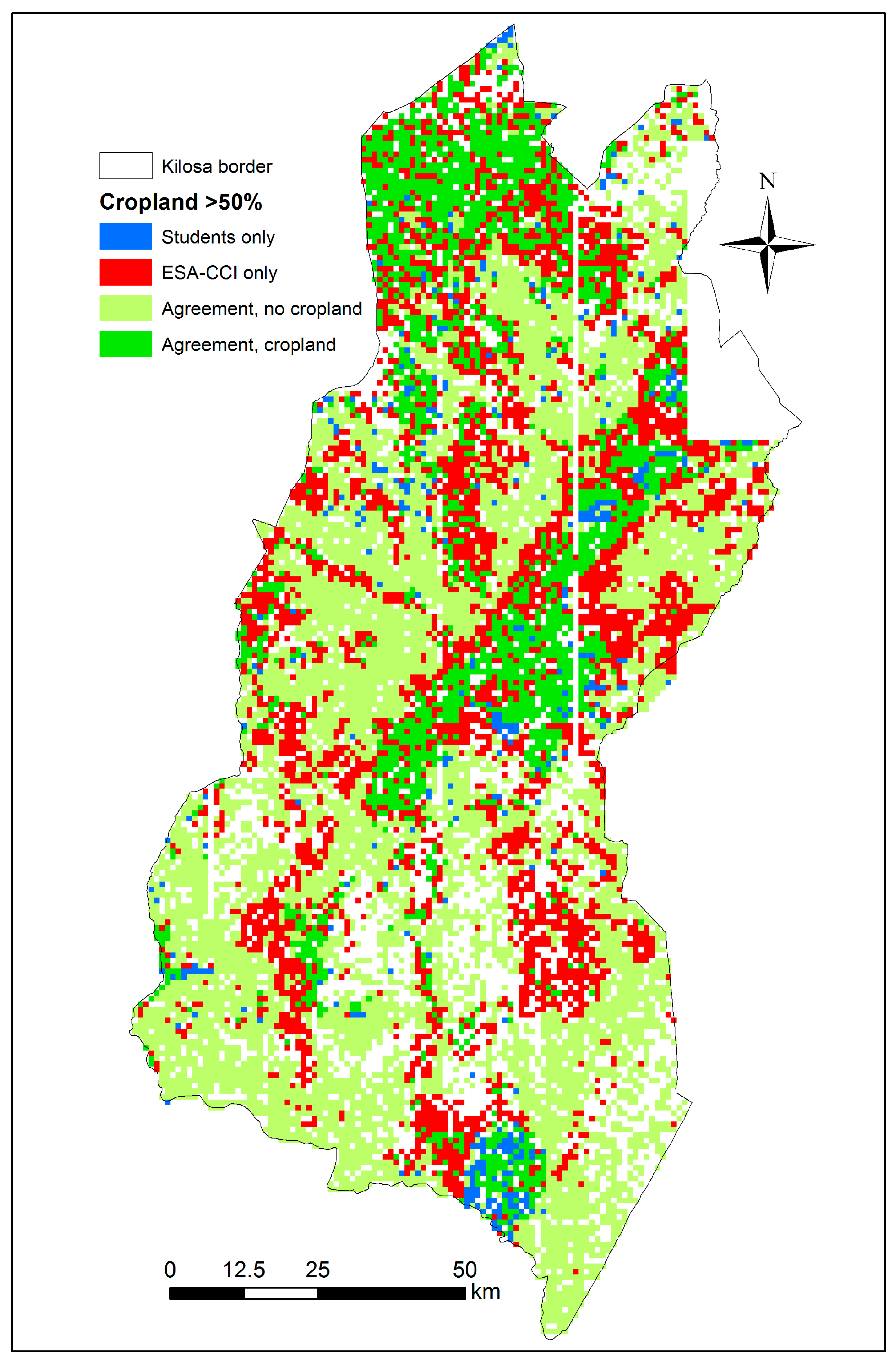
Figure 7.
Disagreement between the student validation and ESA-CCI data sets in the Kilosa district where each scene is considered as cropland if it has an average of more than 50% cropland (N = 12,373). A total of 2160 scenes have only one student interpretation and are shown as blank spaces.
Figure 7.
Disagreement between the student validation and ESA-CCI data sets in the Kilosa district where each scene is considered as cropland if it has an average of more than 50% cropland (N = 12,373). A total of 2160 scenes have only one student interpretation and are shown as blank spaces.
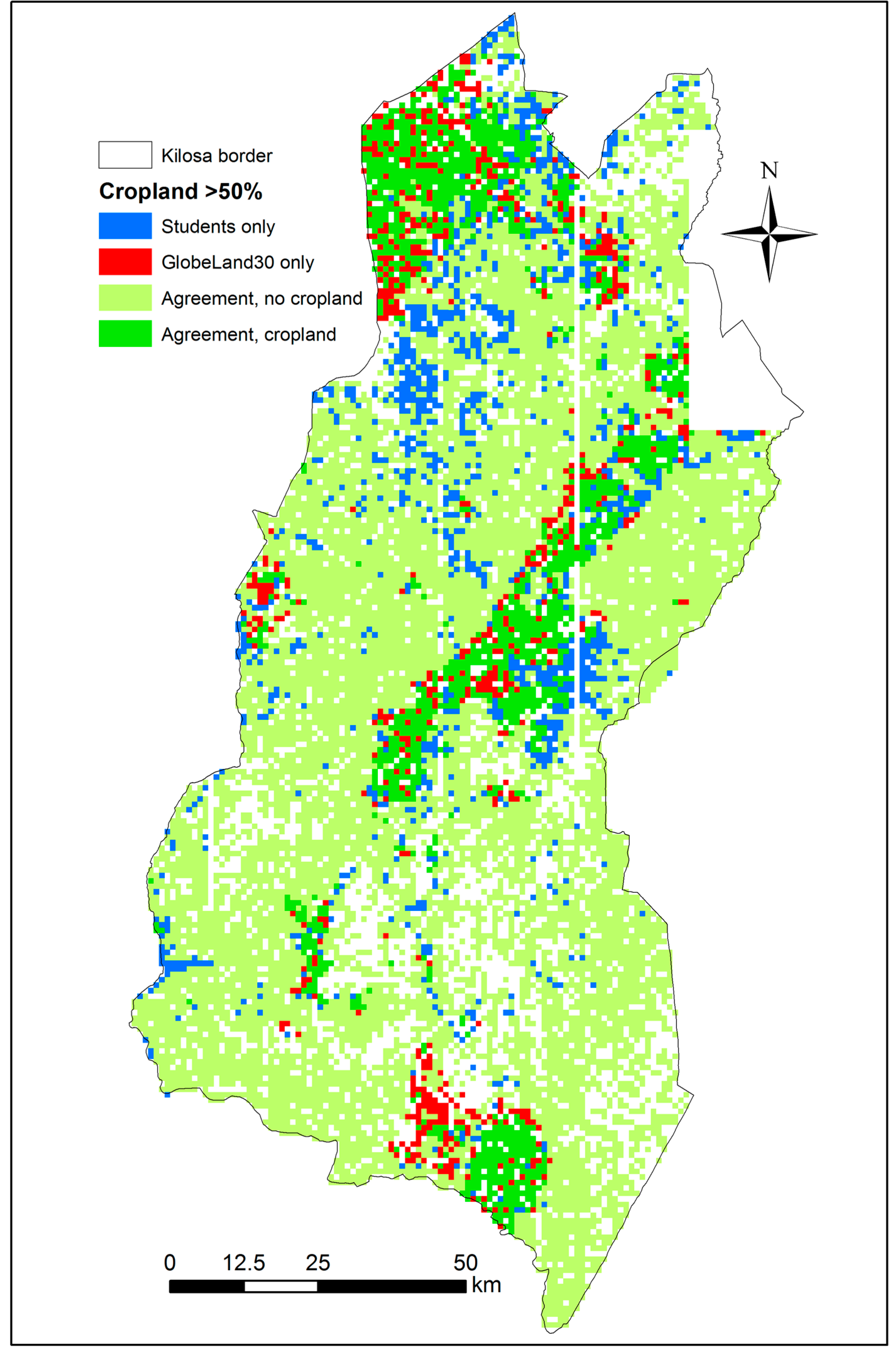
Figure 8.
Disagreement between the student validation and GlobeLand30 data sets in the Kilosa district where each scene is considered as cropland if it has an average of more than 50% cropland (N = 12,373). A total of 2160 scenes have only one student interpretation and are shown as blank spaces.
Figure 8.
Disagreement between the student validation and GlobeLand30 data sets in the Kilosa district where each scene is considered as cropland if it has an average of more than 50% cropland (N = 12,373). A total of 2160 scenes have only one student interpretation and are shown as blank spaces.
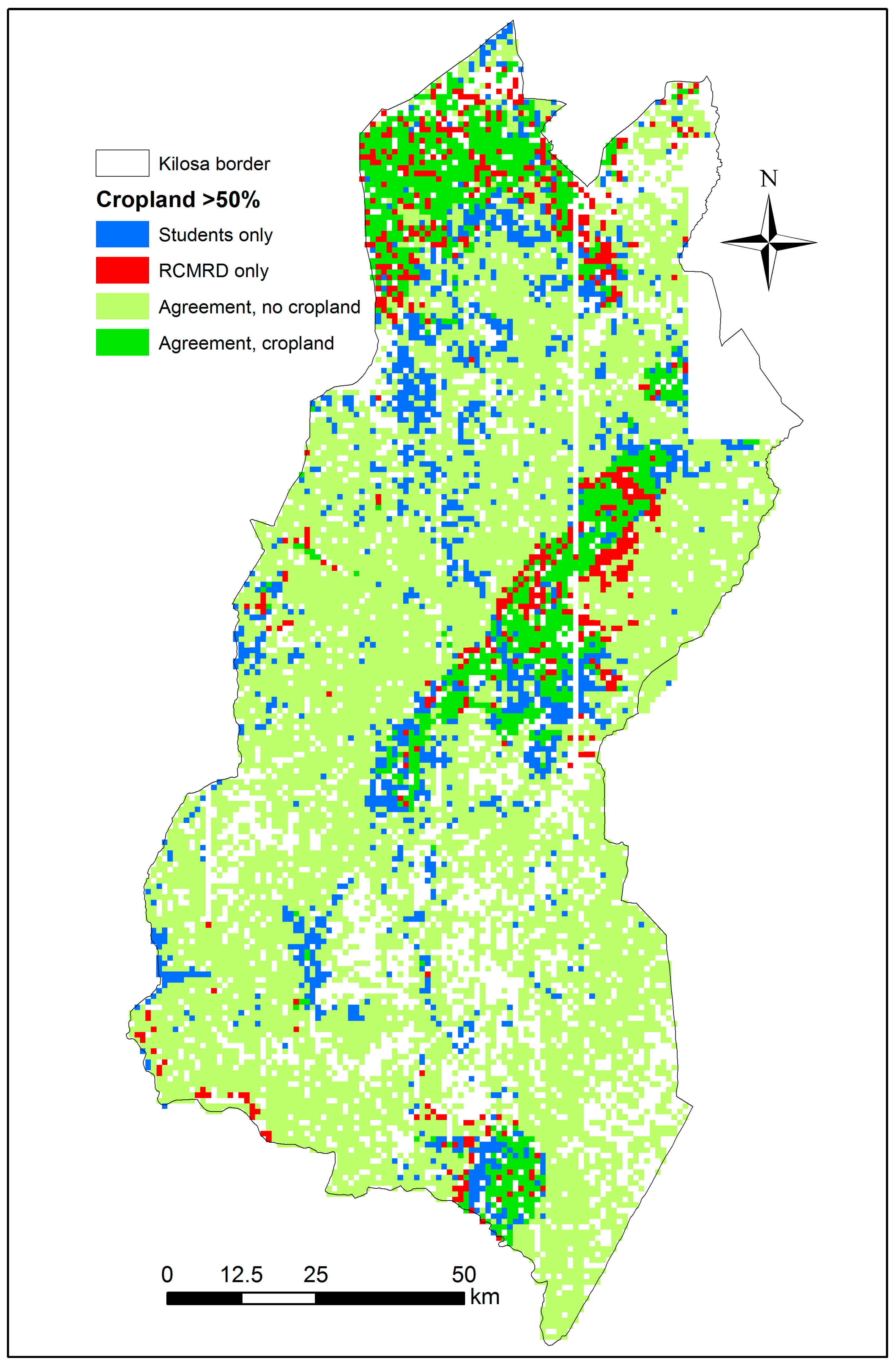
Figure 9.
Disagreement between the student validation and RCMRD data sets in the Kilosa district where each scene is considered as cropland if it has an average of more than 50% cropland (N = 12,373). A total of 2160 scenes have only one student interpretation and are shown as blank spaces.
Figure 9.
Disagreement between the student validation and RCMRD data sets in the Kilosa district where each scene is considered as cropland if it has an average of more than 50% cropland (N = 12,373). A total of 2160 scenes have only one student interpretation and are shown as blank spaces.
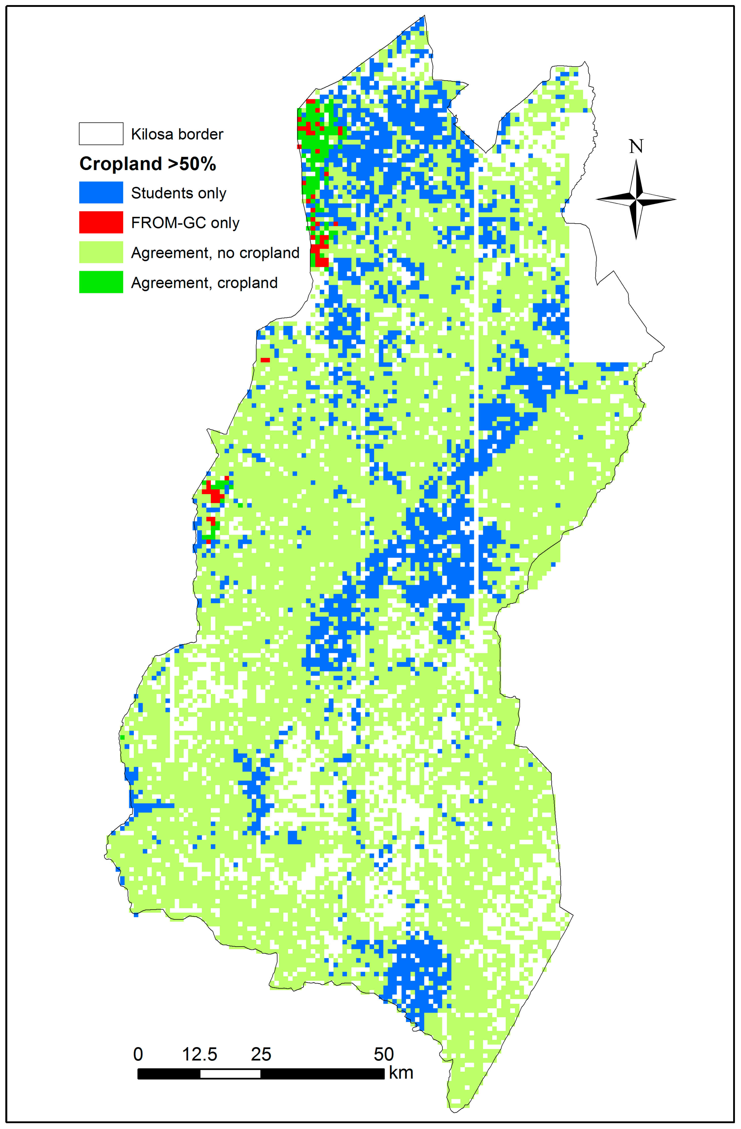
Figure 10.
Disagreement between the student validation and FROM-GC data sets in the Kilosa district where each scene is considered as cropland if it has an average of more than 50% cropland (N = 12,373). A total of 2160 scenes have only one student interpretation and are shown as blank spaces.
Figure 10.
Disagreement between the student validation and FROM-GC data sets in the Kilosa district where each scene is considered as cropland if it has an average of more than 50% cropland (N = 12,373). A total of 2160 scenes have only one student interpretation and are shown as blank spaces.
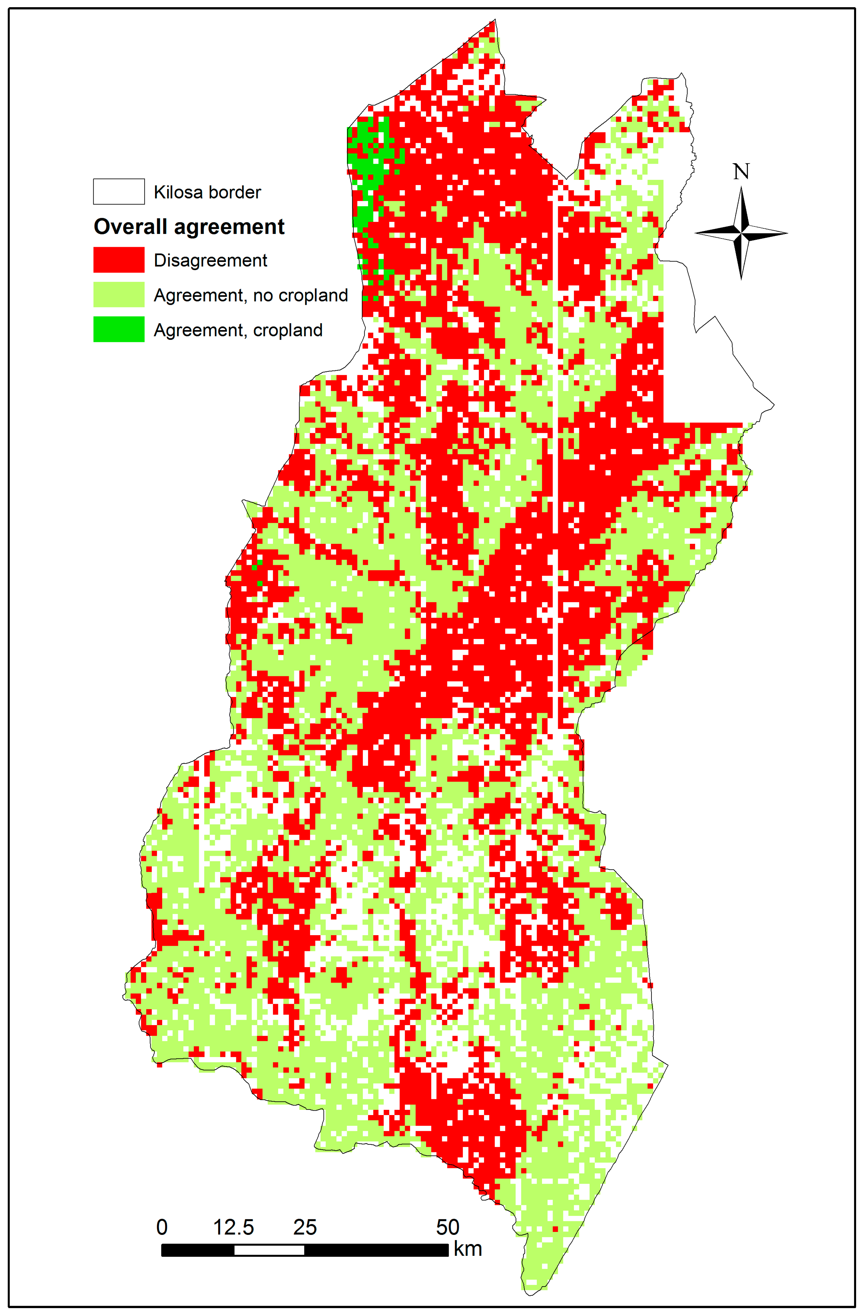
Figure 11.
Overall agreement across all cropland data sets in the Kilosa district where a given scene is considered as cropland if it has an average of more than 50% cropland (N = 12,373). A total of 2160 scenes have only one student interpretation and are shown as blank spaces.
Figure 11.
Overall agreement across all cropland data sets in the Kilosa district where a given scene is considered as cropland if it has an average of more than 50% cropland (N = 12,373). A total of 2160 scenes have only one student interpretation and are shown as blank spaces.
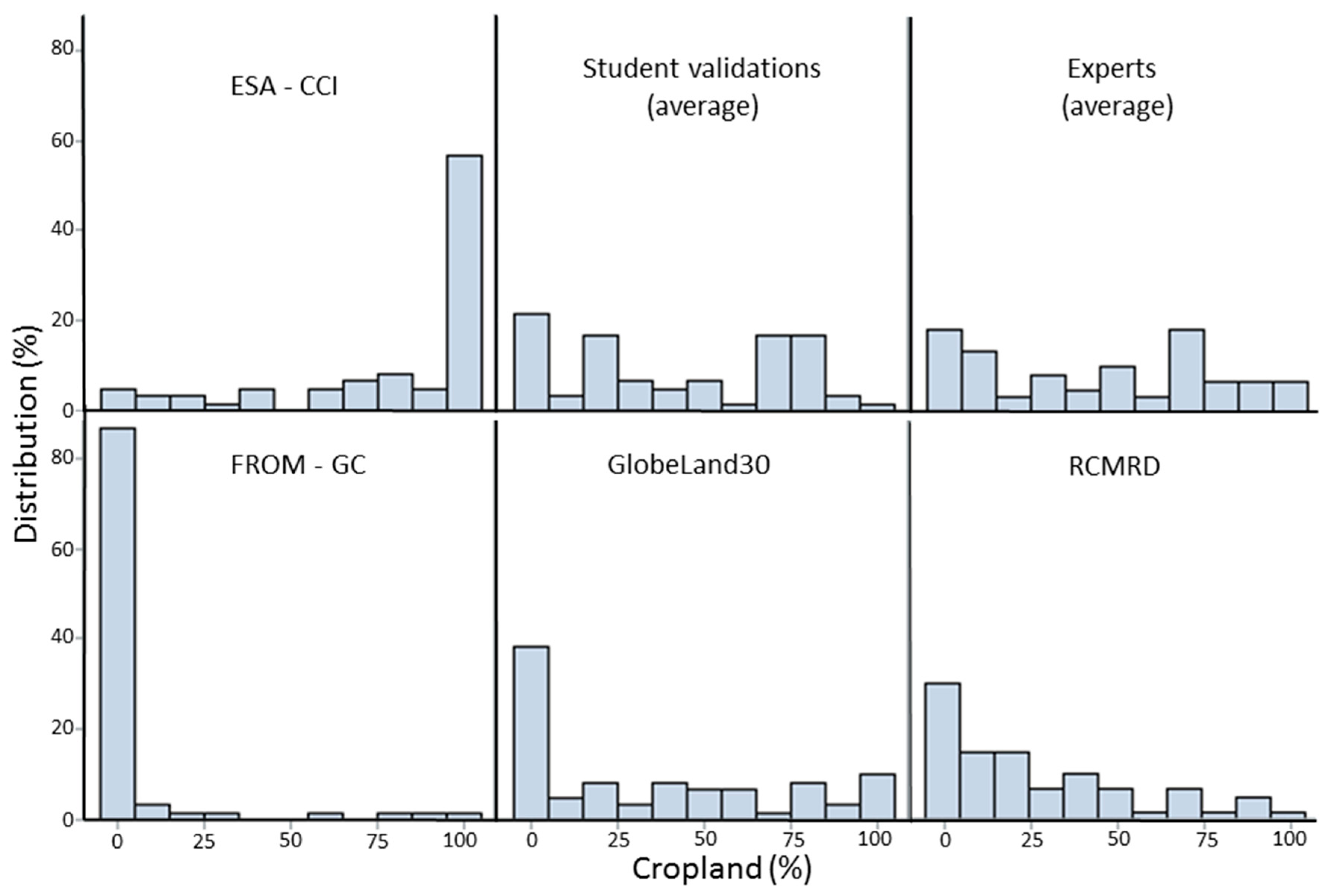
Figure 12.
Histograms of cropland percentage distribution for all data sets in the selected 60 locations where disagreement was highest including the expert evaluations.
Figure 12.
Histograms of cropland percentage distribution for all data sets in the selected 60 locations where disagreement was highest including the expert evaluations.
Figure 13.
Visual inspection of very high resolution imagery using Google Earth showing two example sites where ESA-CCI classified grassland/shrubland as cropland.
Figure 13.
Visual inspection of very high resolution imagery using Google Earth showing two example sites where ESA-CCI classified grassland/shrubland as cropland.
Table 1.
Data sets used in this study. * denotes frames containing Digital Globe very high resolution (VHR) imagery.
Table 1.
Data sets used in this study. * denotes frames containing Digital Globe very high resolution (VHR) imagery.
| Data Set | Reach | Resolution | Imagery Timespan |
|---|
| ESA-CCI | Global | 300 m | 2008–2012 (2010 baseline) |
| GlobeLand30 | Global | 30 m | 2008–2011 (2010 baseline) |
| FROM-GC | Global | 30 m | 2010 |
| RCMRD | Multi-national | 30 m | 2010 |
| Validation data from the students | National | 1 × 1 km frame * | 2005–2014 |
Table 2.
Descriptive statistics for the data collected through the Geo-Wiki interface for cropland and woody extent in percentage. Images with only one validation are excluded (N = 22,190).
Table 2.
Descriptive statistics for the data collected through the Geo-Wiki interface for cropland and woody extent in percentage. Images with only one validation are excluded (N = 22,190).
| Variable | Average Lowest | Average Mean | Average Highest |
|---|
| Cropland extent | 13.6 | 25.8 | 38.5 |
| Woody extent | 42.8 | 54.3 | 65.6 |
Table 3.
Cropland classes in each data set and their corresponding LCCS (Land Cover Classification System) notations.
Table 3.
Cropland classes in each data set and their corresponding LCCS (Land Cover Classification System) notations.
| Data Sets | Class | Definition | LCCS Label * | LCCS Code | LCCS Level |
|---|
| ESA-CCI | 10 | Cropland, rainfed | Rainfed shrub crops | 11494 | A2XXXXXXD1 |
| Rainfed tree crops | 11490 | A1XXXXXXD1 |
| Rainfed herbaceous crops | 11498 | A3XXXXXXD1 |
| 20 | Cropland, irrigated or post-flooding | Irrigated tree crops | 11491 | A1XXXXXXD3 |
| Irrigated shrub crops | 11495 | A2XXXXXXD3 |
| Irrigated herbaceous crops | 11500 | A3XXXXXXD3 |
| Post-flooding cultivation of herbaceous crops | 11499 | A3XXXXXXD2 |
| GlobeLand30 | 10 | Cultivated land: Lands used for agriculture, horticulture and gardens, including paddy fields, irrigated and dry farmland, vegetation and fruit gardens, etc. | Rainfed shrub crops | 11494 | A2XXXXXXD1 |
| Rainfed tree crops | 11490 | A1XXXXXXD1 |
| Rainfed herbaceous crops | 11498 | A3XXXXXXD1 |
| Irrigated tree crops | 11491 | A1XXXXXXD3 |
| Irrigated shrub crops | 11495 | A2XXXXXXD3 |
| Irrigated herbaceous crops | 11500 | A3XXXXXXD3 |
| Post-flooding cultivation of herbaceous crops | 11499 | A3XXXXXXD2 |
| FROM-GC | 11 | Crop-Rice | Irrigated herbaceous crops | 11500 | A3XXXXXXD3 |
| 12 | Crop-Greenhouse | NA † | NA | NA |
| 13 | Crop-Other | Herbaceous crop(s) | 10025 | A3 |
| Shrub crop(s) | 10013 | A2 |
| 94 | Bare-Cropland | Bare soil and/or other unconsolidated material(s) | 6005 | A5 |
| Herbaceous croplands | 10025 | A3 |
| RCMRD | 41 | Perennial Cropland | Rainfed shrub crops | 11494 | A2XXXXXXD1 |
| Rainfed tree crops | 11490 | A1XXXXXXD1 |
| Irrigated tree crops | 11491 | A1XXXXXXD3 |
| Irrigated shrub crops | 11495 | A2XXXXXXD3 |
| 42 | Annual Cropland | Rainfed herbaceous crops | 11498 | A3XXXXXXD1 |
| Irrigated herbaceous crops | 11500 | A3XXXXXXD3 |
| Post-flooding cultivation of herbaceous crops | 11499 | A3XXXXXXD2 |
| Validation data from the students | Scale: 1-2-3-4 | 1: No cropland, 2: Low cropland, 3: Medium cropland and 4: High cropland | Rainfed shrub crops | 11494 | A2XXXXXXD1 |
| Rainfed tree crops | 11490 | A1XXXXXXD1 |
| Rainfed herbaceous crops | 11498 | A3XXXXXXD1 |
| Irrigated tree crops | 11491 | A1XXXXXXD3 |
| Irrigated shrub crops | 11495 | A2XXXXXXD3 |
| Irrigated herbaceous crops | 11500 | A3XXXXXXD3 |
| Post-flooding cultivation of herbaceous crops | 11499 | A3XXXXXXD2 |
Table 4.
LCCS labels and their correspondence in each of the data sets used in the study. A check mark (✓) indicates correspondence with the LCCS label while an X (✘) denotes absence.
Table 4.
LCCS labels and their correspondence in each of the data sets used in the study. A check mark (✓) indicates correspondence with the LCCS label while an X (✘) denotes absence.
| LCCS-Label | Aggregated Class | ESA-CCI | GlobeLand30 | FROM-GC | RCMRD | Validation Data from the Students |
|---|
| Rainfed herbaceous crops | Herbaceous crops | ✓ | ✓ | ✓ | ✓ | ✓ |
| Irrigated herbaceous crops |
| Post-flooding cultivation of herbaceous crops |
| Herbaceous croplands |
| Rainfed shrub crops | Shrub Crops | ✓ | ✓ | ✓ | ✓ | ✓ |
| Irrigated shrub crops |
| Rainfed tree crops | Tree Crops | ✓ | ✓ | ✘ | ✓ | ✓ |
| Irrigated tree crops |
| Bare soil and/or other unconsolidated material(s) | | ✘ | ✘ | ✓ | ✘ | ✘ |
Table 5.
Confusion matrix showing number of images classified as no cropland (<10%), low (10–33.3%), medium (33.3–66.6%) and high (>66.6%) cropland by the students compared to the ESA-CCI data set across Tanzania (N = 22,190). A total of 3745 scenes have only one interpretation and are not compared. The classification uses the average values from each data set. Users and producers (weighted) accuracy with 95% confidence intervals are shown. The overall weighted accuracy is 0.46 ± 0.01.
| | Validation Data from the Students |
|---|
| No | Low | Mid | High | User Acc. |
|---|
| ESA-CCI | No | 5508 | 2046 | 972 | 325 | 0.62 ± 0.01 |
| Low | 986 | 552 | 405 | 187 | 0.26 ± 0.02 |
| Mid | 928 | 632 | 610 | 410 | 0.24 ± 0.02 |
| High | 1582 | 1573 | 2672 | 2802 | 0.32 ± 0.01 |
| Prod. Acc. | 0.69 ± 0.01 | 0.10 ± 0.01 | 0.14 ± 0.01 | 0.70 ± 0.02 | |
Table 6.
Confusion matrix showing number of images classified as no cropland (<10%), low (10–33.3%), medium (33.3–66.6%) and high (>66.6%) cropland by the students compared to the GlobeLand30 data set across Tanzania (N = 22,190). A total of 3745 scenes have only one interpretation and are not compared. The classification uses the average values from each data set. Users and producers (weighted) accuracy with 95% confidence intervals are shown. The overall weighted accuracy is 0.47 ± 0.01.
| | Validation Data from the Students |
|---|
| No | Low | Mid | High | User Acc. |
|---|
| GlobeLand30 | No | 8472 | 3839 | 2226 | 637 | 0.56 ± 0.01 |
| Low | 261 | 471 | 712 | 323 | 0.27 ± 0.02 |
| Mid | 138 | 263 | 770 | 629 | 0.43 ± 0.02 |
| High | 133 | 230 | 951 | 2135 | 0.62 ± 0.01 |
| Prod. Acc. | 0.68 ± 0.02 | 0.36 ± 0.02 | 0.34 ± 0.01 | 0.52 ± 0.02 | |
Table 7.
Confusion matrix showing number of images classified as no cropland (<10%), low (10–33.3%), medium (33.3–66.6%) and high (>66.6%) cropland by the students compared to the RCMRD data set across Tanzania (N = 22,190). A total of 3745 scenes have only one interpretation and are not compared. The classification uses the average values from each data set. Users and producers (weighted) accuracy with 95% confidence intervals are shown. The overall weighted accuracy is 0.43 ± 0.01.
| | Validation Data from the Students |
|---|
| No | Low | Mid | High | User Acc. |
|---|
| RCMRD | No | 7813 | 3541 | 2055 | 554 | 0.57 ± 0.01 |
| Low | 767 | 713 | 1008 | 648 | 0.23 ± 0.01 |
| Mid | 275 | 378 | 834 | 950 | 0.34 ± 0.02 |
| High | 149 | 171 | 762 | 1572 | 0.59 ± 0.02 |
| Prod. Acc. | 0.58 ± 0.01 | 0.33 ± 0.02 | 0.31 ± 0.01 | 0.48 ± 0.01 | |
Table 8.
Confusion matrix showing number of images classified as no cropland (<10%), low (10–33.3%), medium (33.3–66.6%) and high (>66.6%) cropland by the students compared to the FROM-GC data set across Tanzania (N = 22,190). A total of 3745 scenes have only one interpretation and are not compared. The classification uses the average values from each data set set. Users and producers (weighted) accuracy with 95% confidence intervals are shown. The overall weighted accuracy is 0.36 ± 0.01.
| | Validation Data from the Students |
|---|
| No | Low | Mid | High | User Acc. |
|---|
| FROM-GC | No | 8357 | 4187 | 3567 | 2437 | 0.45 ± 0.01 |
| Low | 332 | 284 | 366 | 368 | 0.21 ± 0.02 |
| Mid | 216 | 207 | 389 | 410 | 0.32 ± 0.03 |
| High | 99 | 125 | 337 | 509 | 0.47 ± 0.03 |
| Prod. Acc. | 0.47 ± 0.02 | 0.29 ± 0.02 | 0.29 ± 0.02 | 0.39 ± 0.02 | |
Table 9.
Confusion matrix showing number of images classified as no cropland (<10%), low (10–33.3%), medium (33.3–66.6%) and high (>66.6%) cropland by the students compared to the ESA-CCI data set for the Kilosa district (N = 12,373). A total of 2160 scenes have only one interpretation and are not compared. The classification uses the average values from each data set. Users and producers accuracy with 95% confidence intervals are shown. The overall accuracy is 0.42 ± 0.01.
| | Validation Data from the Students |
|---|
| No | Low | Mid | High | User Acc. |
|---|
| ESA-CCI | No | 2947 | 945 | 353 | 69 | 0.68 ± 0.01 |
| Low | 698 | 376 | 216 | 62 | 0.28 ± 0.02 |
| Mid | 655 | 426 | 369 | 181 | 0.23 ± 0.02 |
| High | 980 | 993 | 1606 | 1497 | 0.29 ± 0.01 |
| Prod. Acc. | 0.56 ± 0.01 | 0.14 ± 0.01 | 0.15 ± 0.01 | 0.83 ± 0.02 | |
Table 10.
Confusion matrix showing number of images classified as no cropland (<10%), low (10–33.3%), medium (33.3–66.6%) and high (>66.6%) cropland by the students compared to the GlobeLand30 data set for the Kilosa district (N = 12,373). A total of 2160 scenes have only one interpretation and are not compared. The classification uses the average values from each data set. Users and producers accuracy with 95% confidence intervals are shown. The overall accuracy is 0.54 ± 0.01.
| | Validation Data from the Students |
|---|
| No | Low | Mid | High | User Acc. |
|---|
| GlobeLand30 | No | 4956 | 2172 | 1222 | 350 | 0.57 ± 0.01 |
| Low | 168 | 285 | 411 | 140 | 0.28 ± 0.03 |
| Mid | 84 | 151 | 426 | 318 | 0.44 ± 0.03 |
| High | 72 | 132 | 485 | 1001 | 0.59 ± 0.02 |
| Prod. Acc. | 0.94 ± 0.01 | 0.10 ± 0.01 | 0.17 ± 0.01 | 0.55 ± 0.02 | |
Table 11.
Confusion matrix showing number of images classified as no cropland (<10%), low (10–33.3%), medium (33.3–66.6%) and high (>66.6%) cropland by the students compared to the RCMRD data set for the Kilosa district (N = 12,373). A total of 2160 scenes have only one interpretation and are not compared. Users and producers accuracy with 95% confidence intervals are shown. The classification uses the average values from each data set. The overall accuracy is 0.50 ± 0.01.
| | Validation Data from the Students |
|---|
| No | Low | Mid | High | User Acc. |
|---|
| RCMRD | No | 4569 | 2033 | 1169 | 277 | 0.57 ± 0.01 |
| Low | 476 | 413 | 558 | 325 | 0.23 ± 0.02 |
| Mid | 163 | 203 | 442 | 472 | 0.35 ± 0.03 |
| High | 72 | 91 | 375 | 735 | 0.58 ± 0.03 |
| Prod. Acc. | 0.87 ± 0.01 | 0.15 ± 0.01 | 0.17 ± 0.01 | 0.41 ± 0.02 | |
Table 12.
Confusion matrix showing number of images classified as no cropland (<10%), low (10–33.3%), medium (33.3–66.6%) and high (>66.6%) cropland by the students compared to the FROM-GC data set for the Kilosa district (N = 12,373). A total of 2160 scenes have only one interpretation and are not compared. Users and producers accuracy with 95% confidence intervals are shown. The classification uses the average values from each data set. The overall accuracy is 0.44 ± 0.01.
| | Validation Data from the Students |
|---|
| No | Low | Mid | High | User Acc. |
|---|
| FROM-GC | No | 5215 | 2655 | 2338 | 1577 | 0.44 ± 0.01 |
| Low | 35 | 52 | 92 | 93 | 0.19 ± 0.05 |
| Mid | 25 | 17 | 77 | 78 | 0.39 ± 0.07 |
| High | 5 | 16 | 37 | 61 | 0.51 ± 0.09 |
| Prod. Acc. | 0.99 ± 0.01 | 0.02 ± 0.01 | 0.03 ± 0.01 | 0.03 ± 0.01 | |
Table 13.
Confusion matrix showing the number of images classified as no cropland, low, medium, and high cropland by the students compared to the expert classification on 60 locations where disagreement between the products was high. Users and producers accuracy with 95% confidence intervals are shown. The classification uses the average values from each data set. The overall accuracy is 0.60 ± 012.
| | Expert Evaluations |
|---|
| No | Low | Mid | High | User Acc. |
|---|
| Validation data from the students | No | 11 | 1 | 1 | 1 | 0.79 ± 0.22 |
| Low | 4 | 3 | 4 | 1 | 0.40 ± 0.26 |
| Mid | 0 | 0 | 6 | 5 | 0.44 ± 0.31 |
| High | 0 | 3 | 4 | 16 | 0.69 ± 0.19 |
| Prod. Acc. | 0.73 ± 0.17 | 0.43 ± 0.34 | 0.40 ± 0.20 | 0.70 ± 0.15 | |


 ,
, 


