Influence of Droughts on Mid-Tropospheric CO2
by
 ,
,
Xun Jiang
1,*, 
Angela Kao
1,
Abigail Corbett
1,
Edward Olsen
2,
Thomas Pagano
2,
Albert Zhai
3,4,
Sally Newman
3,
Liming Li
5 and
Yuk Yung
3 1
Department of Earth & Atmospheric Sciences, University of Houston, Houston, TX 77004, USA
2
Science Division, Jet Propulsion Laboratory, California Institute of Technology, 1200 E California Blvd, Pasadena, CA 91125, USA
3
Division of Geological and Planetary Sciences, California Institute of Technology, 1200 E California Blvd, Pasadena, CA 91125, USA
4
La Cañada High School, La Cañada Flintridge, Los Angeles, CA 91011, USA
5
Department of Physics, University of Houston, Houston, TX 77004, USA
*
Author to whom correspondence should be addressed.
Remote Sens. 2017, 9(8), 852; https://doi.org/10.3390/rs9080852
Submission received: 16 June 2017
/
Revised: 13 August 2017
/
Accepted: 15 August 2017
/
Published: 17 August 2017
(This article belongs to the Special Issue Remote Sensing of Greenhouse Gases)
Abstract
:Using CO2 data from the Atmospheric Infrared Sounder (AIRS), it is found for the first time that the mid-tropospheric CO2 concentration is ~1 part per million by volume higher during dry years than wet years over the southwestern USA from June to September. The mid-tropospheric CO2 differences between dry and wet years are related to circulation and CO2 surface fluxes. During drought conditions, vertical pressure velocity from NCEP2 suggests that there is more rising air over most regions, which can help bring high surface concentrations of CO2 to the mid-troposphere. In addition to the circulation, there is more CO2 emitted from the biosphere to the atmosphere during droughts in some regions, which can contribute to higher concentrations of CO2 in the atmosphere. Results obtained from this study demonstrate the significant impact of droughts on atmospheric CO2 and therefore on a feedback cycle contributing to greenhouse gas warming. It can also help us better understand atmospheric CO2, which plays a critical role in our climate system.
1. Introduction
In addition to the trend [1,2,3] and the annual cycle [4,5,6,7,8,9], atmospheric CO2 also demonstrates a lot of intra-seasonal [10,11] and inter-annual variability [12,13,14,15]. During the pre-satellite era, CO2 analyses mainly utilized in-situ CO2 measurements to investigate CO2 variability, which is limited in space. In recent years, CO2 retrievals from different satellites [16,17,18,19,20,21] provide CO2 concentrations over the global domain, which can be used to explore CO2 variability at different locations. Utilizing the mid-tropospheric CO2 from Atmospheric Infrared Sounder (AIRS), it has been found that large-scale processes (e.g., Madden-Julian Oscillation, El Niño-Southern Oscillation, South-Atlantic Walker circulation, and Northern Annular Mode) can modulate CO2 concentrations in the middle troposphere [10,14,22].
In addition to the influences from large-scale processes, surface CO2 emissions can also change atmospheric CO2 concentrations in the middle troposphere [23]. Pagano et al. [23] investigated the correlation between mid-tropospheric CO2 and gross primary production (GPP) from the biosphere in July at 40°N–50°N and found a correlation coefficient of −0.8 between mid-tropospheric CO2 and the GPP. Large GPP means more photosynthesis, thus more CO2 uptake from biosphere and less CO2 in the atmosphere.
Using CO2 data over Mauna Loa, Buermann et al. [8] found that the decline in the CO2 seasonal cycle amplitudes since the early 1990s is related to reductions in the carbon sequestration as responses to severe droughts and changes in the atmospheric circulation. Norman et al. [24] measured soil surface CO2 fluxes at three sites and found that the soil surface CO2 fluxes are sensitive to the drought and temperature. By analyzing soil surface CO2 flux over grassland, Laporte et al. [25] have found that decreasing rain events will lead to less soil surface CO2 flux and reduced plant growth. Zhou et al. [26] found that the soil surface CO2 fluxes will increase when temperature and precipitation increase. Pereira et al. [27] analyzed the impact of droughts on net ecosystem carbon exchange in three Mediterranean ecosystems and found that droughts will influence gross primary production more than the ecosystem respiration. Parton et al. [28] analyzed net ecosystem production on the short grass steppe vegetation and found that net carbon uptake is reduced during low precipitation events. These pervious analyses [8,24,25,26,27,28] mainly focus on measurements over a small area. Global distributed CO2 data from AIRS offer a unique opportunity to explore the impact of droughts on atmospheric CO2 over large spatial domain.
In recent years, the drought has become a severe problem over the southwestern USA. The recent drought in California is the most severe in the past 1200 years [29]. However, investigations of the relationship between the drought events and the concentration of CO2 over the southwestern USA are lacking. The relatively long-term CO2 retrievals from AIRS provide a unique opportunity to examine such a relationship. In this paper, we will combine satellite CO2, vertical pressure velocity, and CO2 surface emissions to investigate the impact of droughts on CO2 concentrations in the mid-troposphere over southwest USA.
2. Data
Tropical Rainfall Measuring Mission (TRMM) precipitation is employed to identify dry and wet years in this paper. TRMM precipitation data (Version 7 3A12) are available from 1998 to the present covering 50°S–50°N. The spatial resolution of TRMM precipitation is 0.25° in latitude and 0.25° in longitude. TRMM calibrated precipitation data include observations from several different instruments (TMI, AMSR-E, SSM/I, and AMSU-B) [30].
AIRS Version 5 mid-tropospheric CO2 mixing ratios [16,22,31] are used in this paper to explore the influence of droughts on atmospheric CO2. The Vanishing Partial Derivative (VPD) Method [16,31,32] is used to retrieve AIRS mid-tropospheric CO2 data, which has a maximum sensitivity at 500–300 hPa. The spatial resolution of AIRS CO2 retrieval is 2° in latitude and 2.5° in longitude covering 60°S to 90°N. AIRS mid-tropospheric CO2 data are available from September 2002 to December 2013 and can be downloaded at http://disc.sci.gsfc.nasa.gov/AIRS/data-holdings/by-data-product-v5/AIRX3C2M [32]. A comparison between AIRS mid-tropospheric CO2 and convolved INTEX-NA aircraft CO2 reveals a difference of 0.15 ppm with a standard deviation of 0.71 ppm [16,31,32]. AIRS mid-tropospheric CO2 has also been compared with CONTRAIL aircraft CO2 and there is a bias of 0.1 ppm with a standard deviation of 1.8 ppm [16,31,32].
CO2 surface fluxes from the biosphere and biomass burning are used to explore CO2 surface emissions during dry and wet years. The exchange of CO2 between biosphere and atmosphere from the Carnegie-Ames Stanford Approach (CASA) biogeochemical model [33,34,35,36,37,38] is utilized to explore the biosphere–atmosphere interaction during dry and wet years. The CASA model uses satellite data and a mechanistic plant and soil carbon model to simulate the carbon from the terrestrial ecosystem [33,34,35]. Influences of the Normalized Difference Vegetation Index (NDVI), weather, and fire on biosphere are considered in the CASA model [36,37,38]. Satellite NDVI data are used to parameterize net primary production in the CASA model [39], which calculates the exchange of CO2 between the atmosphere and biosphere at different time steps and different spatial resolution. Net Ecosystem CO2 Exchange (NEE), Gross Primary Production (GPP), and ecosystem respiration from the CASA biogeochemical model will be used to explore the influence of droughts on CO2 fluxes from the biosphere. NEE represents the net exchange of CO2 between the biosphere and the atmosphere, which is calculated as the difference between ecosystem respiration and GPP. Ecosystem respiration represents the autotrophic and heterotrophic respiration from the biosphere. GPP is related to the carbon uptake by plants during the photosynthesis. CO2 biomass burning emissions are from Global Fire Emissions Database Version 4.1 (GFEDv4.1) [40]. CO2 emissions from biosphere and biomass burning are available at 0.25 × 0.25° (latitude by longitude). These data are monthly means from 1997 through 2013.
Vertical pressure velocity data at 500 hPa from the National Centers for Environmental Prediction 2 (NCEP2) Reanalysis data [41] are used in this paper to explore the influence of circulation on CO2 during dry and wet years. Vertical pressure velocity is defined as the rate of change of pressure (P) with time (t) (dP/dt). The spatial resolution of vertical pressure velocity data is 2.5° in latitude and 2.5° in longitude. Monthly mean data are available from 1979 to present.
3. Results
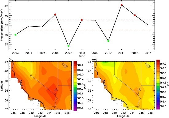
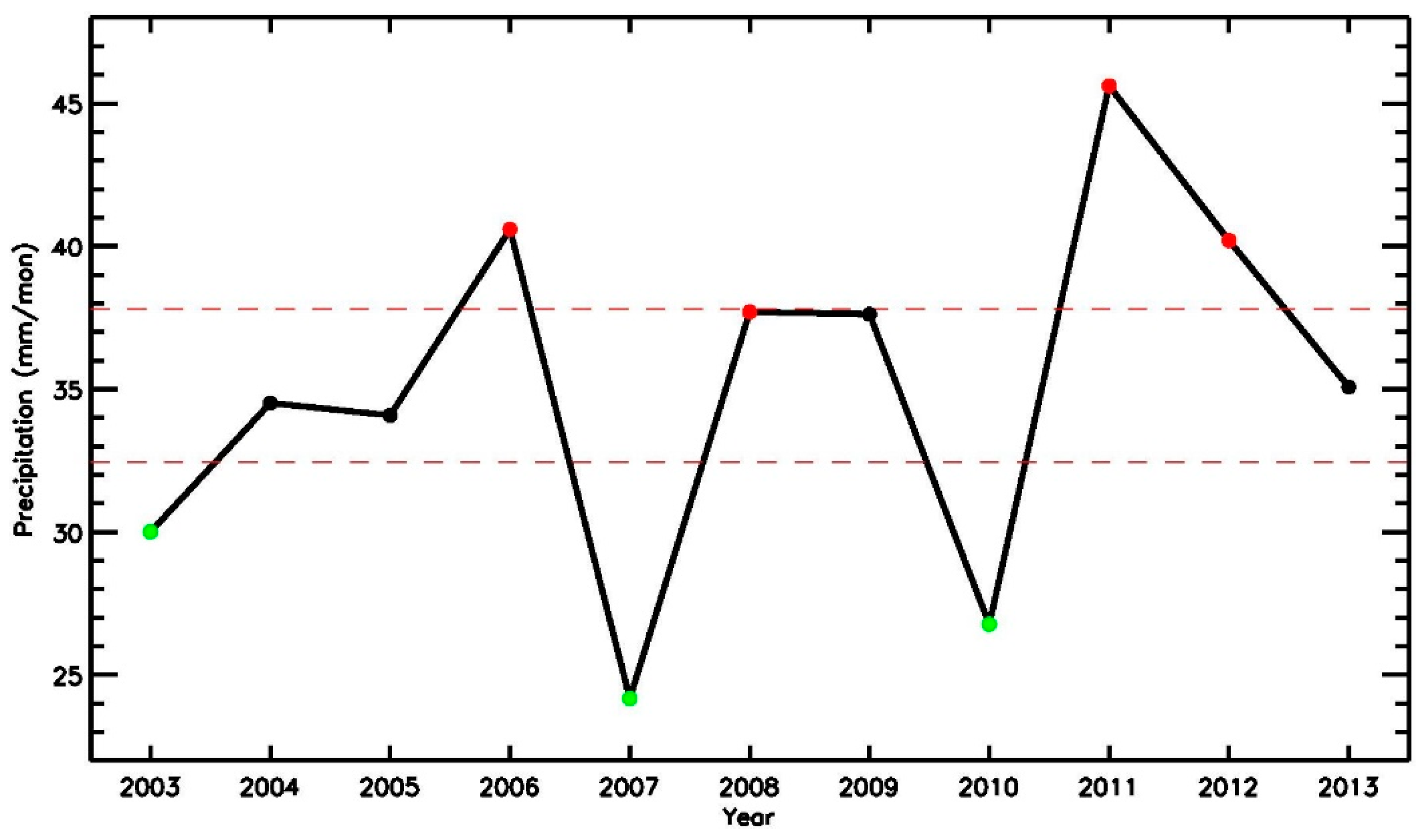
To identify wet and dry years, we calculate averaged TRMM precipitation over the southwestern USA (32°N–42°N, 235°E–249°E) from June through September (JJAS) in 2003–2013, as well as the mean value and the standard deviation of these data. When the precipitation is 0.5 times standard deviation above (below) the mean value (35.1 mm), it is classified as a wet (dry) year. Red dashed lines in Figure 1 represent mean precipitation ±0.5 times standard deviation of TRMM precipitation. As shown by red dots in Figure 1, 2006, 2008, 2011, and 2012 are wet years. Dry years (2003, 2007, and 2010) are shown by green dots in Figure 1.
To investigate the influence of droughts on AIRS mid-tropospheric CO2, we first remove the linear trend [42] from the AIRS mid-tropospheric CO2 data. We then calculate mean values of AIRS detrended CO2 for dry years (JJAS of 2003, 2007, and 2010) and wet years (JJAS of 2006, 2008, 2011, and 2012) separately. Figure 2a,b demonstrate spatial patterns of the detrended AIRS mid-tropospheric CO2 for dry years and wet years, respectively. The difference of the detrended AIRS mid-tropospheric CO2 between dry years (JJAS of 2003, 2007, and 2010) and wet years (JJAS of 2006, 2008, 2011, and 2012) is shown in Figure 2c. There is more CO2 over the southwestern USA during dry years than wet years. The CO2 difference between dry and wet years is ~1 ppm. There are ~4000 AIRS CO2 retrievals in each grid box for dry and wet months. Since the error for an individual CO2 retrieval follows a Gaussian distribution and is random [31], the CO2 error in each grid box is equal to the CO2 standard error (~1–2 ppm) divided by the square root of number of data [22]. As a result, the error for the CO2 is less than 0.1 ppm, which is significantly less than the 1 ppm difference between dry and wet years shown in Figure 2c.
A bootstrap method is used to calculate the statistical significance of CO2 differences between dry years and wet years [43,44]. The bootstrap method can be used for any distribution function of the data [43]. We generate 3000 bootstrap samples for the data in each grid. For each bootstrap sample, we repeat random re-sampling of the data, which will be further utilized to estimate the confidence interval at each grid. The CO2 differences statistically significant at the 5% significance level and 1% significance level are plotted as light green and dark green areas in Figure 2d. Results are considered to be statistically significant when the significance level is 5% or less, which corresponds to two standard deviations [42]. As shown in Figure 2d, the CO2 difference is within the 5% significance level in all regions.
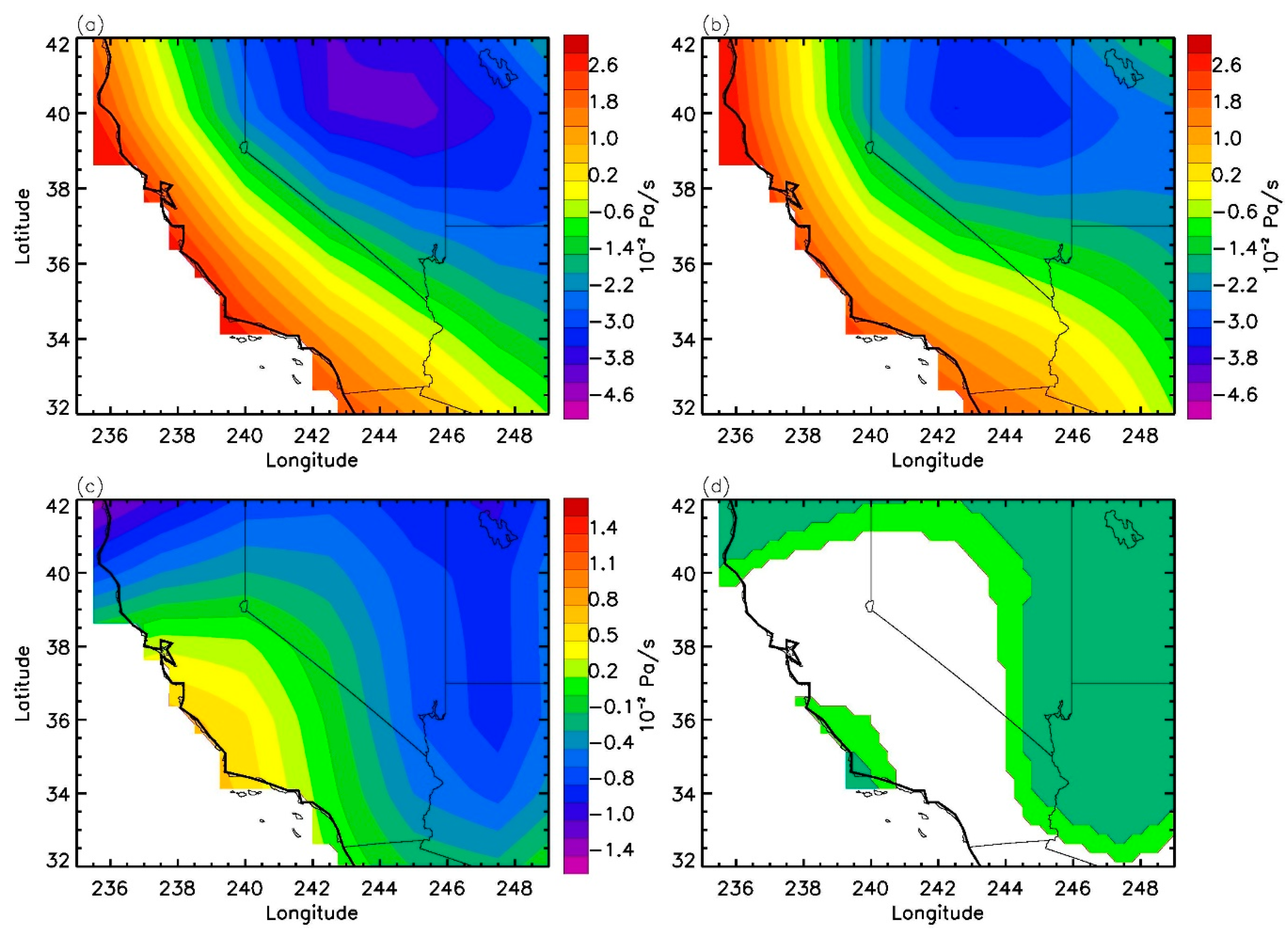
To explore possible mechanisms for high CO2 concentrations during dry years, we investigate the 500 hPa vertical pressure velocity and CO2 surface emissions during dry and wet years. Vertical pressure velocity during dry years and wet years are shown in Figure 3a,b, respectively. Negative values of vertical pressure velocity represent rising air, while positive values of vertical pressure velocity represent sinking air. As shown in Figure 3a,b, there is rising air over most regions for both dry years and wet years. The difference of 500 hPa vertical pressure velocity between dry years and wet years is shown in Figure 3c. There is stronger rising motion in dry years than in wet years over northern California, Nevada, Utah, and Arizona. The stronger rising motion in the dry years can bring more CO2 from surface to the mid-troposphere, which contributes to the high CO2 concentrations in the mid-troposphere during dry years. The surface temperature is higher over inland regions during dry years than wet years, resulting in an unstable environment, which will move air from the surface to the mid-troposphere. Rising air can further bring high concentration CO2 from the surface to the mid-troposphere, which leads to positive CO2 anomalies during dry conditions.
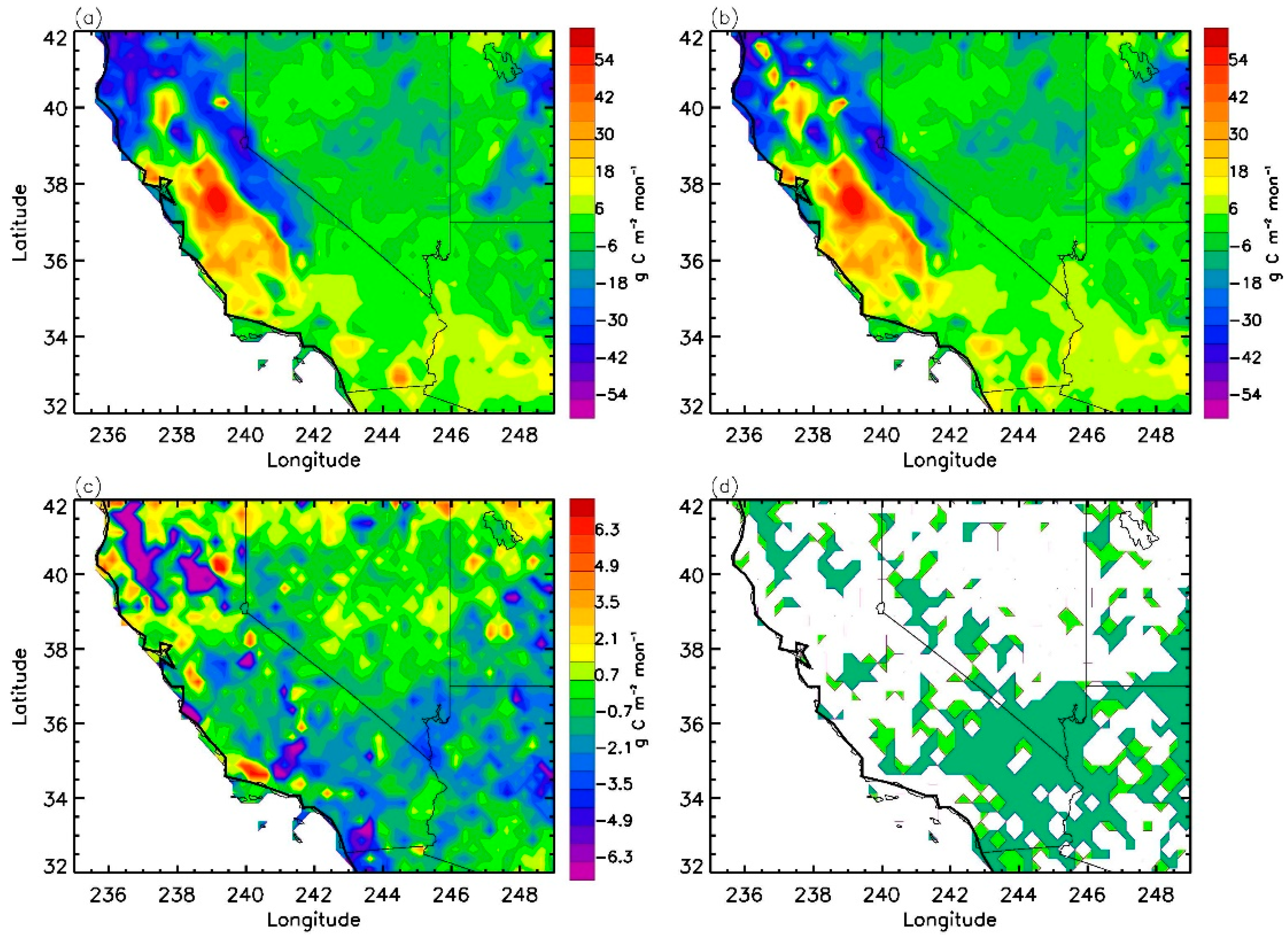
In addition to the vertical pressure velocity, we also explore the CO2 surface emissions to see if CO2 surface emissions can influence mid-tropospheric CO2 concentrations during drought conditions. The mean values of Net Ecosystem Exchange (NEE) during dry years and wet years are shown in Figure 4a,b. NEE represents the net exchange between the biosphere and the atmosphere. Positive NEE means that CO2 is released from biosphere to atmosphere, while negative NEE suggests that CO2 is removed from the atmosphere by vegetative uptake. As shown in Figure 4a,b, NEE is positive over southern California and Arizona and negative over northern California and part of Utah. NEE differences between dry years and wet years are shown in Figure 4c. As shown in Figure 4c, there are positive NEE anomalies over most regions of Nevada, Utah, and part of California and Arizona during dry years, which mean more CO2 is released to the atmosphere from biosphere during dry years in these regions. The increased CO2 released from the biosphere can contribute to high CO2 concentrations during dry years. There are also some negative NEE anomalies over California and Arizona during dry years.
Since NEE is related to photosynthesis and respiration from the biosphere, we explore Gross Primary Production (GPP) and ecosystem respiration in Figures S1 and S2 in the Supplementary Materials. GPP represents photosynthesis by the biosphere. The difference in GPP between dry years and wet years is shown in Figure S1c. Negative GPP anomalies are seen over Nevada and California in Figure S1c, which suggests that there is less photosynthesis by the biosphere during dry years. Less photosynthesis means less CO2 uptake from biosphere. Thus, there will be more CO2 remaining in the atmosphere during dry years over Nevada and California. There are also positive anomalies of GPP over Arizona and Utah, which means more CO2 is removed from the atmosphere over these regions during the dry years, which will be partly canceled by the positive anomalies of ecosystem respiration in the same regions (Figure S2c). As shown in Figure S2c, the difference in respiration is positive over Nevada, Utah, Arizona, and some areas in California, which suggests more CO2 is released to the atmosphere due to respiration during dry years over these regions. These increased biospheric emissions will contribute to the positive CO2 anomaly in the atmosphere. There are also some negative anomalies of respiration over California, which corresponds to lower CO2 emissions to the atmosphere due to the respiration.
In addition to the net exchange between biosphere and atmosphere, we also explore CO2 biomass burning during dry and wet years (Figure S3c). The difference in CO2 from biomass burning between dry and wet years is a little noisy. As shown in Figure S3c, there are positive CO2 anomalies from biomass burning over some areas. However, there are also some negative CO2 anomalies, which might be related to different locations of biomass burning during different years.
Finally, we explore the influence of droughts on fossil fuel CO2 emissions. We analyze monthly mean fossil fuel CO2 emissions from the Carbon Dioxide Information Analysis Center (CDIAC) [45]. As shown in Figure S4c, the difference of fossil fuel CO2 emissions is small between dry months and wet months. Although there are very weak CO2 anomalies over southern California and southern Arizona, the anomalies are not statistically significant. This might be because the fossil fuel CO2 emissions are anthropogenic sources of atmospheric CO2, so the influence of droughts on fossil fuel CO2 emissions is small. Human activities continue despite the occurrence of droughts.
4. Discussion
In this paper, we explore the influences of droughts on CO2 and discuss possible sources (e.g., circulation, NEE, biomass burning, and fossil fuel emissions) for the CO2 anomalies in the atmosphere. It should be mentioned that the NEE from CASA model also has some limitations. For example, the CASA model used in this paper does not include CO2 and nitrogen fertilization, which might influence the NEE results. Yang et al. [46] utilized TCCON column CO2 and aircraft profile CO2 to estimate NEE and found that the CASA model underestimates the NEE by 25%. In another study, Jiang et al. [47] found that NEE from the CASA model is underestimated in the mid-latitudes. One way to improve the model is to use more observations. We can use an inverse model (such as GEOS-Chem adjoint model) to identify possible weakness in the CO2 surface fluxes. Observation data, such as AIRS CO2, can be used to better understand/constrain the net ecosystem exchange from the CASA model by the inverse modeling in the future.
In addition to the factors discussed above, other factors can also affect the CO2 fluxes during droughts. In both urban and farm areas, there is more irrigation to help crops and landscapes to survive during droughts, which will lead to a small difference of CO2 fluxes from biosphere and soil during dry and wet months. During dry months, surface temperature is higher than during wet months. The high-temperature anomalies result in warm soil, which leads to increased CO2 emissions due to decomposition in the soil [48]. Moisture can contribute even more to the positive CO2 anomaly in the atmosphere. Meanwhile, low soil moisture during droughts will limit plant growth, which can also influence the CO2 flux from the biosphere.
In this paper, we focus on the influence of droughts on CO2 over the southwestern USA, since drought has been a severe problem over this region in recent years. Precipitation has different behaviors over different regions; for example, precipitation increases in some areas while decreases in other areas [49,50,51]. We will explore the impacts of droughts on CO2 in other regions in the future.
5. Conclusions
CO2 and precipitation play critical roles in global warming and the hydrological cycle, respectively. The long-term CO2 retrievals from the AIRS aboard the Aqua satellite and the precipitation measurements from the TRMM provide a great opportunity to explore the interaction between CO2 and precipitation. Our analyses based on new observations suggest that the mid-tropospheric CO2 concentrations are higher during dry years than wet years over the southwest USA. Results in this paper provide an insight on how droughts can influence CO2 concentrations in the mid-troposphere. Mid-tropospheric CO2 concentrations are ~1 ppm higher during dry years than wet years.
We further use reanalysis meteorology datasets to explore the physics behind the relationship between drought and CO2. As shown by NCEP2 vertical pressure velocity data, there is stronger rising motion over the southwestern USA during drought conditions, which can bring high CO2 concentrations from the surface to the mid-troposphere and help increase the CO2 concentration in the mid-troposphere during dry years. CO2 surface fluxes (NEE, GPP, respiration, and biomass burning) are used to explore the impact of droughts on the CO2 surface fluxes. The signals in the CO2 surface fluxes are a little noisy. During dry years, there is less CO2 uptake from the biosphere due to decreased photosynthesis in some regions (e.g. northern California and Nevada). As a result, more CO2 will remain in the atmosphere. There are also positive anomalies of CO2 emissions associated with respiration over Arizona, Utah, and Nevada. Positive anomalies of CO2 from biomass burning are also seen in some regions. These results suggest that vertical velocity and biospheric activities can contribute to the positive CO2 anomaly during droughts.
Results obtained from this study suggest that droughts over the southwestern USA lead to more CO2 in the mid-tropospheric atmosphere during the dry years. Our analyses also suggest that the atmospheric dynamics (e.g., vertical motion) affects the concentration of CO2 in the mid-troposphere. Finally, the relationship between the CO2 concentrations and the surface biologic activities explored in this study will help us better understand the interaction between biosphere and atmosphere. The frequencies of extreme weather events (such as droughts and floods) have increased over the last decade, consistent with a warmer and wetter atmosphere driven by radiative imbalance from greenhouse gas warming [52]. This paper reveals that droughts can in turn change the CO2 concentrations in the atmosphere.
Results from this paper can help us better understand CO2 and precipitation, two important components of the climate system. Observational studies provide constraints that must be incorporated into models, and hence this study will benefit the validation and development of models. Analyses in this study are also applicable for other regions of the world. This study helps us better understand Earth’s climate system and provide a quantitatively analysis of the impact of droughts on trace gases.
Supplementary Materials
The following are available online at www.mdpi.com/2072-4292/9/8/852/s1, Figure S1: (a) The mean value of Gross Primary Production (GPP) in dry years (JJAS of 2003, 2007, and 2010), (b) The mean value of GPP in wet years (JJAS of 2006, 2008, 2011, and 2012), (c) GPP differences between the dry and wet years. (d) GPP differences within 10% significance level are highlighted in green. Units for GPP are g C m-2 mon-1 in (a)-(c), Figure S2: (a) The mean value of Ecosystem Respiration (Re) in dry years (JJAS of 2003, 2007, and 2010), (b) The mean value of Re in wet years (JJAS of 2006, 2008, 2011, and 2012), (c) Re differences between the dry and wet years. (d) Re differences within 10% significance level are highlighted in green. Units for Re are g C m-2 mon-1 in (a)-(c), Figure S3: (a) The mean value of biomass burning in dry years (JJAS of 2003, 2007, and 2010), (b) The mean value of biomass burning in wet years (JJAS of 2006, 2008, 2011, and 2012), (c) Biomass burning differences between the dry and wet years, (d) Biomass burning differences within 10% significance level are highlighted in green. Units for biomass burning are g C m-2 mon-1 in (a)-(c).
Acknowledgments
We thank three anonymous referees and editor for their time and helpful comments. X.J. and Y.Y. were supported by NASA grants NNX13AC04G and NNX13AK34G. E.O. and T.P. conducted the work at the Jet Propulsion Laboratory, under contract with NASA. L.L. was supported by NASA ROSES Cassini Data Analysis and NASA grant NNH15ZDA001N-PDART.
Author Contributions
X.J. and A.K. conducted the analysis and wrote the manuscript. A.C., E.O., T.P., A.Z., S.N., L.L., and Y.Y. contributed to the result discussions and manuscript preparation.
Conflicts of Interest
The authors declare no competing financial interest.
References
- Keeling, C.D.; Whorf, T.P.; Wahlen, M.; Vanderplicht, J. Interannual extremes in the rate of rise of atmospheric carbon dioxide since 1980. Nature 1995, 375, 666–670. [Google Scholar] [CrossRef]
- Sarmiento, J.L.; Wofsy, S. A U.S. Carbon Cycle Science Plan. Available online: https://pdfs.semanticscholar.org/7c66/6a32b540b0a1fdf6497b5b4aae261055a802.pdf (accessed on August 2011).
- Tans, P.; Keeling, R. Trends in Atmospheric Carbon Dioxide. Available online: http://www.esrl.noaa.gov/gmd/ccgg/trends/ (accessed on 16 August 2017).
- Pearman, G.I.; Hyson, P. The annual variation of atmospheric CO2 concentration observed in the northern hemisphere. J. Geophys. Res. 1981, 86, 9839–9843. [Google Scholar] [CrossRef]
- Cleveland, M.S.; Freeny, A.E.; Graedel, T.E. The seasonal component of atmospheric CO2: Information from new approaches to the decomposition of seasonal time series. J. Geophys. Res. 1983, 88, 10934–10946. [Google Scholar] [CrossRef]
- Bacastow, R.B.; Keeling, C.D.; Whorf, T.P. Seasonal amplitude increase in atmospheric CO2 concentration at Mauna Loa, Hawaii, 1959–1982. J. Geophys. Res. 1985, 90, 10529–10540. [Google Scholar] [CrossRef]
- Keeling, C.D.; Chin, J.F.S.; Whorf, T.P. Increased activity of northern hemispheric vegetation inferred from atmospheric CO2 measurements. Nature 1996, 382, 146–149. [Google Scholar] [CrossRef]
- Buermann, W.; Lintner, B.R.; Koven, C.D.; Angert, A.; Pinzon, J.E.; Tucker, C.J.; Fung, I.Y. The changing carbon cycle at the Mauna Loa Observatory. Proc. Nat. Acad. Sci. USA 2007, 104, 4249–4254. [Google Scholar] [CrossRef] [PubMed]
- Jiang, X.; Crisp, D.; Olsen, E.T.; Kulawik, S.S.; Miller, C.E.; Pagano, T.S.; Liang, M.; Yung, Y.L. CO2 annual and semi-annual cycles from multiple satellite retrievals and models. Earth Space Sci. 2016. [Google Scholar] [CrossRef]
- Li, K.F.; Tian, B.; Waliser, D.E.; Yung, Y.L. Tropical mid-tropospheric CO2 variability driven by the Madden-Julian Oscillation. Proc. Nat. Acad. Sci. USA 2010, 107, 19171–19175. [Google Scholar] [CrossRef] [PubMed]
- Jiang, X.; Li, Q.; Chahine, M.T.; Yung, Y.L. CO2 semi-annual oscillation in the middle troposphere and at the surface. Glob. Biogeochem. Cycles 2012, 26. [Google Scholar] [CrossRef]
- Jones, C.D.; Collins, M.; Cox, P.M.; Spall, S.A. The carbon cycle response to ENSO: A coupled climate-carbon cycle model study. J. Clim. 2001, 14, 4113–4129. [Google Scholar] [CrossRef]
- Nevison, C.D.; Mahowald, N.M.; Doney, S.C.; Lima, I.D.; van der Werf, G.R.; Randerson, J.T.; Baker, D.F.; Kasibhatla, P.; McKinley, G.A. Contribution of ocean, fossil fuel, land biosphere, and biomass burning carbon fluxes to seasonal and interannual variability in atmospheric CO2. J. Geophys. Res. 2008, 113. [Google Scholar] [CrossRef]
- Jiang, X.; Chahine, M.T.; Olsen, E.T.; Chen, L.; Yung, Y.L. Interannual Variability of Mid-tropospheric CO2 from Atmospheric Infrared Sounder. Geophys. Res. Lett. 2010, 37. [Google Scholar] [CrossRef]
- Jiang, X.; Wang, J.; Olsen, E.T.; Liang, M.; Pagano, T.S.; Chen, L.; Licata, S.J.; Yung, Y.L. Influence of El Nino on mid-tropospheric CO2 from Atmospheric Infrared Sounder and Model. J. Atmos. Sci. 2013, 70, 223–230. [Google Scholar] [CrossRef]
- Chahine, M.; Chen, L.; Dimotakis, P.; Jiang, X.; Li, Q.; Olsen, E.T.; Pagano, T.; Randerson, J.; Yung, Y.L. Satellite remote sounding of mid-tropospheric CO2. Geophys. Res. Lett. 2008, 35. [Google Scholar] [CrossRef]
- Crevoisier, C.; Chédin, A.; Matsueda, H.; Machida, T.; Armante, R.; Scott, N.A. First year of upper tropospheric integrated content of CO2 from IASI hyperspectral infrared observations. Atmos. Chem. Phys. 2009, 9, 4797–4810. [Google Scholar] [CrossRef]
- Kulawik, S.S.; Jones, D.B.A.; Nassar, R.; Irion, F.W.; Worden, J.R.; Bowman, K.W.; Machida, T.; Matsueda, H.; Sawa, Y.; Biraud, S.C.; et al. Characterization of Tropospheric Emission Spectrometer (TES) CO2 for carbon cycle science. Atmos. Chem. Phys. 2010, 10, 5601–5623. [Google Scholar] [CrossRef]
- Boesch, H.; Baker, D.; Connor, B.; Crisp, D.; Miller, C. Global characterization of CO2 column retrievals from shortwave-infrared satellite observations of the Orbiting Carbon Observatory-2 Mission. Remote Sens. 2011, 3, 270–304. [Google Scholar] [CrossRef]
- Kulawik, S.S.; O’Dell, C.; Payne, V.H.; Kuai, L.; Worden, H.M.; Biraud, S.C.; Sweeney, C.; Stephens, B.; Iraci, L.T.; Yates, E.L.; Tanaka, T. Lower-tropospheric CO2 from near-infrared ACOS-GOSAT observations. Atmos. Chem. Phys. 2017, 17, 5407–5438. [Google Scholar] [CrossRef]
- Crisp, D.; Pollock, H.R.; Rosenberg, R.; Chapsky, L.; Lee, R.A.M.; Oyafuso, F.A.; Frankenberg, C.; O’Dell, C.W.; Bruegge, C.J.; Doran, G.B.; et al. The on-orbit performance of the Orbiting Carbon Observatory-2 (OCO-2) instrument and its radiometrically calibrated products. Atmos. Meas. Tech. 2017, 10, 59–81. [Google Scholar] [CrossRef]
- Jiang, X.; Olsen, E.; Pagano, T.; Su, H.; Yung, Y.L. Modulation of midtropospheric CO2 by the South Atlantic Walker Circulation. J. Atmos. Sci. 2015, 72, 2241–2247. [Google Scholar] [CrossRef]
- Pagano, T.S.; Olsen, E.T.; Nguyen, H.; Ruzmaikin, A.; Jiang, X.; Perkins, L. Global variability of midtropospheric carbon dioxide as measured by the Atmospheric Infrared Sounder. J. Appl. Remote Sens. 2014, 8. [Google Scholar] [CrossRef]
- Norman, J.M.; Garcia, R.; Verma, S.B. Soil surface CO2 fluxes and carbon budget of a grassland. J. Geophys. Res. 1992. [Google Scholar] [CrossRef]
- Laporte, M.F.; Duchesne, L.C.; Wetzel, S. Effect of rainfall patterns on soil surface CO2 efflux, soil moisture, soil temperature and plant growth in a grassland ecosystem of northern Ontario, Canada: Implications for climate change. BMC Ecol. 2002. [Google Scholar] [CrossRef]
- Zhou, X.; Sherry, R.A.; An, Y.; Wallace, L.L.; Luo, Y. Main and interactive effects of warming, clipping, and doubled precipitation on soil CO2 efflux in a grassland ecosystem. Glob. Biogeochem. Cycle 2006. [Google Scholar] [CrossRef]
- Pereira, J.S.; Mateus, J.A.; Aires, L.M.; Pita, G.; Pio, C.; David, J.S.; Andrade, V.; Banza, J.; David, T.S.; Paco, T.A.; Rodrigues, A. Net ecosystem carbon exchange in three constrasting Mediterranean ecosystems: The effect of drought. Biogeosciences 2007, 4, 791–802. [Google Scholar] [CrossRef]
- Parton, W.; Morgan, J.; Smith, D.; Del Grosso, S.; Prihodko, L.; LeCain, D.; Kelly, R.; Lutz, S. Impact of preciptiation dynamics on net ecosystem productivity. Glob. Chang. Biol. 2012. [Google Scholar] [CrossRef]
- Griffin, D.; Anchukaitis, K.J. How unusual is the 2012–2014 California drought. Geophys. Res. Lett. 2014. [Google Scholar] [CrossRef]
- Huffman, G.J.; Bolvin, D.T.; Nelkin, E.J.; Wolff, D.B.; Adler, R.F.; Gu, G.; Hong, Y.; Bowman, K.P.; Stocker, E.F. The TRMM multi-satellite precipitation analysis: Quasi-Global, Multi-Year, Combined-Sensor precipitation estimates at fine scale. J. Hydrometeorol. 2007, 8, 33–55. [Google Scholar] [CrossRef]
- Chahine, M.; Barnet, C.; Olsen, E.T.; Chen, L.; Maddy, E. On the determination of atmospheric minor gases by the method of vanishing partial derivatives with application to CO2. Geophys. Res. Lett. 2005, 32. [Google Scholar] [CrossRef]
- Olsen, E.T.; Licata, S.J. AIRS Version 5 Release Tropospheric CO2 Products. Available online: http://disc.sci.gsfc.nasa.gov/AIRS/documentation/v5_docs/AIRS_V5_Release_User_Docs/AIRS-V5-Tropospheric-CO2-Products.pdf (accessed on 14 August 2017).
- Potter, C.S.; Randerson, J.T.; Field, C.B.; Matson, P.A.; Vitousek, P.M.; Mooney, H.A.; Klooster, S.A. Terrestrial ecosystem production: A process model based on global satellite and surface data. Glob. Biogeochem. Cycles 1993, 7, 811–841. [Google Scholar] [CrossRef]
- Randerson, J.T.; Thompson, M.V.; Malmstrom, C.M.; Field, C.B.; Fung, I.Y. Substrate limitation for heterotrophs: Implications for models that estimate the seasonality of atmospheric CO2. Glob. Biogechem. Cycles 1996, 10, 585–602. [Google Scholar] [CrossRef]
- Thompson, M.V.; Randerson, J.T.; Malmstrom, C.M.; Field, C.B. Change in net primary production and heterotrophic respiration: How much is necessary to sustain the terrestrial carbon sink. Glob. Biogeochem. Cycles 1996, 10, 711–726. [Google Scholar] [CrossRef]
- Olsen, S.C.; Randerson, J.T. Differences between surface and column atmospheric CO2 and implications for carbon cycle research. J. Geophys. Res. 2004, 109. [Google Scholar] [CrossRef]
- van der Werf, G.R.; Randerson, J.T.; Giglio, L.; Collatz, G.J.; Kasibhatia, P.S.; Arellano, A.F. Interannual variability in global biomass burning emissions from 1997 to 2004. Atmos. Chem. Phys. 2006, 6, 3423–3441. [Google Scholar] [CrossRef] [Green Version]
- Giglio, L.; van der Werf, G.R.; Randerson, J.T.; Collatz, G.J.; Kasibhatla, P.S. Global estimation of burned area using MODIS active fire observations. Atmos. Chem. Phys. 2006, 6, 957–974. [Google Scholar] [CrossRef] [Green Version]
- Field, C.B.; Randerson, J.T.; Malmstrom, C.M. Global net primary production: Combining ecology and remote sensing. Remote Sens. Environ. 1995, 51, 74–97. [Google Scholar] [CrossRef]
- Giglio, L.; Randerson, J.T.; van der Werf, G.R. Analysis of daily, monthly, and annual burned area using the fourth-generation global fire emissions database (GFED4). J. Geophys. Res. Biogeosci. 2013, 118, 317–328. [Google Scholar] [CrossRef]
- Kistler, R.; Collins, W.; Saha, S.; White, G.; Wollen, J.; Kalnay, E.; Chelliah, M.; Ebisuzaki, W.; Kanamitsu, M.; Kousky, V.; et al. The NCEP-NCAR 50-year reanalysis: Monthly means CD-ROM and documentation. Bull. Am. Meteorol. Soc. 2001, 82, 247–267. [Google Scholar] [CrossRef]
- Bevington, P.R.; Robinson, D.K. Data Reduction and Error Analysis for the Physical Science, 3rd ed.; McGraw-Hill: New York, NY, USA, 2003; p. 336. [Google Scholar]
- Efron, B.; Tibshirani, R.J. An Introduction to the Bootstrap; CRC Press: Boca Raton, FL, USA, 1994. [Google Scholar]
- Ruzmaikin, A.; Feynman, J.; Jiang, X.; Yung, Y.L. Extratropical signature of the quasi-biennial oscillation. J. Geophys. Res. 2005, 110. [Google Scholar] [CrossRef]
- Andres, R.J.; Boden, T.A.; Marland, G. Monthly Fossil-Fuel CO2 Emissions: Mass of Emissions Gridded by One Degree Latitude by One Degree Longitude. Available online: http://cdiac.ornl.gov/epubs/fossil_fuel_CO2_emissions_gridded_monthly_v2016.html (accessed on 7 January 2016).
- Yang, X.; Washenfelder, R.A.; Keppel-Aleks, G.; Krakauer, N.Y.; Randerson, J.T.; Tans, P.P.; Sweeney, C.; Wennberg, P.O. New constraints on northern hemisphere growing season net flux. Geophys. Res. Lett. 2007, 34. [Google Scholar] [CrossRef]
- Jiang, X.; Li, Q.B.; Liang, M.C.; Shia, R.L.; Chahine, M.T.; Olsen, E.T.; Chen, L.; Yung, Y.L. Simulation of upper tropospheric CO2 from chemistry and transport models. Glob. Biogeochem. Cycles 2008, 22. [Google Scholar] [CrossRef]
- Prentice, I.C.; Williams, S.; Friedlingstein, P. Biosphere Feedbacks and Climate Change. Available online: https://www.stevenphipps.com/publications/prentice2015.pdf (accessed on 17 August 2017).
- Allan, R.P.; Soden, B.J. Atmospheric warming and the amplification of precipitation extremes. Science 2008, 321, 1481–1484. [Google Scholar] [CrossRef] [PubMed]
- Li, L.; Jiang, X.; Chahine, M.T.; Olsen, E.T.; Fetzer, E.J.; Chen, L.; Yung, Y.L. The recycling rate of atmospheric moisture over the past two decades (1988–2009). Environ. Res. Lett. 2011, 6, 1–6. [Google Scholar] [CrossRef]
- Trammell, J.H.; Jiang, X.; Li, L.; Liang, M.; Li, M.; Zhou, J.; Fetzer, E.; Yung, Y. Investigation of precipitation variations over wet and dry areas from observation and model. Adv. Meteorol. 2015. [Google Scholar] [CrossRef]
- McElroy, M.; Baker, D.J. Climate Extremes: Recent trends with implications for national security. Vt. J. Environ. Law 2014, 15, 727. [Google Scholar] [CrossRef]
Figure 1.
TRMM precipitation (black solid line) averaged over southwestern USA (32°N–42°N, 235°E–249°E) from June to September in 2003–2013. Red dashed lines represent mean precipitation ±0.5 times standard deviation of precipitation. Units for precipitation are mm/month. Red dots, green dots, and black dots indicate wet years, dry years, and normal years, respectively.

Figure 2.
(a) The mean value of AIRS CO2 concentration in dry years (JJAS of 2003, 2007, and 2010); (b) the mean value of AIRS CO2 concentration in wet years (JJAS of 2006, 2008, 2011, and 2012); (c) CO2 differences between dry and wet years; and (d) CO2 differences within 5% significance level and 1% significance level are highlighted in light green and dark green. Units for CO2 are ppm in (a–c).
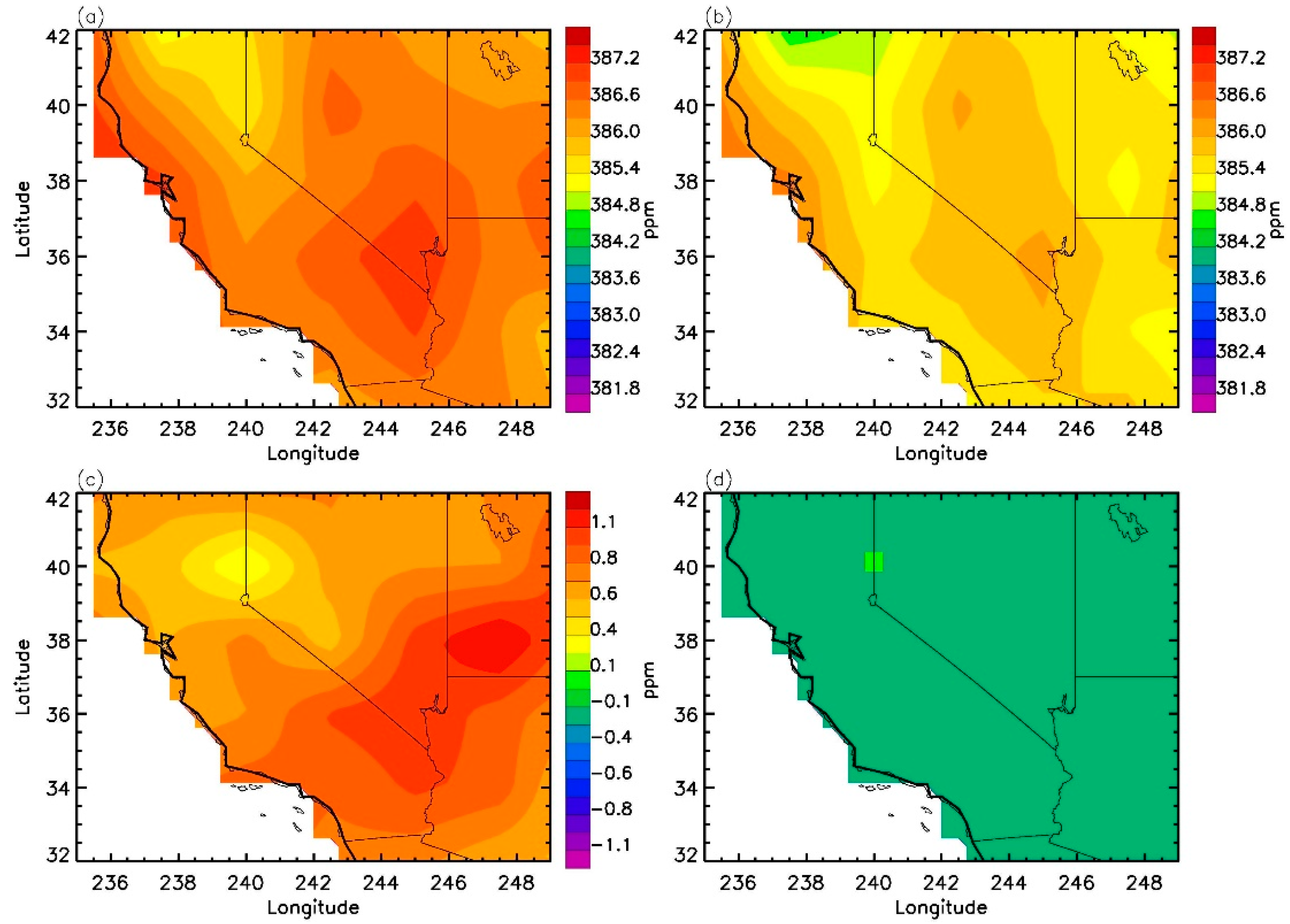
Figure 3.
(a) The mean value of 500 hPa vertical pressure velocity, from NCEP2, in dry years (JJAS of 2003, 2007, and 2010); (b) the mean value of 500 hPa vertical pressure velocity in wet years (JJAS of 2006, 2008, 2011, and 2012); (c) 500 hPa vertical pressure velocity differences between the dry and wet years; and (d) vertical pressure velocity differences within 5% significance level and 1% significance level are highlighted in light green and dark green. Units for Vertical pressure velocity are 10−2 Pa/s in (a–c).

Figure 4.
(a) The mean value of Net Ecosystem CO2 Exchange (NEE), from the CASA model, in dry years (JJAS of 2003, 2007, and 2010); (b) the mean value of NEE in wet years (JJAS of 2006, 2008, 2011, and 2012); (c) NEE differences between the dry and wet years; and (d) NEE differences within 5% significance level and 1% significance level are highlighted in light green and dark green. Units for NEE are g C m−2 mon−1 in (a–c).

© 2017 by the authors. Licensee MDPI, Basel, Switzerland. This article is an open access article distributed under the terms and conditions of the Creative Commons Attribution (CC BY) license (http://creativecommons.org/licenses/by/4.0/).
Share and Cite
MDPI and ACS Style
Jiang, X.; Kao, A.; Corbett, A.; Olsen, E.; Pagano, T.; Zhai, A.; Newman, S.; Li, L.; Yung, Y. Influence of Droughts on Mid-Tropospheric CO2. Remote Sens. 2017, 9, 852. https://doi.org/10.3390/rs9080852
AMA Style
Jiang X, Kao A, Corbett A, Olsen E, Pagano T, Zhai A, Newman S, Li L, Yung Y. Influence of Droughts on Mid-Tropospheric CO2. Remote Sensing. 2017; 9(8):852. https://doi.org/10.3390/rs9080852
Chicago/Turabian StyleJiang, Xun, Angela Kao, Abigail Corbett, Edward Olsen, Thomas Pagano, Albert Zhai, Sally Newman, Liming Li, and Yuk Yung. 2017. "Influence of Droughts on Mid-Tropospheric CO2" Remote Sensing 9, no. 8: 852. https://doi.org/10.3390/rs9080852
Note that from the first issue of 2016, this journal uses article numbers instead of page numbers. See further details here.