
Design and Simulation of Flexible Underwater Acoustic Sensor Based on 3D Buckling Structure

 , , and
Abstract
:1. Introduction
2. Technical Background
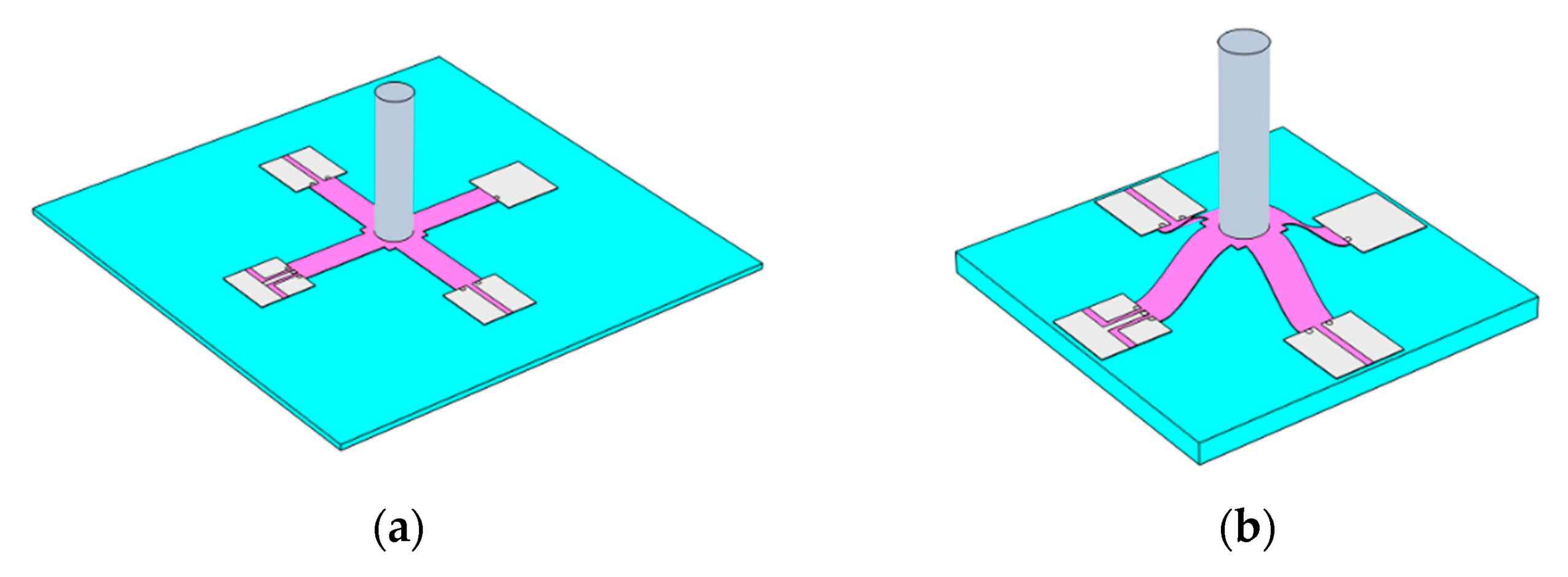
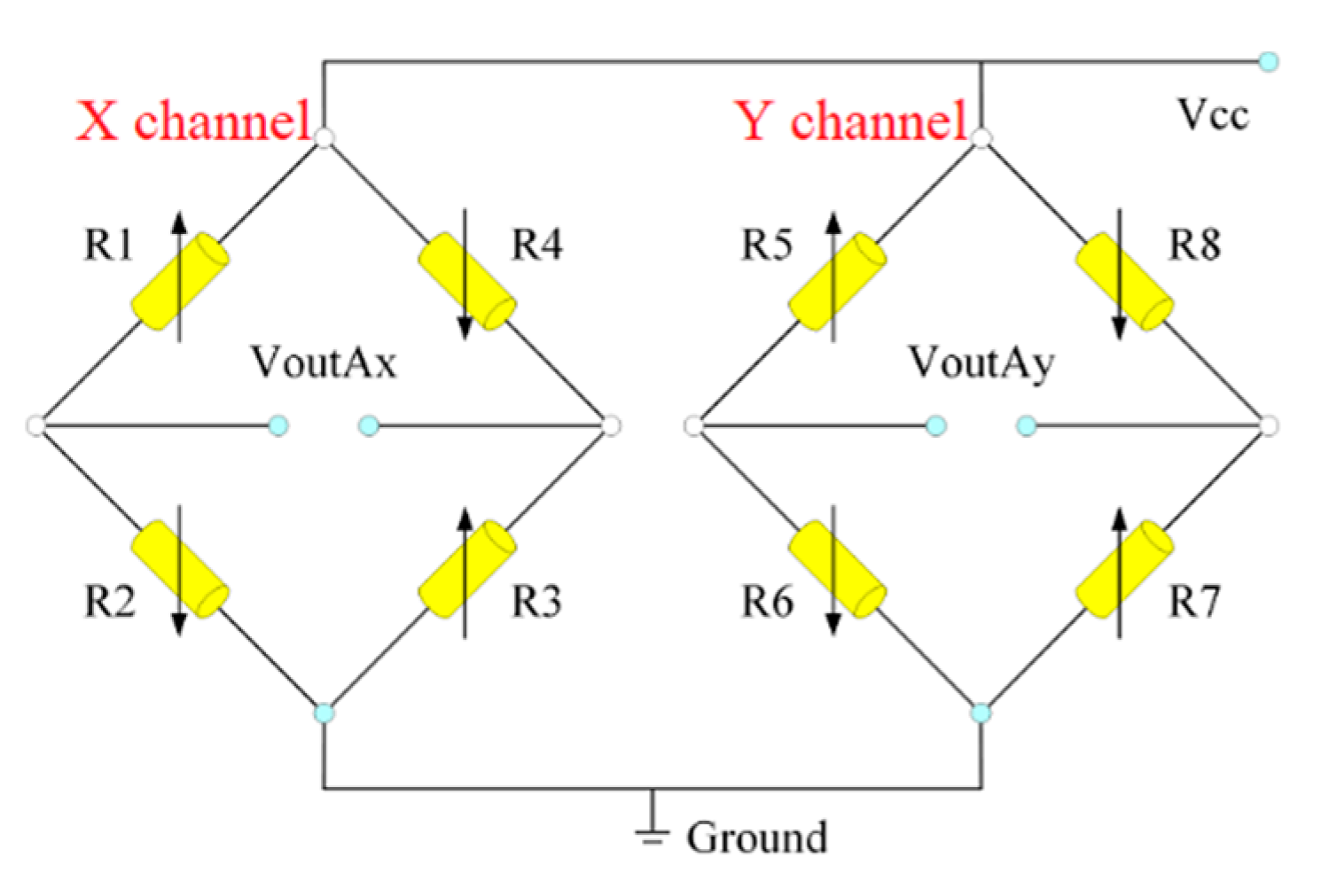
2.1. Working Principle
2.2. Fabrication Process
2.3. Physical-Field Interfaces
2.3.1. Solid Mechanics Interface
2.3.2. Pressure Acoustics–Frequency Domain Interface
2.3.3. Acoustics–Structure Interface
3. Methodology
3.1. Geometry and Materials
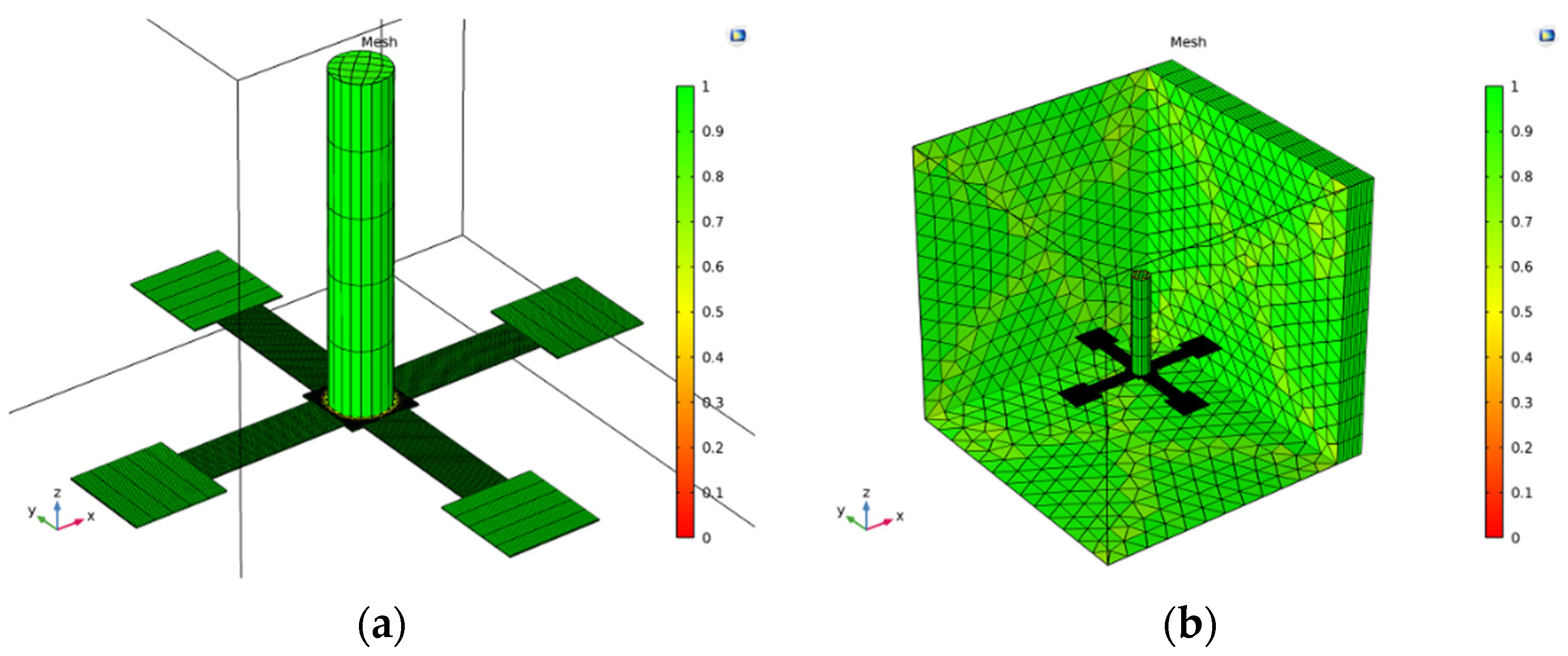
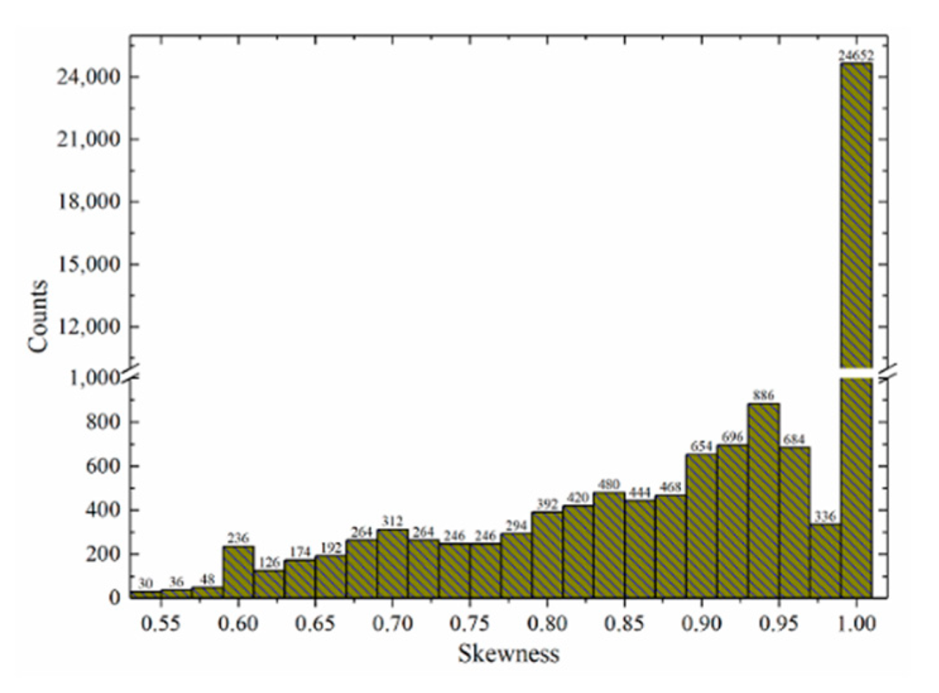
3.2. Mesh
4. Results and Discussions
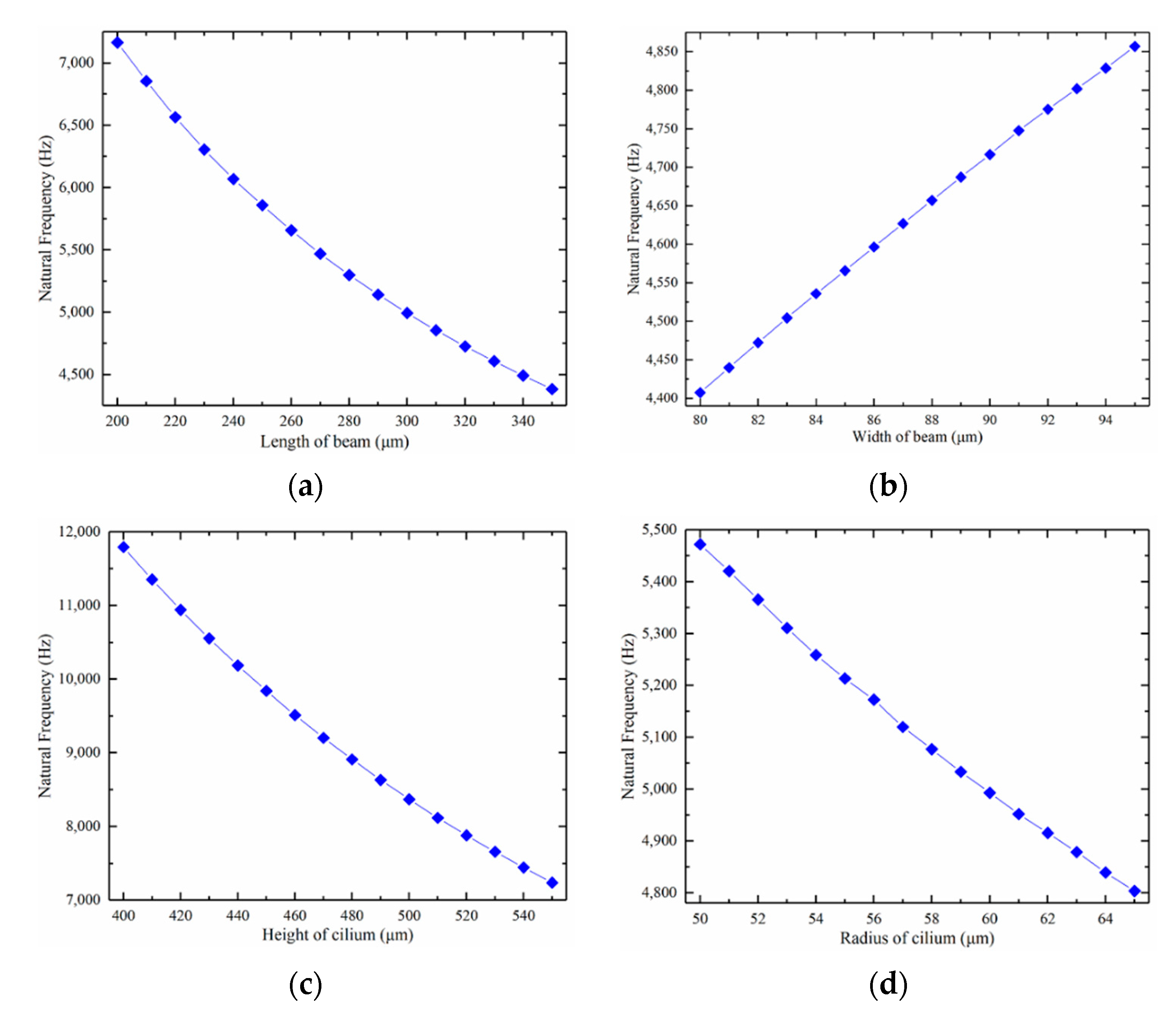
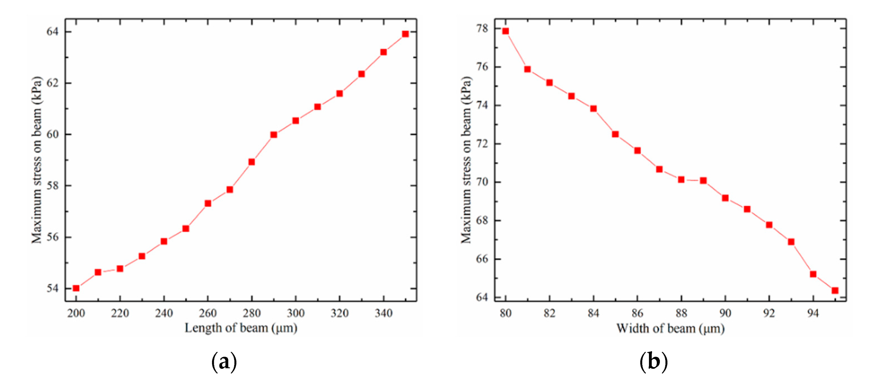
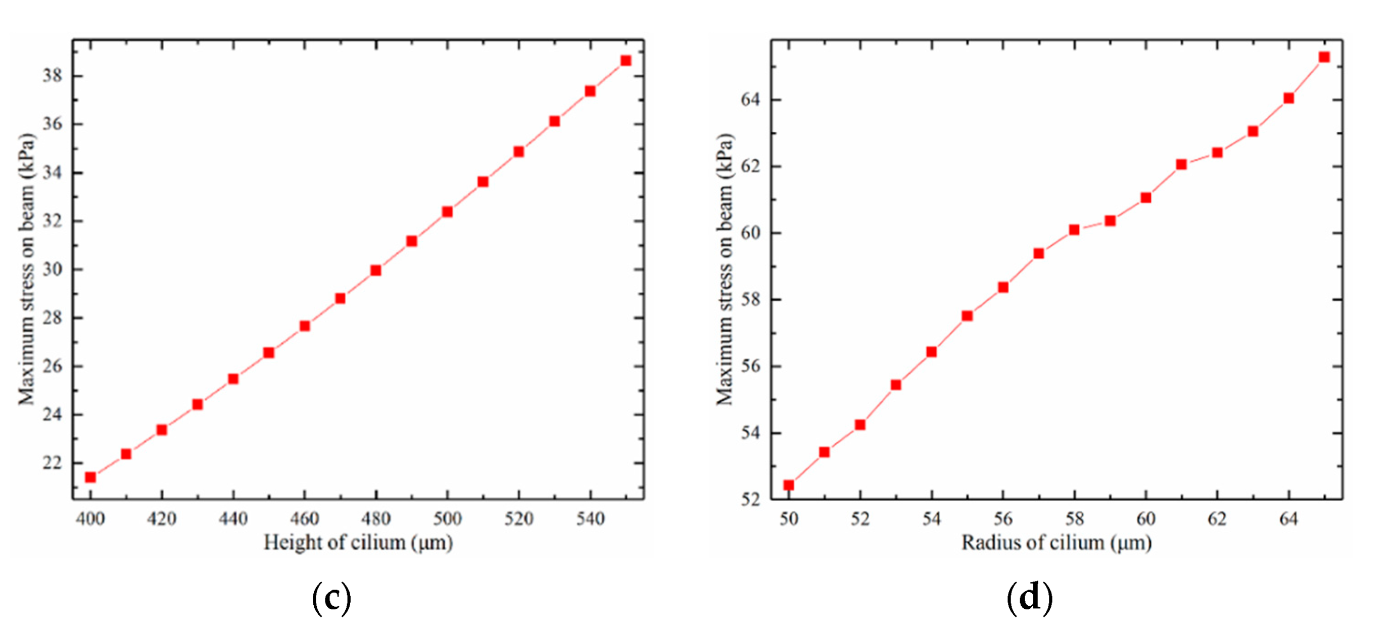
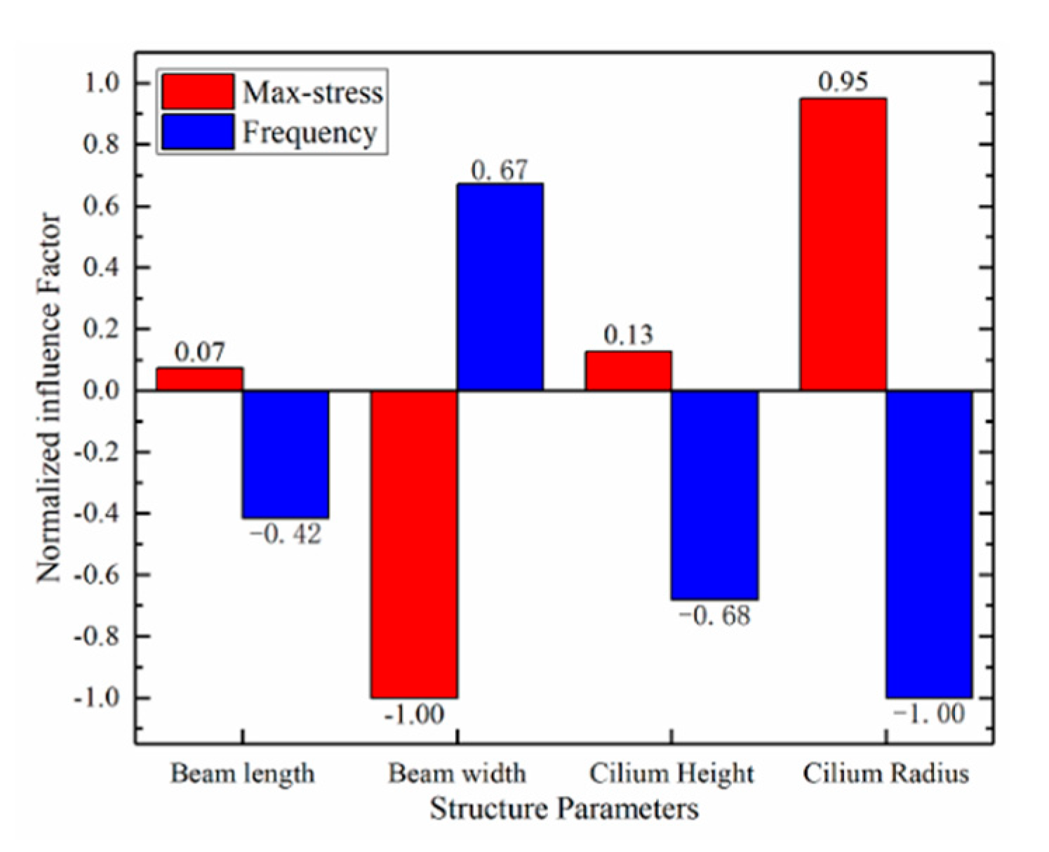
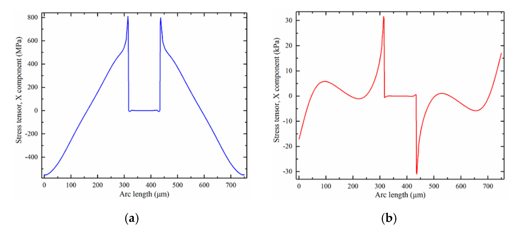
4.1. Natural Frequency and Stress
4.2. Sensitivity
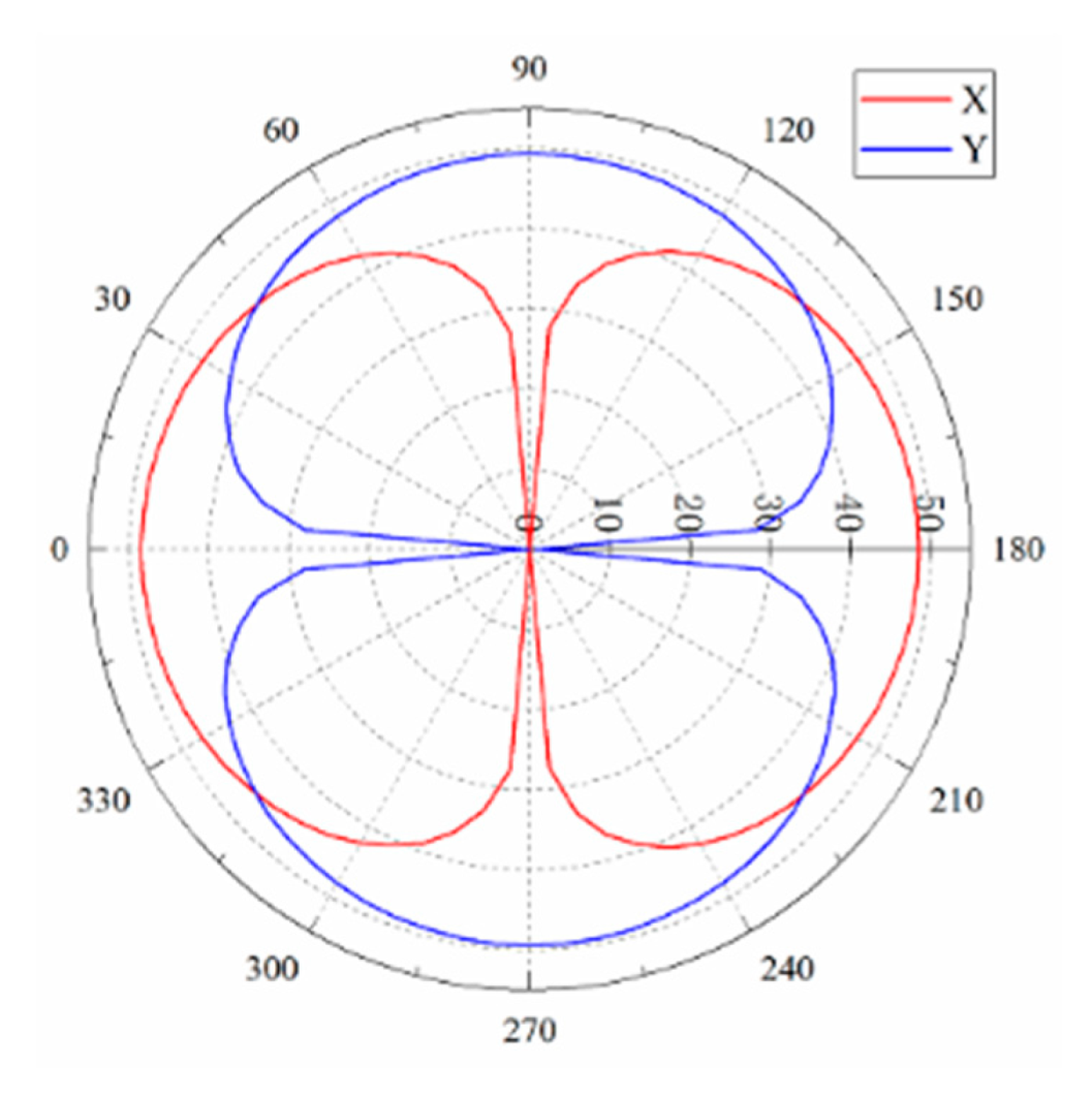
4.3. Directivity
5. Conclusions
Author Contributions
Funding
Data Availability Statement
Acknowledgments
Conflicts of Interest
References
- Yang, N.S. Development trends and implication in marine engineering and technology. Strateg. Study Chin. Acad. Eng. 2016, 18, 126–130. [Google Scholar] [CrossRef]
- Urick, R.J. Principles of Underwater Sound for Engineers, 3rd ed.; McGraw-Hill: New York, NY, USA, 1983. [Google Scholar]
- Nehorai, A.; Paldi, E. Vector-sensor array processing for electromagnetic source localization. IEEE. T. Signal. Proces. 1994, 42, 376–398. [Google Scholar] [CrossRef]
- Abraham, B.M. Low-cost dipole hydrophone for use in towed arrays. Am. Inst. Phys. 1996, 42, 376–398. [Google Scholar] [CrossRef]
- McConnell, J.A. Analysis of a compliantly suspended acoustic velocity sensor. J. Acoust. Soc. Am. 2003, 113, 1395–1405. [Google Scholar] [CrossRef] [PubMed]
- Rockstad, H.K.; Kenny, T.W.; Kelly, P.J.; Gabrielson, T.B. A microfabricated electron—Tunneling accelerometer as a directional underwater acoustic sensor. AIP Conf. Proc. 1996, 368, 57–68. [Google Scholar] [CrossRef]
- Xue, C.Y.; Chen, S.; Zhang, W.D.; Zhang, B.Z.; Zhang, G.J.; Qiao, H. Design, fabrication, and preliminary characterization of a novel MEMS bionic vector hydrophone. Microelectron. J. 2007, 38, 1021–1026. [Google Scholar] [CrossRef]
- Shi, F.; Ramesh, P.; Mukherjee, S. Simulation methods for micro-electro-mechanical structures (MEMS) with application to a microtweezer. Comput. Struct. 1995, 56, 769–783. [Google Scholar] [CrossRef]
- Chen, L.J.; Yang, S.E. A design of novel piezoresistive vector hydrophone. Appl. Acoust. 2006, 25, 273–278. [Google Scholar]
- Liu, Y.; Wang, R.X.; Zhang, G.J.; Du, J.; Zhao, L.; Xue, C.Y.; Zhang, W.D.; Liu, J. “Lollipop-shaped” high-sensitivity Microelectromechanical Systems vector hydrophone based on Parylene encapsulation. J. Appl. Phys. 2015, 118, 7. [Google Scholar] [CrossRef]
- Xu, Q.D.; Zhang, G.J.; Ding, J.W.; Wang, R.X.; Pei, Y.; Ren, Z.M.; Shang, Z.Z.; Xue, C.Y.; Zhang, W.D. Design and implementation of two-component cilia cylinder MEMS vector hydrophone. Sens. Actuator A-Phys. 2018, 277, 142–149. [Google Scholar] [CrossRef]
- Ji, S.X.; Zhang, L.S.; Zhang, W.D.; Zhang, G.J.; Wang, R.X.; Song, J.L.; Zhang, X.Y.; Lian, Y.Q.; Shang, Z.Z. Design and realization of dumbbell-shaped ciliary MEMS vector hydrophone. Sens. Actuator A-Phys. 2020, 311, 9. [Google Scholar] [CrossRef]
- Yang, X.; Xu, Q.D.; Zhang, G.J.; Zhang, L.S.; Wang, W.D.; Shang, Z.Z.; Shi, Y.M.; Li, C.G.; Wang, R.X.; Zhang, W.D. Design and implementation of hollow cilium cylinder MEMS vector hydrophone. Measurement 2021, 168, 7. [Google Scholar] [CrossRef]
- Wang, R.X.; Liu, Y.; Xu, W.; Bai, B.; Zhang, G.J.; Liu, J.; Xiong, J.J.; Zhang, W.D.; Xue, C.Y.; Zhang, B.Z. A ‘fitness-wheel-shaped’ MEMS vector hydrophone for 3D spatial acoustic orientation. J. Micromech. Microeng. 2017, 27, 8. [Google Scholar] [CrossRef]
- Xu, W.; Liu, Y.; Zhang, G.J.; Wang, R.X.; Xue, C.Y.; Zhang, W.D.; Liu, J. Development of cup-shaped micro-electromechanical systems-based vector hydrophone. J. Appl. Phys. 2016, 120, 8. [Google Scholar] [CrossRef]
- Wang, R.X.; Shen, W.; Zhang, W.J.; Song, J.L.; Li, N.S.; Liu, M.R.; Zhang, G.J.; Xue, C.Y.; Zhang, W.D. Design and implementation of a jellyfish otolith-inspired MEMS vector hydrophone for low-frequency detection. Microsyst. Nanoeng. 2021, 7, 10. [Google Scholar] [CrossRef] [PubMed]
- Kim, J.; Lee, M.; Shim, H.J.; Ghaffari, R.; Cho, H.R.; Son, D.; Jung, Y.H.; Soh, M.; Choi, C.; Jung, S.; et al. Stretchable silicon nanoribbon electronics for skin prosthesis. Nat. Commun. 2014, 5, 11. [Google Scholar] [CrossRef] [PubMed] [Green Version]
- Cho, M.; Yun, J.; Kwon, D.; Kim, K.; Park, I. High-Sensitivity and Low-Power Flexible Schottky Hydrogen Sensor Based on Silicon Nanomembrane. ACS Appl. Mater. Interfaces 2018, 10, 12870–12877. [Google Scholar] [CrossRef] [PubMed]
- Li, G.J.; Song, E.M.; Huang, G.S.; Pan, R.B.; Guo, Q.L.; Ma, F.; Zhou, B.; Di, Z.F.; Mei, Y.F. Flexible Transient Phototransistors by Use of Wafer-Compatible Transferred Silicon Nanomembranes. Small 2018, 14. [Google Scholar] [CrossRef] [PubMed]
- Khang, D.Y.; Jiang, H.Q.; Huang, Y.; Rogers, J.A. A stretchable form of single-crystal silicon for high-performance electronics on rubber substrates. Science 2006, 311, 208–212. [Google Scholar] [CrossRef] [PubMed] [Green Version]
- Xu, S.; Yan, Z.; Jang, K.I.; Huang, W.; Fu, H.R.; Kim, J.; Wei, Z.; Flavin, M.; McCracken, J.; Wang, R.; et al. Assembly of micro/nanomaterials into complex, three-dimensional architectures by compressive buckling. Science 2015, 347, 154–159. [Google Scholar] [CrossRef] [PubMed] [Green Version]
- Qiao, H.; Liu, J.; Zhang, B.Z.; Zhang, W.D.; Xue, C.Y. Actuators. Design of a novel Si-based bionic vector hydrophone based on piezoresistive effect. Chin. J. Sens. 2008, 21, 301–304. [Google Scholar]
- Xu, Q.D.; Zhang, G.J.; Zhao, Y.J.; Wang, R.X.; Ding, J.W.; Zhang, X.Y.; Xue, C.Y.; Zhang, W.D. New insight into contradictive relationship between sensitivity and working bandwidth of cilium MEMS bionic vector hydrophone. J. Micromech. Microeng. 2019, 29, 11. [Google Scholar] [CrossRef]
- Zimmerman, W.B.J. Multiphysics Modeling with Finite Element Methods; World Scientific: Singapore, 1983. [Google Scholar]
- Liu, Y.; Wang, X.J.; Xu, Y.M.; Xue, Z.G.; Zhang, Y.; Ning, X.; Chen, X.; Xue, Y.G.; Lu, D.; Zhang, Q.H.; et al. Harnessing the interface mechanics of hard films and soft substrates for 3D assembly by controlled buckling. Proc. Natl. Acad. Sci. USA 2019, 116, 15368–15377. [Google Scholar] [CrossRef] [PubMed] [Green Version]


| Material | Young’s Modulus (GPa) | Poisson’s Ratio | Density (kg/m3) | Sound Velocity (m/s) |
|---|---|---|---|---|
| Si | 130 | 0.27 | 2329 | / |
| SiO2 | 70 | 0.2 | 2200 | / |
| Structure Name | Parameter (μm) |
|---|---|
| Length of the crossbeam | 300 |
| Width of the crossbeam | 100 |
| Thickness of the crossbeam | 3 |
| Length of the pad’s side | 200 |
| Length of the central block’s side | 150 |
| Height of the cilium | 700 |
| Radius of the cilium | 60 |
Publisher’s Note: MDPI stays neutral with regard to jurisdictional claims in published maps and institutional affiliations. |
© 2021 by the authors. Licensee MDPI, Basel, Switzerland. This article is an open access article distributed under the terms and conditions of the Creative Commons Attribution (CC BY) license (https://creativecommons.org/licenses/by/4.0/).
Share and Cite
Liu, G.; Cao, W.; Zhang, G.; Wang, Z.; Tan, H.; Miao, J.; Li, Z.; Zhang, W.; Wang, R. Design and Simulation of Flexible Underwater Acoustic Sensor Based on 3D Buckling Structure. Micromachines 2021, 12, 1536. https://doi.org/10.3390/mi12121536
Liu G, Cao W, Zhang G, Wang Z, Tan H, Miao J, Li Z, Zhang W, Wang R. Design and Simulation of Flexible Underwater Acoustic Sensor Based on 3D Buckling Structure. Micromachines. 2021; 12(12):1536. https://doi.org/10.3390/mi12121536
Chicago/Turabian StyleLiu, Guochang, Wenping Cao, Guojun Zhang, Zhihao Wang, Haoyu Tan, Jinwei Miao, Zhaodong Li, Wendong Zhang, and Renxin Wang. 2021. "Design and Simulation of Flexible Underwater Acoustic Sensor Based on 3D Buckling Structure" Micromachines 12, no. 12: 1536. https://doi.org/10.3390/mi12121536