Effective Permittivity for FDTD Calculation of Plasmonic Materials

Abstract

We present a new effective permittivity (EP) model to accurately calculate surface plasmons (SPs) using the finite-difference time-domain (FDTD) method. The computational representation of physical structures with curved interfaces causes inherent errors in FDTD calculations, especially when the numerical grid is coarse. Conventional EP models improve the errors, but they are not effective for SPs because the SP resonance condition determined by the original permittivity is changed by the interpolated EP values. We perform FDTD simulations using the proposed model for an infinitely-long silver cylinder and gold sphere, and the results are compared with Mie theory. Our model gives better accuracy than the conventional staircase and EP models for SPs.

1. Introduction

Surface plasmons (SPs) are waves that propagate along the surface of a metal and play a role in subwavelength imaging [1]. SPs have been applied to advanced optical devices, for example, sensors, microscopies, lasers, invisibility cloaks, and hyperlenses [2,3,4,5,6,7,8,9]. Numerical simulations are useful to analyze the complicated structures of these devices. In this paper, we discuss a finite-difference time-domain (FDTD) analysis of the SP. The FDTD method has gained popularity because of several reasons: it is easy to implement, it works in the time domain, and arbitrary shapes can be calculated [10,11,12,13]. However, there are inherent errors in the FDTD method caused by numerical dispersion, the absorbing boundary condition, and the permittivity model. The former two can be improved by using the nonstandard FDTD method [14] and the perfectly matched layer [13]. We address the error of the permittivity model. On a discrete grid, it is difficult to model permittivity interfaces that run between the grid points. The permittivity interface model is often an accuracy bottleneck, especially when the SPs are calculated on a coarse grid. By improving the model, we can accurately calculate optical effects on a coarse grid with a low computational cost.

The permittivity model error has been reduced by various approaches. The conformal FDTD method on non-orthogonal grids [15,16,17], counter path FDTD method [18,19], and subgridding method [20,21,22] can represent curved interfaces suitably, but they are relatively difficult to implement and increase the memory and computation time. A different approach using effective permittivities (EPs), which derives from interface interpolations based on Ampere’s and Faraday’s integration laws, can reduce the error of the permittivity model on coarse grids in a simple implementation and at low computational cost [23,24,25,26,27,28,29,30,31,32,33,34,35]. The EP method, however, is not effective for plasmonic materials because the SP resonance condition is changed on interfaces due to interpolated values of EPs. Plasmonic waveguides have been analyzed by the conformal FDTD method using EPs [36], but the SP resonance wavelength is shifted several nanometers even on a fine grid (wavelength/grid spacing = 60). Furthermore, this method involves a complicated implementation given by a fourth-order differential equation. Ultimately, permittivities must be staircased to capture the correct SP resonance condition.

In this paper we propose a modified EP model to accurately calculate SP resonances on a coarse grid. A key concept is that the permittivities of plasmonic materials are used not only inside the materials but also on grid points adjacent to the materials (discussed in Section 2). In Section 3, numerical simulations for an infinitely-long silver cylinder and a gold sphere demonstrate that our model is in better agreement with Mie theory than the conventional staircase and EP models.

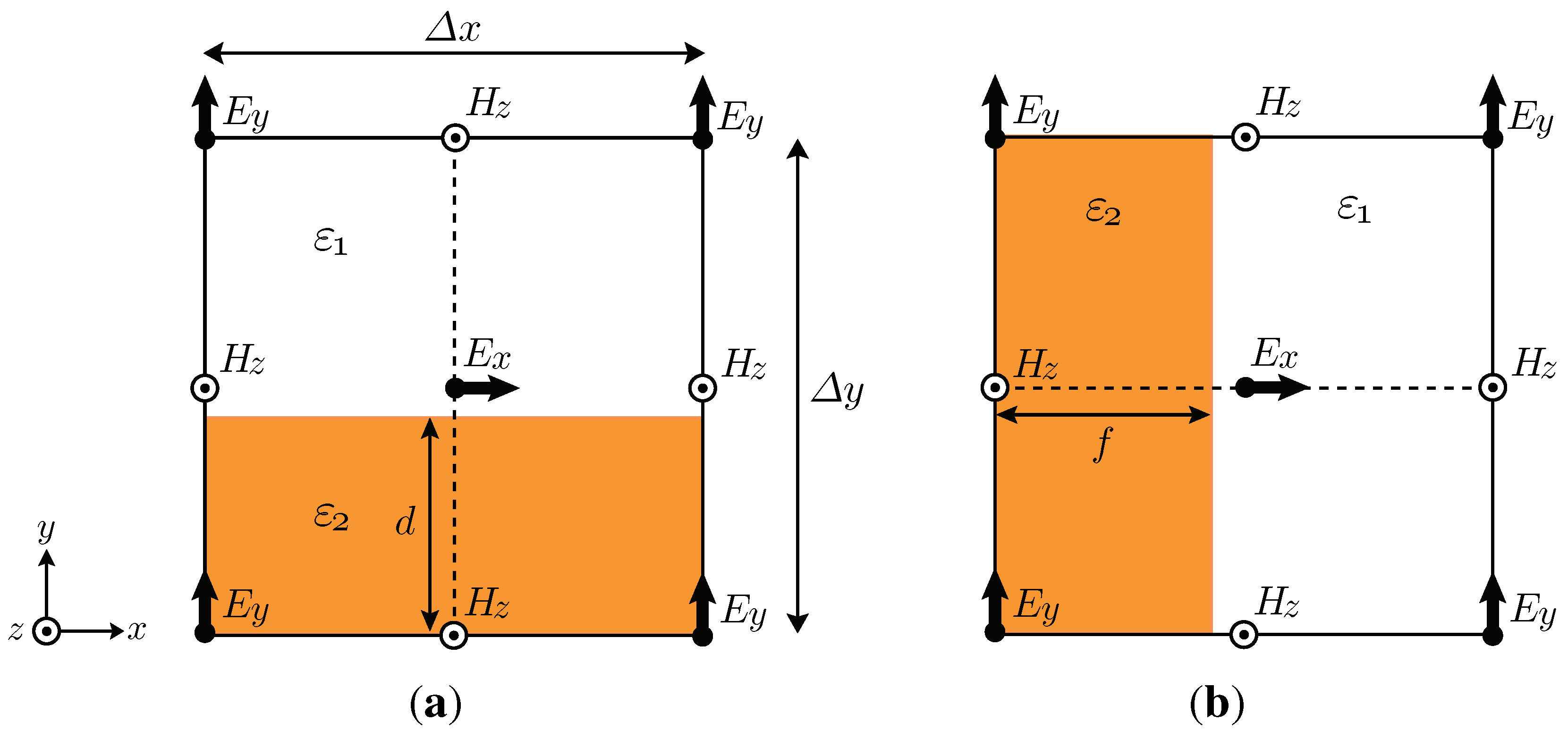
2. Effective Permittivity for Plasmonic Materials

Permittivities of plasmonic materials must be staircased, because the SP resonance condition given by interpolated EPs on interfaces is different from that of the original metal permittivity. But the staircase model is too crude to give high accuracy. Regardless of how close it lies to the interface, a grid point is either “in” or “out”. The key to improve the representation is to take distance from the interface into account when assigning an permittivity value to a grid point.

In order to introduce our model, we start by analyzing EPs for plasmonic materials in the two-dimensional transverse magnetic (TM) mode, in which the electromagnetic fields reduce to three non-zero components $E_x$, $E_y$, and $H_z$. Ampere’s and Faraday’s integration laws are given by

$$\begin{array}{c}\hfill \frac{\partial }{\partial t}\int \mathbf{D}·d\mathbf{S}=\oint \mathbf{H}·d\mathbf{l}\end{array}$$

(1)

$$\begin{array}{c}\hfill -\frac{\partial }{\partial t}\int \mathbf{B}·d\mathbf{S}=\oint \mathbf{E}·d\mathbf{l}\end{array}$$

(2)

where $\mathbf{E}$ is the electric field, $\mathbf{D}$ is the electric induction, $\mathbf{H}$ is the magnetic field, $\mathbf{B}$ is the magnetic induction, $d\mathbf{S}$ is an element of surface area, and $d\mathbf{l}$ is an infinitesimal length element. Figure 1 shows examples of partially filled FDTD cells in the TM mode: (a) interface parallel to $E_x$; (b) interface perpendicular to $E_x$, where $\mathsf{\Delta }x,\mathsf{\Delta }y$ are grid spacings, $d,f$ are filling factors on the integration lines, and ${\epsilon }_1,{\epsilon }_2$ are permittivities outside and inside the plasmonic material, respectively. In Figure 1(a), Ampere’s law gives an integration with respect to the $E_x$ components:

$${\int }_{y-\mathsf{\Delta }y/2}^{y+\mathsf{\Delta }y/2}{D}_x(x,y)dy={\int }_{y-\mathsf{\Delta }y/2}^{y-\mathsf{\Delta }y/2+d}{D}_x(x,y)dy+{\int }_{y-\mathsf{\Delta }y/2+d}^{y+\mathsf{\Delta }y/2}{D}_x(x,y)dy$$

(3)

Assuming $\mathsf{\Delta }y$ to be sufficiently small, $D_x$ and $E_x$ are essentially constant in the integration region. Since $E_x$ parallel to the interface is continuous on each plane, substituting $D_x={\epsilon }_{\Vert }{E}_x$ (${\epsilon }_{\Vert }=$ EP for Ampere’s law) into the left-hand side of Equation (3), we obtain

$${\epsilon }_{\Vert }=(d/\mathsf{\Delta }y){\epsilon }_2+\left(1-d/\mathsf{\Delta }y\right){\epsilon }_1$$

(4)

In Figure 1(b), Faraday’s law gives the other integration:

$$\begin{array}{c}\hfill \begin{array}{cc}\hfill {\int }_{x-\mathsf{\Delta }x/2}^{x+\mathsf{\Delta }x/2}[E_x(x,y-h/2)& -E_x(x,y+h/2)]dx\hfill \\ \hfill & ={\int }_{x-\mathsf{\Delta }x/2}^{x-\mathsf{\Delta }x/2+f}\left[E_x(x,y-h/2)-E_x(x,y+h/2)\right]dx\hfill \\ \hfill & +{\int }_{x-\mathsf{\Delta }x/2+f}^{x+\mathsf{\Delta }x/2}\left[E_x(x,y-h/2)-E_x(x,y+h/2)\right]dx\hfill \end{array}\end{array}$$

(5)

Since the $D_x$ perpendicular to the interface is continuous, ${\epsilon }_1{E}_x={\epsilon }_2{E}_x$ on the interface. If we assume

$${\int }_{x-\mathsf{\Delta }x/2}^{x-\mathsf{\Delta }x/2+f}{\epsilon }_2{E}_x(x,y)dx={\int }_{x-\mathsf{\Delta }x/2+f}^{x+\mathsf{\Delta }x/2}{\epsilon }_1{E}_x(x,y)dx$$

(6)

similarly we can obtain the EP for Faraday’s law:

$${\epsilon }_{\perp }=\frac{1}{(f/\mathsf{\Delta }x)/{\epsilon }_2+\left(1-f/\mathsf{\Delta }y\right)/{\epsilon }_1}$$

(7)

Detailed derivations of ${\epsilon }_{\Vert }$ and ${\epsilon }_{\perp }$ are given in [23,24,25,26,27,28].

The ${\epsilon }_{\Vert }$ and ${\epsilon }_{\perp }$ models give high accuracy for non-plasmonic materials on a coarse grid, however, they are not effective for plasmonic ones. Figure 2 shows (a) propagating and (b) localized SPs. In Figure 2, strongly resonant SP fields enclosed with dotted lines are in the polarization perpendicular to the interface. The ${\epsilon }_{\perp }$ model fits this situation, but the approximation of Equation (6) is invalid because the SP decays exponentially with increasing distance from the metal surface. On the other hand, the damping has only a small effect for the low power parallel field, and the ${\epsilon }_{\Vert }$ model can be used. However, the permittivity values must be staircased in order to preserve the resonance condition as discussed before.

We empirically found that the SP resonances can be accurately calculated by staircasing the ${\epsilon }_{\Vert }$ model in the following manner:

$${\epsilon }_{\mathrm{EP}}=\left\{\begin{array}{cc}{\epsilon }_2,\hfill & \mathrm{for} d>0\hfill \\ {\epsilon }_1,\hfill & \mathrm{otherwise}\hfill \end{array}\right.$$

(8)

for both the parallel and perpendicular cases. Equation (8) represents what we call the staircased EP (S-EP) model. In the S-EP model, even when the $E_x$ grid point is outside the plasmonic medium (${\epsilon }_2$) as shown in Figure 1(a), it is assigned to the value ${\epsilon }_2$ if $d>0$. When the $E_x$ is perpendicular to the interface as shown in Figure 1(b), the conventional staircase model is used because $d=0$ or 1. Equation (8) is applied to the $E_x$ grid points, but the $E_y$ assignments can be obtained with the same procedure. The S-EP model can be simply implemented in Yee Algorithm [10,11,12,13]:

$$\begin{array}{cc}\hfill E_x^{n+1}& =E_x^n+\frac{\mathsf{\Delta }t}{{\epsilon }_{\mathrm{EP}}h}{d}_y{H}_z^{n+1/2}\hfill \end{array}$$

(9)

$$\begin{array}{cc}\hfill E_y^{n+1}& =E_y^n-\frac{\mathsf{\Delta }t}{{\epsilon }_{\mathrm{EP}}h}{d}_x{H}_z^{n+1/2}\hfill \end{array}$$

(10)

$$\begin{array}{cc}\hfill H_z^{n+3/2}& =H_z^{n+1/2}-\frac{\mathsf{\Delta }t}{\mu h}\left(d_x{E}_y^{n+1}-d_y{E}_x^{n+1}\right)\hfill \end{array}$$

(11)

where $\mathsf{\Delta }t$ is the time interval, h is the grid spacing, ${\mu }_0$ is the permeability, and we simply write $D_x(t=n\mathsf{\Delta }t)\to D_x^n$ ($n=$ integer). The spatial difference operators $d_x$, $d_y$ are defined by

$$\begin{array}{cc}\hfill d_{x}f(x,y)& =f(x+h/2,y)-f(x-h/2,y)\hfill \end{array}$$

(12)

$$\begin{array}{cc}\hfill d_{y}f(x,y)& =f(x,y+h/2)-f(x,y-h/2)\hfill \end{array}$$

(13)

The S-EP model thus prescribes how to assign permittivity values to grid points near medium interfaces. In Section 3, we shown that the S-EP model is more accurate than the conventional staircase and EP models. This method can be readily extended to three dimensions, keeping in mind that the line integrals become surface integrals in Ampere’s law.

3. Numerical Validations

We validate the S-EP model in FDTD simulations for an infinitely-long cylinder of silver (Ag) and sphere of gold (Au). Localized SPs are generated for wavelengths: >340 nm for the Ag cylinder; >510 nm for the Au sphere. FDTD results using the S-EP model are compared with those of the conventional staircase and EP models, and with Mie theory [37]. Since the ${\epsilon }_{\perp }$ model has a large error for SPs as discussed in Section 2, we employ the ${\epsilon }_{\Vert }$ model as a comparison. To analyze dispersive materials, we use the auxiliary differential equation method with the Drude Model (taking an example) [13]:

$$\epsilon =1-\frac{{\omega }_p^2}{{\omega }^2+i{\nu }_c\omega }$$

(14)

where ${\omega }_p$ is the plasma frequency, and ${\nu }_c$ is the collision frequency. To capture the measured permittivities of Johnson and Christy [38], we calculate ${\omega }_p,{\nu }_c$ at each wavelength as follows:

$$\begin{array}{cc}\hfill {\omega }_p& =\omega \sqrt{\frac{{\left(1-{\epsilon }_r\right)}^2+{\epsilon }_i^2}{1-{\epsilon }_r}}\hfill \end{array}$$

(15)

$$\begin{array}{cc}\hfill {\nu }_c& =\omega \left(\frac{{\epsilon }_i}{1-{\epsilon }_r}\right)\hfill \end{array}$$

(16)

where $\epsilon ={\epsilon }_r+i{\epsilon }_i$.

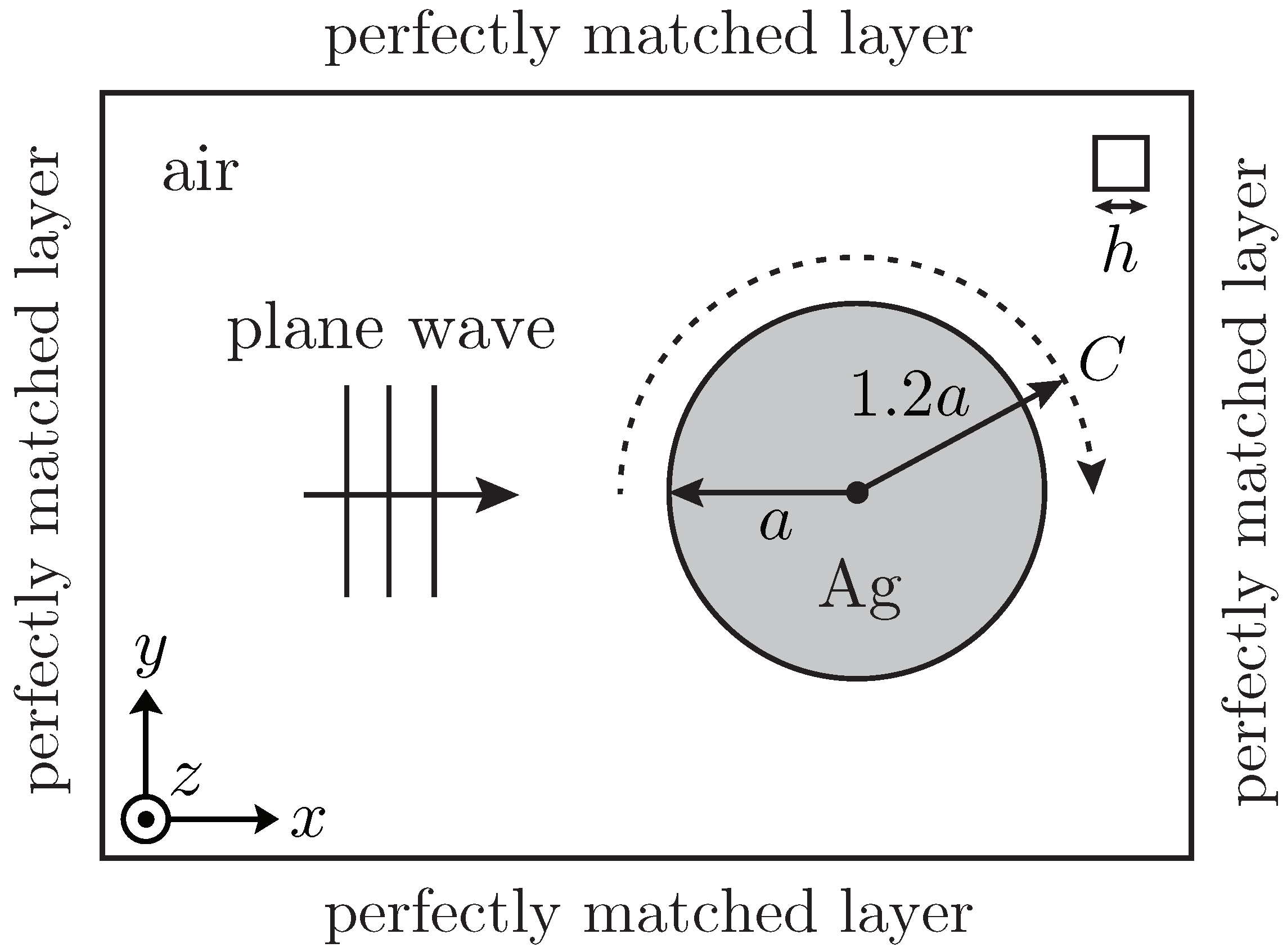
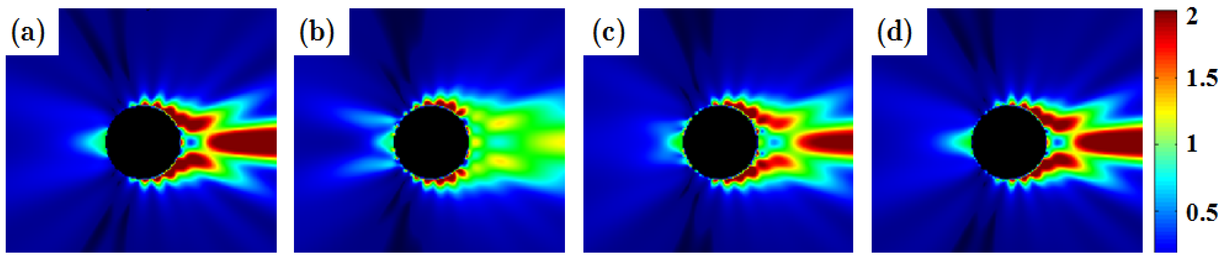
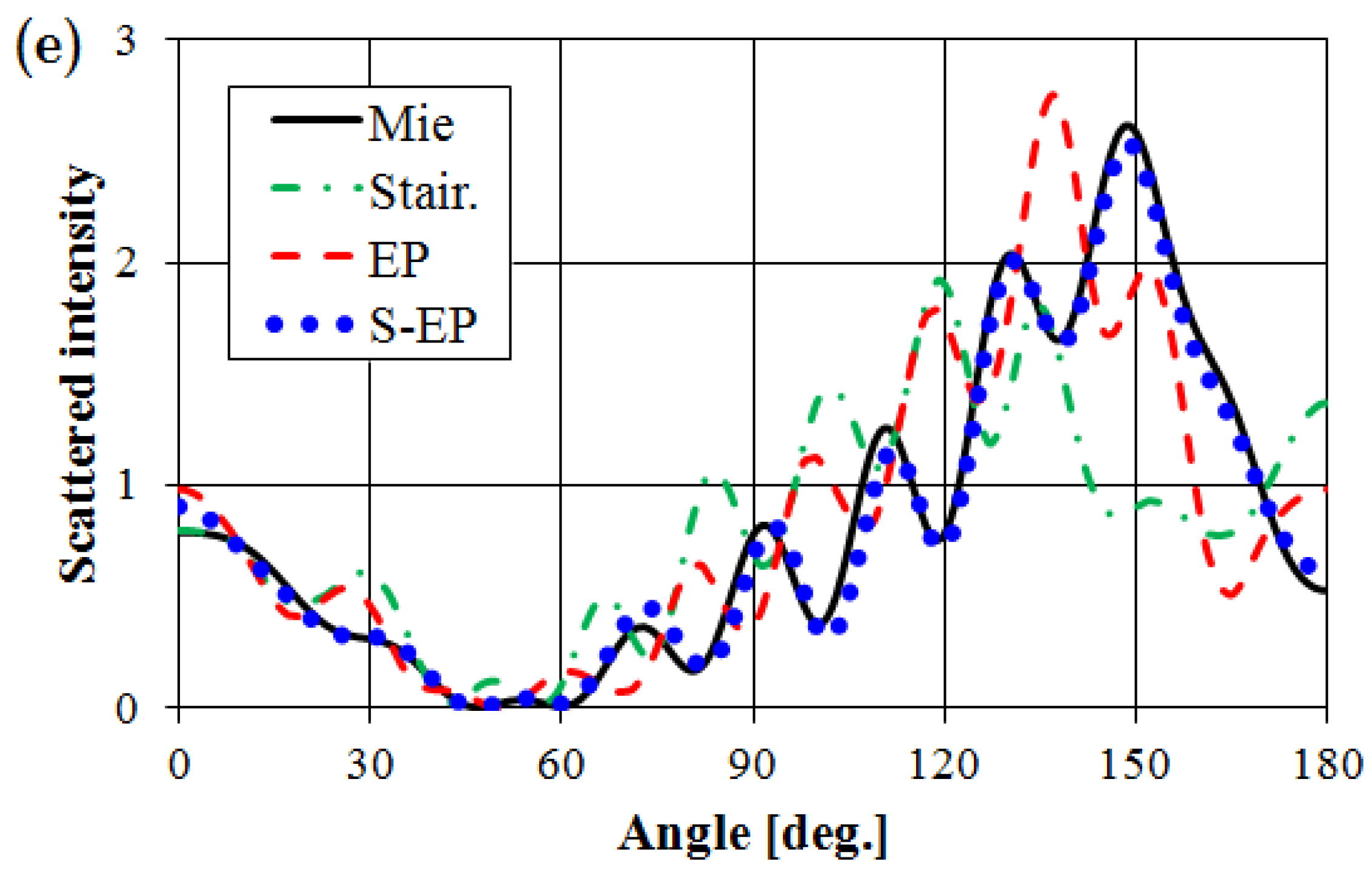
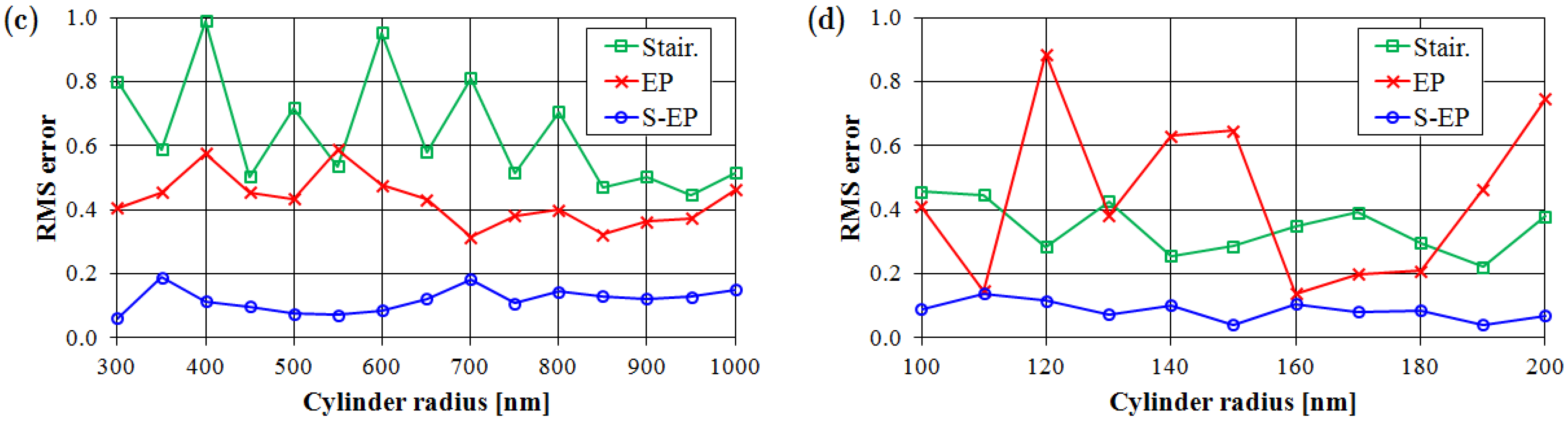
3.1. Infinitely-Long Ag Cylinder

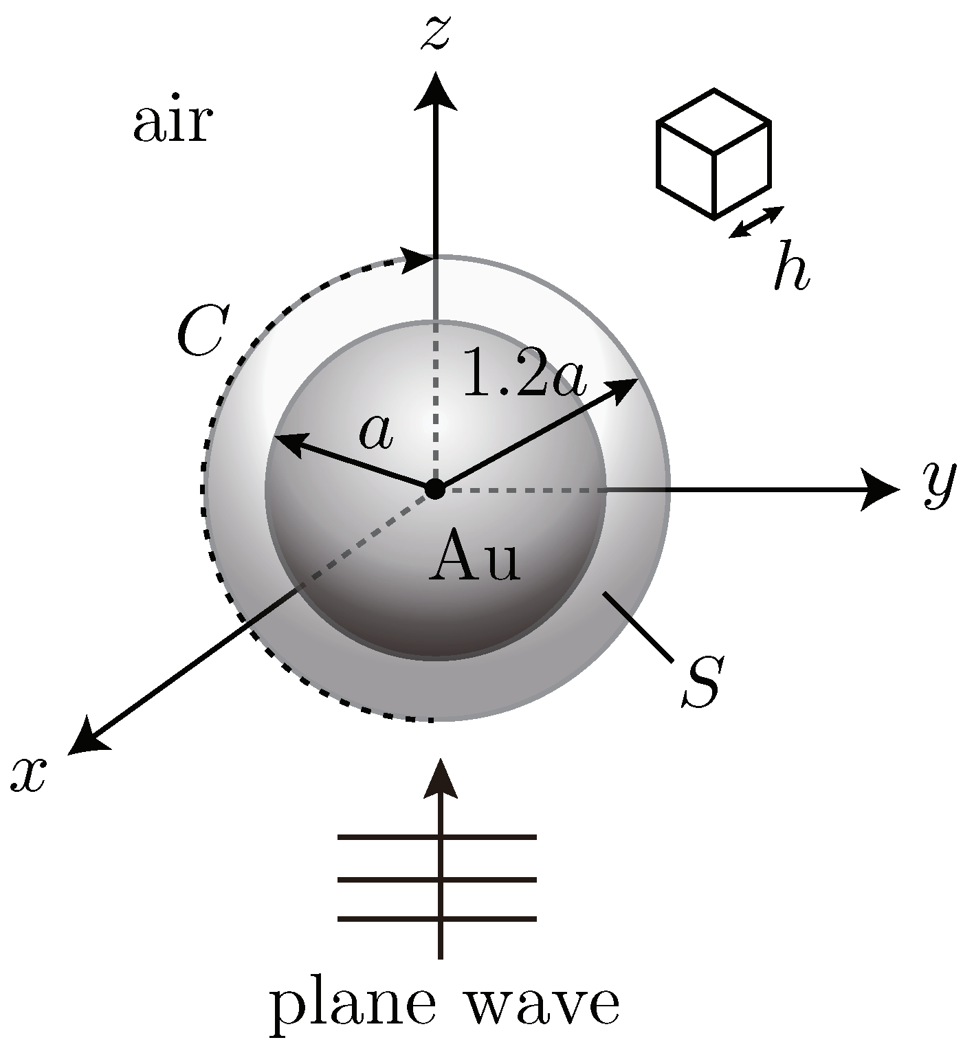
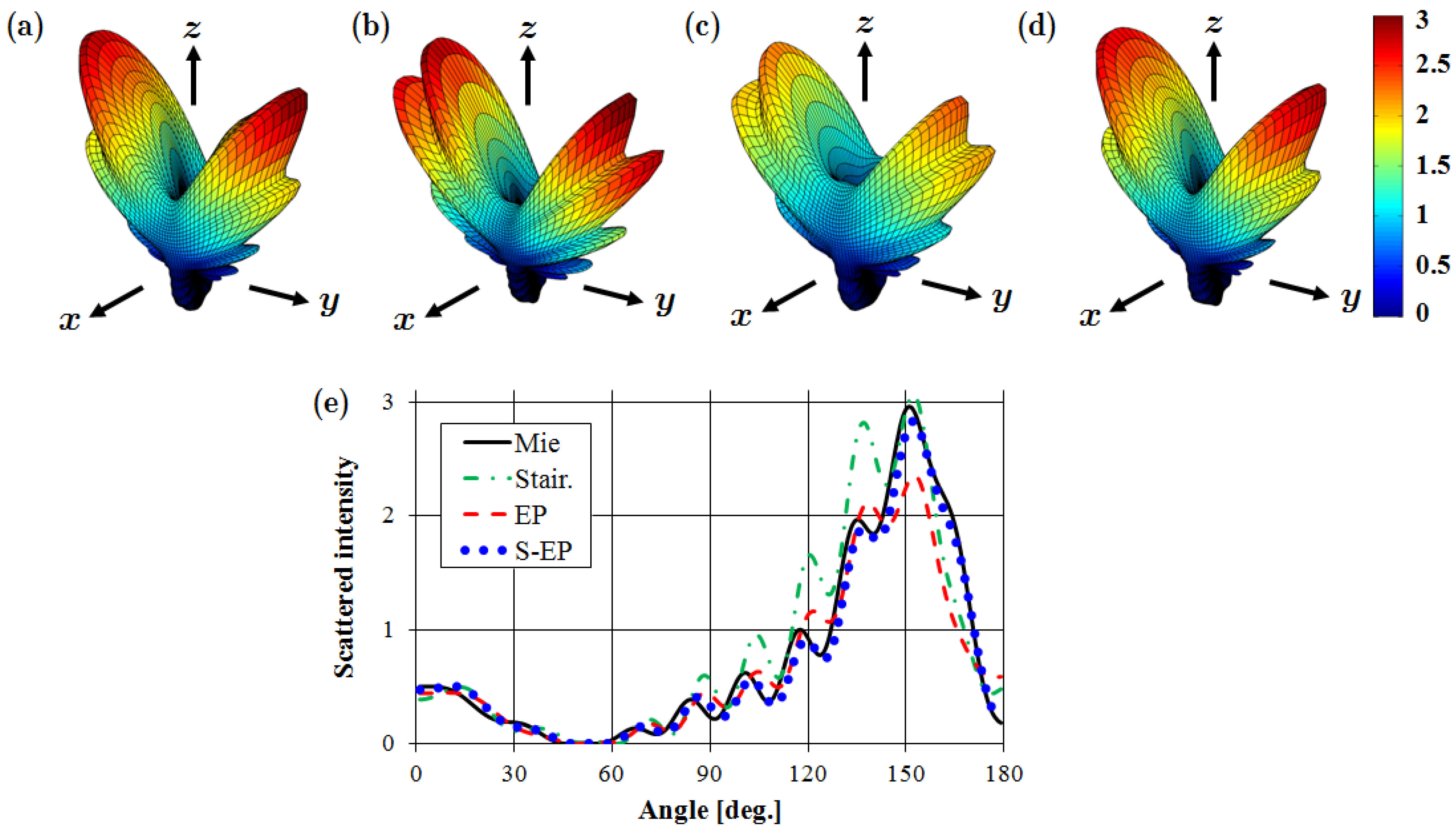
Figure 3 shows the simulation setup for an infinitely-long Ag cylinder: the computational domain is terminated by a perfectly matched layer (PML) [13]; a plane wave source of wavelength ${\lambda }_0=$ 430.501 nm (696 THz) in the SP waveband of Ag (>340 nm) is TM polarized; the cylinder radius is $a=1.25{\lambda }_0=$ 538.126 nm; the grid spacing is $h=$ 20 nm (${\lambda }_0/h=$ 21.5); and the time step is given by the Courant limit. FDTD calculations are compared with Mie theory on a contour C of radius $1.2a$ about the cylinder. Simulation parameters for the infinitely-long Ag cylinder are listed in

Table 1. Simulation parameters for an infinitely-long Ag cylinder.

Parameter	Input Value
permittivity of air ${\epsilon }_1$	1
permittivity of Ag ${\epsilon }_2$	−6.06 + i0.197
wavelength ${\lambda }_0$	430.501 nm
cylinder radius a	538.126 nm
grid spacing h	20 nm

.

We calculated the scattered intensity in the near field using the FDTD method until the steady state (about 50 wave periods). Figure 4 shows the calculation results for the $E_y$ scattered intensity: (a) Mie theory; (b) staircase model; (c) EP model; (d) S-EP model; and (e) angular distributions on C. As shown in Figure 4, the calculated result using the S-EP model is in much better agreement with Mie theory than those of staircase and EP models.

Figure 5 shows root-mean-square (RMS) errors of FDTD results using staircase, EP, and S-EP models relative to Mie theory on C. Figure 5(a) shows the RMS errors as a function of incident wavelength ($h=$ 20 nm, $a=$ 538.126 nm). In the SP waveband (>340 nm) the accuracy of FDTD calculations is relatively low, but the S-EP model provides much higher accuracy than the staircase and EP models. Figure 5(b) shows the RMS errors as a function of grid spacing (${\lambda }_0=$ 430.501 nm, $a=$ 538.126 nm). As the grid spacing decreases the model errors converge, but the S-EP model is more accurate than the conventional staircase and EP models on a coarse grid. This greater accuracy on a coarse grid is the advantage of our method, because computational cost rises rapidly with decreasing grid size. Figure 5(c) shows RMS errors as a function of cylinder radius ($h=$ 20 nm, ${\lambda }_0=$ 430.501 nm). The accuracy of the S-EP model is independent of the structure size. This robustness against the change of material parameters indicates that the S-EP model is not just an optimization for a specific example. Finally, we validate the S-EP model for subwavelength structures. Figure 5(d) shows RMS errors as a function of subwavelength cylinder radius using a finer grid spacing ($h=$ 10 nm, ${\lambda }_0=$ 430.501 nm). The accuracy of the EP model depends strongly on the subwavelength structure size, but the S-EP model gives robust and accurate results.

3.2. Au Sphere

In three dimensions the EP and S-EP methods are given by exchanging line integrals for surface integrals in Ampere’s law. Figure 6 shows the simulation setup for a Au sphere: the computational domain is terminated by the PML; a plane wave source of wavelength ${\lambda }_0=$ 616.837 nm (367 THz) in the SP waveband of Au (>510 nm) is polarized along the y axis and propagates in the $+z$ direction; the cylinder radius is $a=1.5{\lambda }_0=$ 925.255 nm; the grid spacing is $h=$ 20 nm (${\lambda }_0/h=$ 30.8); and the time step is given by the Courant limit. FDTD calculations are compared with Mie theory on a surface S of radius $1.2a$ and on a contour C on S in the y-z plane. Simulation parameters for the Au sphere are listed in

Table 2. Simulation parameters for a Au sphere.

Parameter	Input Value
permittivity of air ${\epsilon }_1$	1
permittivity of Au ${\epsilon }_2$	−10.662 + i1.374
wavelength ${\lambda }_0$	616.837 nm
cylinder radius a	925.255 nm
grid spacing h	20 nm

.

Figure 7 shows calculated $E_y$ scattered intensities on S at the steady state: (a) Mie theory; (b) staircase model; (c) EP model; (d) S-EP model; and (e) angular distributions on C. As shown in Figure 7, the S-EP model gives close agreement with Mie theory better than the staircase and EP models. Consequently, the S-EP model is also effective for the three-dimensional SP resonance.

4. Conclusions

We have proposed a S-EP model for FDTD computation of plasmonic materials. The S-EP model is a modification of the EP model derived from Ampere’s law. FDTD simulations using the S-EP model were implemented for the infinitely-long Ag cylinder and Au sphere. Numerical results were compared with Mie theory in the SP waveband, and the S-EP model gave higher accuracy than the conventional staircase and EP models even on a coarse grid. The S-EP model are robust against changes of material parameters, which indicates that the methodology is valid over a broad spectrum of problems.

The S-EP model can be applied to other dispersion models and simulation methods, because it is implemented only by changing how permittivity values are assigned to grid points. We have obtained the same performance using the Lorentz model [13], the Drude model with critical points [39,40], the recursive convolution (RC) FDTD method [41], and the piecewise linear RC-FDTD method [42].

References

1. Pendry, J.B. Negative refraction makes a perfect lens. Phys. Rev. Lett. 2000, 85, 3966–3969. [Google Scholar] [CrossRef] [PubMed]
2. Homola, J.; Yee, S.S.; Gauglitz, G. Surface plasmon resonance sensors: Review. Sens. Actuat. B Chem. 1999, 54, 3–15. [Google Scholar] [CrossRef]
3. Maier, S.A. Plasmonics: Fundamentals and Applications; Springer: Berlin/Heidelberg, Germany, 2007. [Google Scholar]
4. Zouhdi, S.; Sihvola, A.; Vinogradov, A.P. Metamaterials and Plasmonics: Fundamentals, Modeling, Applications; Springer: Berlin/Heidelberg, Germany, 2008. [Google Scholar]
5. Brumfiel, G. Metamaterials: Ideal focus. Nature 2009, 459, 504–505. [Google Scholar] [CrossRef]
6. Cai, W.; Shalaev, V. Optical Metamaterials: Fundamentals and Applications; Springer: Berlin/Heidelberg, Germany, 2009. [Google Scholar]
7. Solymar, L.; Shamonina, E. Waves in Metamaterials; Oxford University Press: Oxford, UK, 2009. [Google Scholar]
8. Capolino, F. Applications of Metamaterials; CRC Press: Boca Raton, FL, USA, 2009. [Google Scholar]
9. Sarid, D.; Challener, W. Modern Introduction to Surface Plasmons: Theory, Mathematica Modeling, and Applications; Cambridge University Press: Cambridge, UK, 2010. [Google Scholar]
10. Yee, K. Numerical solution of initial boundary value problems involving maxwell’s equations in isotropic media. IEEE Trans. Antennas Propag. 1966, 14, 302–307. [Google Scholar]
11. Taflove, A.; Brodwin, M.E. Numerical solution of steady-state electromagnetic scattering problems using the time-dependent Maxwell’s equations. IEEE Trans. Microwave Theory Tech. 1975, 23, 623–630. [Google Scholar] [CrossRef]
12. Taflove, A. Application of the finite-difference time-domain method to sinusoidal steady-state electromagnetic-penetration problems. IEEE Trans. Electromagnet. Compat. 1980, 22, 191–202. [Google Scholar] [CrossRef]
13. Taflove, A.; Hagness, S.C. Computational Electrodynamics: The Finite-Difference Time-Domain Method, 3rd ed.; Artech House: London, UK, 2005. [Google Scholar]
14. Cole, J.B. High-accuracy Yee algorithm based on nonstandard finite differences: New developments and verifications. IEEE Trans. Antennas Propag. 2002, 50, 1185–1191. [Google Scholar] [CrossRef]
15. Mei, K.K.; Cangellaris, A.; Angelakos, D.J. Finite-difference solution of Maxwell’s equations in generalized nonorthogonal coordinates. IEEE Trans. Nuclear Sci. 1983, 30, 4589–4591. [Google Scholar]
16. Mei, K.K.; Cangellaris, A.; Angelakos, D.J. Conformal time domain finite difference method. Radio Sci. 1984, 19, 1145–1147. [Google Scholar] [CrossRef]
17. Fusco, M. FDTD algorithm in curvilinear coordinates. IEEE Trans. Antennas Propag. 1990, 38, 76–89. [Google Scholar] [CrossRef]
18. Jurgens, T.G.; Taflove, A.; Umashankar, K.; Moore, T.G. Finite-difference time-domain modeling of curved surfaces. IEEE Trans. Antennas Propag. 1992, 40, 357–366. [Google Scholar] [CrossRef]
19. Jurgens, T.G.; Taflove, A.; Umashankar, K.; Moore, T.G. Three-dimensional contour FDTD modeling of scattering from single and multiple bodies. IEEE Trans. Antennas Propag. 1993, 41, 1703–1708. [Google Scholar] [CrossRef]
20. Kim, I.S.; Hoefer, W.J.R. A local mesh refinement algorithm for the time domain-finite difference method using Maxwell’s curl equations. IEEE Trans. Microw. Theory Tech. 1990, 38, 812–815. [Google Scholar] [CrossRef]
21. Zivanovic, S.S.; Yee, K.S.; Mei, K.K. A subgridding method for the time-domain finite-difference method to solve Maxwell’s equations. IEEE Trans. Microw. Theory Tech. 1991, 39, 471–479. [Google Scholar] [CrossRef]
22. Chevalier, M.W.; Luebbers, R.J.; Cable, V.P. FDTD local grid with material traverse. IEEE Trans. Antennas Propag. 1997, 45, 411–421. [Google Scholar] [CrossRef]
23. Kaneda, N.; Houshmand, B.; Itoh, T. FDTD analysis of dielectric resonators with curved surfaces. IEEE Trans. Microw. Theory Tech. 1997, 45, 1645–1649. [Google Scholar] [CrossRef]
24. Hirono, T.; Shibata, Y.; Lui, W.W.; Seki, S.; Yoshikuni, Y. The second-order condition for the dielectric interface orthogonal to the Yee-lattice axis in the FDTD scheme. IEEE Microw. Guid. Wave Lett. 2000, 10, 359–361. [Google Scholar] [CrossRef]
25. Hwang, K.P.; Cangellaris, A.C. Effective permittivities for second-order accurate FDTD equations at dielectric interfaces. IEEE Microw. Wirel. Compon. Lett. 2001, 11, 158–160. [Google Scholar] [CrossRef]
26. Mohammadi, A.; Nadgaran, H.; Agio, M. Contour-path effective permittivities for the two-dimensional finite-difference time-domain method. Opt. Express 2005, 13, 10367–10381. [Google Scholar] [CrossRef]
27. Okada, N.; Cole, J.B. Simulation of whispering gallery modes in the Mie regime using the nonstandard finite-difference time domain algorithm. J. Opt. Soc. Am. B 2010, 27, 631–639. [Google Scholar] [CrossRef]
28. Capolino, F. Light Scattering Reviews 6; Springer: Berlin, Heidelberg, Germany, 2011. [Google Scholar]
29. Maloney, J.G.; Smith, G.S. The efficient modeling of thin material sheets in the finite-difference time-domain (FDTD) method. IEEE Trans. Antennas Propag. 1992, 40, 323–330. [Google Scholar] [CrossRef]
30. Dey, S.; Mittra, R. A conformal finite-difference time-domain technique for modeling cylindrical dielectric resonators. IEEE Trans. Microw. Theory Tech. 1999, 47, 1737–1739. [Google Scholar]
31. Sun, W.; Fu, Q.; Chen, Z. Finite-difference time-domain solution of light scattering by dielectric particles with a perfectly matched layer absorbing boundary condition. Appl. Opt. 1999, 38, 3141–3151. [Google Scholar] [CrossRef] [PubMed]
32. Yu, W.; Dey, S.; Mittra, R. On the modeling of periodic structures using the finite-difference time-domain algorithm. Microw. Opt. Tech. Lett. 2000, 24, 151–155. [Google Scholar] [CrossRef]
33. Yang, P.; Liou, K.N.; Mishchenko, M.I.; Gao, B.C. Efficient finite-difference time-domain scheme for light scattering by dielectric particles: Application to aerosols. Appl. Opt. 2000, 39, 3727–3737. [Google Scholar] [CrossRef] [PubMed]
34. Yu, W.; Mittra, R. A conformal finite difference time domain technique for modeling curved dielectric surfaces. IEEE Microw. Wirel. Compon. Lett. 2001, 11, 25–27. [Google Scholar]
35. Yang, P.; Kattawar, G.W.; Liou, K.N.; Lu, J.Q. Comparison of cartesian grid configurations for application of the finite-difference time-domain method to electromagnetic scattering by dielectric particles. Appl. Opt. 2004, 43, 4611–4624. [Google Scholar] [CrossRef] [PubMed]
36. Zhao, Y.; Hao, Y. Finite-difference time-domain study of guided modes in nano-plasmonic waveguides. IEEE Trans. Antennas Propag. 2007, 55, 3070–3077. [Google Scholar] [CrossRef]
37. Barber, P.W.; Hill, S.C. Light Scattering by Particles: Computational Methods; World Scientific: Singapore, 1989. [Google Scholar]
38. Johnson, P.B.; Christy, R.W. Optical constants of the noble metals. Phys. Rev. B 1972, 6, 4370–4379. [Google Scholar] [CrossRef]
39. Etchegoin, P.G.; Ru, E.C.L.; Meyer, M. An analytic model for the optical properties of gold. J. Chem. Phys. 2006, 125. [Google Scholar] [CrossRef]
40. Vial, A. Implementation of the critical points model in the recursive convolution method for modeling dispersive media with the finite-difference time domain method. J. Opt. A: Pure Appl. Opt. 2007, 9, 745–748. [Google Scholar] [CrossRef]
41. Luebbers, R.; Hunsberger, F.P.; Kunz, K.S.; Standler, R.B.; Schneider, M. A frequency-dependent finite-difference time-domain formulation for dispersive materials. IEEE Trans. Electromagnet. Compat. 1990, 32, 222–227. [Google Scholar] [CrossRef]
42. Kelley, D.F.; Luebbers, R.J. Piecewise linear recursive convolution for dispersive media using FDTD. IEEE Trans. Antennas Propag. 1996, 44, 792–797. [Google Scholar] [CrossRef]
Figure 1. Partially filled FDTD cells in the TM mode: (a) interface parallel to E x ; (b) interface perpendicular to E x . Dotted lines represent the integration lines in Ampere’s and Faraday’s laws. d , f represent filling factors on the integration lines. ε 1 , ε 2 are permittivities outside and inside the plasmonic material, respectively.
Micromachines 03 00168 g001
Figure 2. Surface plasmon (SP) resonances: (a) propagating SP; (b) localized SP. Electric charge distributions and lines of force are depicted. Regions enclosed with dotted lines indicate strongly resonant SP fields.
Micromachines 03 00168 g002
Figure 3. Simulation setup for an infinitely-long Ag cylinder. Incident TM polarization ( a = radius, h = grid spacing). Ag cylinder (gray region) is immersed in air (white region). FDTD results are compared with Mie theory on dotted contour C.
Micromachines 03 00168 g003
Figure 4. Calculated Ey scattered intensity distributions for an infinitely-long Ag cylinder using: (a) Mie theory; (b) Staircase model; (c) EP model; (d) S-EP model (black region represents the cylinder); (e) Angular intensity distributions on contour C of radius 1.2a.
Micromachines 03 00168 g004aMicromachines 03 00168 g004b
Figure 5. Root-mean-square (RMS) errors of staircase, EP, and S-EP models relative to Mie theory on contour C as a function of: (a) incident wavelength (h = 20 nm, a = 538.126 nm); (b) grid spacing (λ0 = 430.501 nm, a = 538.126 nm); (c) cylinder radius (h = 20 nm, λ0 = 430.501 nm); (d) subwavelength cylinder radius (h = 10 nm, λ0 = 430.501 nm).
Micromachines 03 00168 g005aMicromachines 03 00168 g005b
Figure 6. Simulation setup for a Au sphere ( a = radius, h = grid spacing). Incident E y polarized wave propagates along the z axis. Au sphere (gray region) is immersed in air (white region). FDTD results are compared with Mie theory on surface S of radius 1.2a and contour C on S in the y-z plane (dotted line).
Micromachines 03 00168 g006
Figure 7. Calculated E y scattered intensity distributions for a Au sphere on surface S of radius 1.2a using: (a) Mie theory; (b) Staircase model; (c) EP model; (d) S-EP model; (e) Angular intensity distributions on contour C in the y-z plane.
Micromachines 03 00168 g007