Analytical Solution of Electro-Osmotic Peristalsis of Fractional Jeffreys Fluid in a Micro-Channel


1
School of Mathematics and Statistics, Linyi University, Linyi 276000, China
2
School of Mathematics and Statistics, Shandong University, Weihai 264209, China
*
Author to whom correspondence should be addressed.
Micromachines 2017, 8(12), 341; https://doi.org/10.3390/mi8120341
Submission received: 18 September 2017
/
Revised: 8 November 2017
/
Accepted: 19 November 2017
/
Published: 23 November 2017
(This article belongs to the Special Issue Micro/Nano-Chip Electrokinetics, Volume II)
Abstract
:The electro-osmotic peristaltic flow of a viscoelastic fluid through a cylindrical micro-channel is studied in this paper. The fractional Jeffreys constitutive model, including the relaxation time and retardation time, is utilized to describe the viscoelasticity of the fluid. Under the assumptions of long wavelength, low Reynolds number, and Debye-Hückel linearization, the analytical solutions of pressure gradient, stream function and axial velocity are explored in terms of Mittag-Leffler function by Laplace transform method. The corresponding solutions of fractional Maxwell fluid and generalized second grade fluid are also obtained as special cases. The numerical analysis of the results are depicted graphically, and the effects of electro-osmotic parameter, external electric field, fractional parameters and viscoelastic parameters on the peristaltic flow are discussed.
1. Introduction
The electro-osmotic transport in micro-channels and nano-channels recently attract much attentions of researchers because of the development of biomedical microelectromechanical systems (Bio-MEMS) and lab-on-a-chip technologies. It has wide applications in biomedicine, biology, and biotechnology. Various experimental, theoretical, and numerical investigations of electro-kinetics have been presented in previous studies. For example, Sadr et al. [1] experimentally studied electro-osmotic flow in rectangular microchannels. Santiago et al. [2] theoretically analyzed the effects of fluid inertia and pressure on the velocity and vorticity field of electro-osmotic flows. The effects of the electrical double layer near the solid/liquid interface on liquid flow through a rectangular microchannel are discussed by Yang et al. [3]. Wang et al. [4] investigated the electro-osmotic flow through a microchannel with a semicircular cross-section and gave analytical series solutions for two basic cases. Jian et al. [5] studied the flow behavior of time periodic electro-osmosis in a cylindrical microannulus. An analytical solution of electro-osmotic flow (EOF) velocity distribution as functions of radial distance, periodic time, and relevant parameters are derived. Finite difference simulation was also applied to the problems of electro-osmosis [6]. Furthermore, taking most biofluids such as blood emerge the viscoelastic feature into consideration, more and more interests are being shown in the electro-osmotic flow of non-Newtonian fluids. Das and Chakraborty [7,8] firstly studied the non-Newtonian effects on electro-osmotic flow. Then power-law fluid, second-grade fluid, Maxwell fluid, and Oldroyd-B fluid were discussed as the model of viscoelastic fluid in electro-osmotic flow by Zhao et al. [9,10,11,12,13].
Additionally, peristaltic flow, which is generated by means of contraction and expansion of the tube and channel wall, also has wide applications in many physiological processes and industries. Peristalsis, or the mechanism of peristalsis, is used to propel the biological fluid from one organ to another—for instance, the transport of blood in vessels and the movement of the chyme in the digestive system. Since Latham [14] and Fung et al. [15], many investigations of peristalsis for Newtonian and non-Newtonian fluids have been carried out theoretically and experimentally [16,17,18,19,20,21]. Hayat et al. [22,23,24,25,26] further researched the effects of the imposed magnetic field and porous medium on the peristaltic flow. Rashidi et al. [27] described entropy generation on magneto-hydrodynamic (MHD) blood flow of nanofluid due to peristaltic waves.
With recent advances in mechatronics, some effective attempts have been made for regarding peristaltic flow with applied electric fields. Bandopadhya et al. [28] investigated the peristaltic motion of an aqueous electrolyte with an externally-applied electric field along a finite channel. They obtained the spatial distribution of pressure and wall shear stress for a continuous wave and single pulse peristaltic wave. Goswami et al. [29] discussed the electrokinetically modulated peristaltic transport of power-law fluids. The fluid is considered to be divided into two regions—a non-Newtonian core region which is surrounded by a thin wall-adhering layer of Newtonian fluid. The effects of fluid viscosities, power-law index and electro-osmosis on pumping characteristics and the trapping of the fluid bolus are studied. Tripathi et al. [30,31] respectively established a mathematical model for electro-osmotic flow of non-Newtonian fluids in a micro-channel and the Newtonian viscous model of electro-osmotic modulated capillary peristalsis in a finite length vessel. In the two articles, the influence of electro-osmotic parameter and maximum electro-osmotic velocity on axial velocity, volumetric flow rate, pressure gradient, local wall shear stress, and stream function distributions were evaluated in detail.
As we know, the fractional model is more flexible to describe the viscoelastic property of the non-Newtonian fluids in physics, biology and medical engineering, because a very good fit of experimental data can be achieved when the constitutive equation with fractional derivative is used [32]. The fractional viscoelastic fluid model has attracted wide attention in modern mechanics [33,34,35]. Recently, peristaltic transport of fractional viscoelastic fluid in different system began to play an important role through the work [36,37,38,39]. Additionally, the electro-osmotic flow of fractional viscoelastic fluid was discussed in [40,41,42,43]. To the best of the authors’ knowledge, very few articles have discussed fractional models of electro-osmotic peristaltic flow.
Based on the promising results achieved in the above literature review, this paper attempts to study the fractional Jeffreys model of electro-osmotic peristaltic flow in an infinite micro-channel, with an aim to analyze the effects of electro-osmosis and fractional parameter on peristaltic flow of fractional viscoelastic fluid. The fractional calculus is taken into account in the Jeffrey’s version of the Oldroyd constitutive model. This fluid model, which includes time derivatives of the stress tensor and a derivative of the rate of strain tensor, shows relaxation as well as retardation behavior [22,44]. Using integrated method and Laplace transform, we investigate the solutions of velocity distribution, pressure gradient and stream function under assumptions of the long wavelength, low Reynolds number, and Debye-Hückel linearization. The paper is structured as follows: Section 1 serves as an introduction; Section 2 deduces the basic equations of the fluid and presents the initial and boundary value problem for the flow; Section 3 discusses the analytical solution to the problem; Section 4 discusses the special cases and the numerical results; and Section 5 draws a conclusion for the whole paper.
2. Basic Equations
According to the incompressible fluid of the classical Jeffreys model [22,44], the constitutive relationship of the fractional Jeffreys fluid is given by [40]:
where τ is the shear stress tensor, is the rate of strain tensor, μ is the viscosity of the fluid, λ1 and λ2 are constant relaxation and retardation times, and are the fractional calculus of order α and β with respect to t, respectively, and may be defined as [45]:
This model includes the ordinary Jeffreys fluid as a special case for α = β = 1, in which λ1 and λ2 are relaxation and retardation time. This model also can be simplified to be the generalized second-grade fluid when α = 0, λ1 → 0 and to be the fractional Maxwell fluid when β = 0, λ2 → 0.
We consider the unsteady electro-osmotic peristaltic transport of a viscoelastic fluid through a cylindrical channel with an externally-applied electric field along the axial direction (Figure 1). The geometry of the channel wall is mathematically described as follows:
where a is the radius of the channel, , λ, c, and t are the amplitude, wavelength, wave velocity, and time, respectively. It is assumed that the channel is filled with an ionic solution, such as blood, which may be manipulated by the external electric field. According to the theory of electrostatics, the Poisson-Boltzmann equation to describe the electric potential distribution for a symmetric binary electrolyte solution is given as [31]:
in which is the net charge density, is the permittivity. When there is no axial gradient of the ionic concentration within the micro-channel and the Debye-Hückel linearization approximation is employed [31], we have:
where is the ion density of the bulk, is the valence of ions, e is electronic charge, KB is the Boltzmann constant, T is the average temperature of the electronic solution.
The governing equations describing the considering flow of the incompressible fluid are:
where is the material time derivative, V is the velocity vector, is the density, p is the pressure, E is the applied external electric field. In the axisymmetric cylindrical coordinate system (x, r), in which variable r is radial coordinate and x-axis along the center line of the channel, we have:
where, u and v denote the axial velocity and radial velocity, respectively.
We introduce dimensionless variables and parameters as follow:
in which δ(), Re, and are the wave number, Reynolds number, and zeta potential of the channel wall, respectively.
Then under the approximations of the long wavelength and low Reynolds number, we obtain the dimensionless equations (for simplicity, the dimensionless mark “^” will be neglected from here on) from Equations (4), (5), and (8)–(10):
where m = ae = is called the Debye-Hückel parameter, λd is the Debye length or characteristic thickness of the electrical double layer (EDL), and = − is the Helmholtz-Smoluchowski velocity.
The corresponding boundary conditions are:
3. Solution of the Problem
Solving Equation (11) with Equation (15), we obtain the potential distribution:
where I0 (·) is the zero-order modified Bessel function of the first kind.
By integrating Equation (13) with respect to r and considering Equation (16), the solution for the axial velocity is obtained as:
The volumetric flow rate in the fixed frame is defined as:
The relationships of the wave frame (X, R), (U, V) moving with velocity c and the fixed frame, (x, r), (u, v) in dimensionless form, are given by:
Thus, the volumetric flow rate in the wave frame is:
The average of the volumetric flow rate along one time period gives:
From Equations (19)–(22), we can deduce:
Then, from Equation (18), we have:
Let f(X, t) = . Then, in order to give the analytical solution of the pressure gradient in the wave frame, we introduce the Laplace transform:
Considering the initial condition f(X, 0) = 0 and the Laplace transform formula of the fractional derivative [45], the transform of Equation (23) is given as:
Finally, applying the inverse Laplace transform we obtain:
where is the Mittag-Leffler function [45], defined by .
According to the definition of fractional operator, the analytical solution of axial velocity in wave frame is also obtained:
Since in wave frame the velocity = , in which ψ is the stream function, we can give:
The dimensionless pressure rise and friction can be obtained as follows:
4. Discussion and Numerical Results
In the special case, if α = 0, λ1 → 0, corresponding to the electro-osmotic peristaltic flow of generalized second grade fluid (GSF), the pressure gradient reduces to:
When β = 0 and λ2 → 0, Equation (27) can be simplified to:
which is the pressure gradient for fractional Maxwell fluid (FMF).
If α =0, λ1 → 0, β = 0 and λ2 → 0, we obtain the solution of the electro-osmotic peristaltic flow for Newtonian fluid from (27) as follows:
which is the same solution given by Tripathi et al. [31].
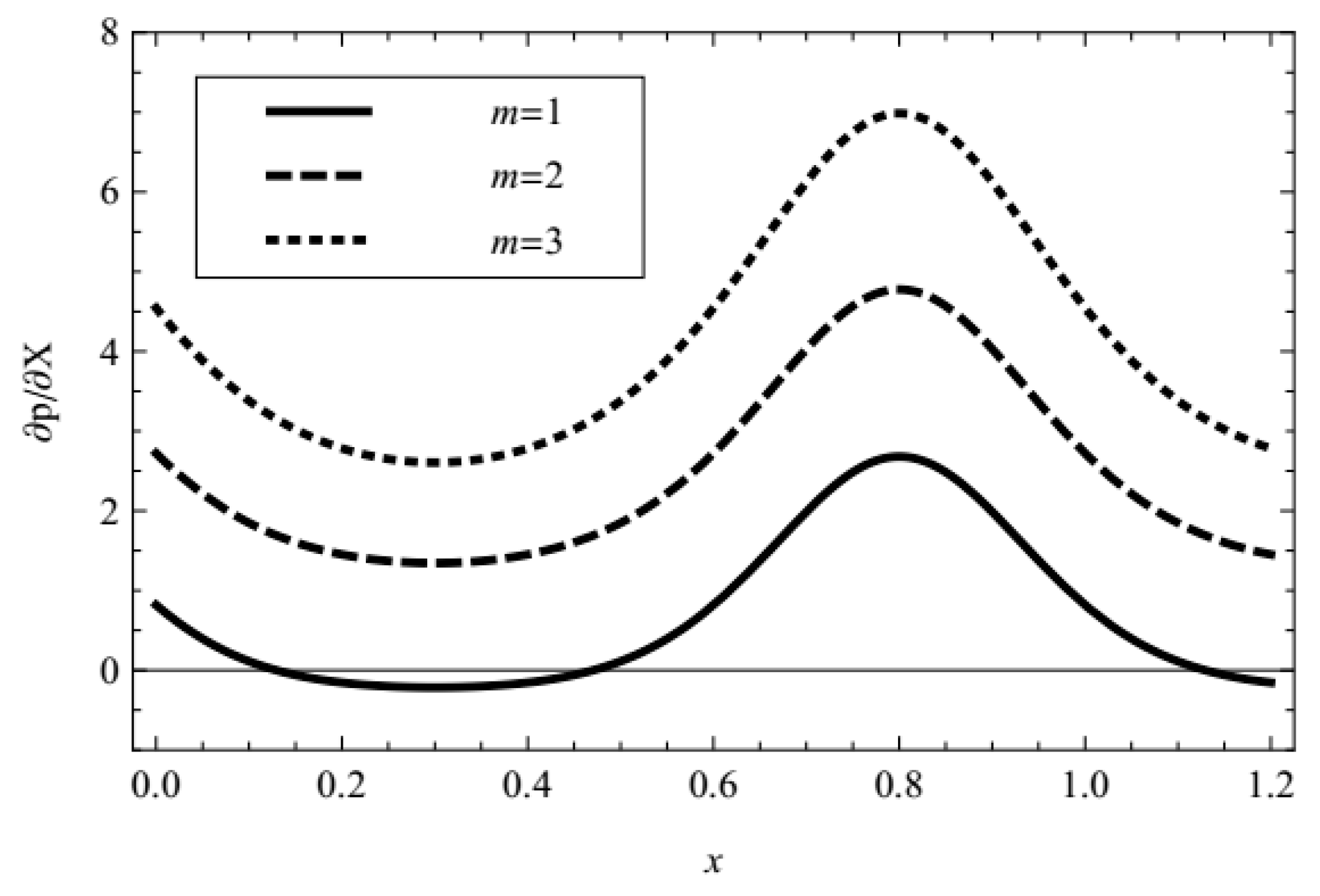
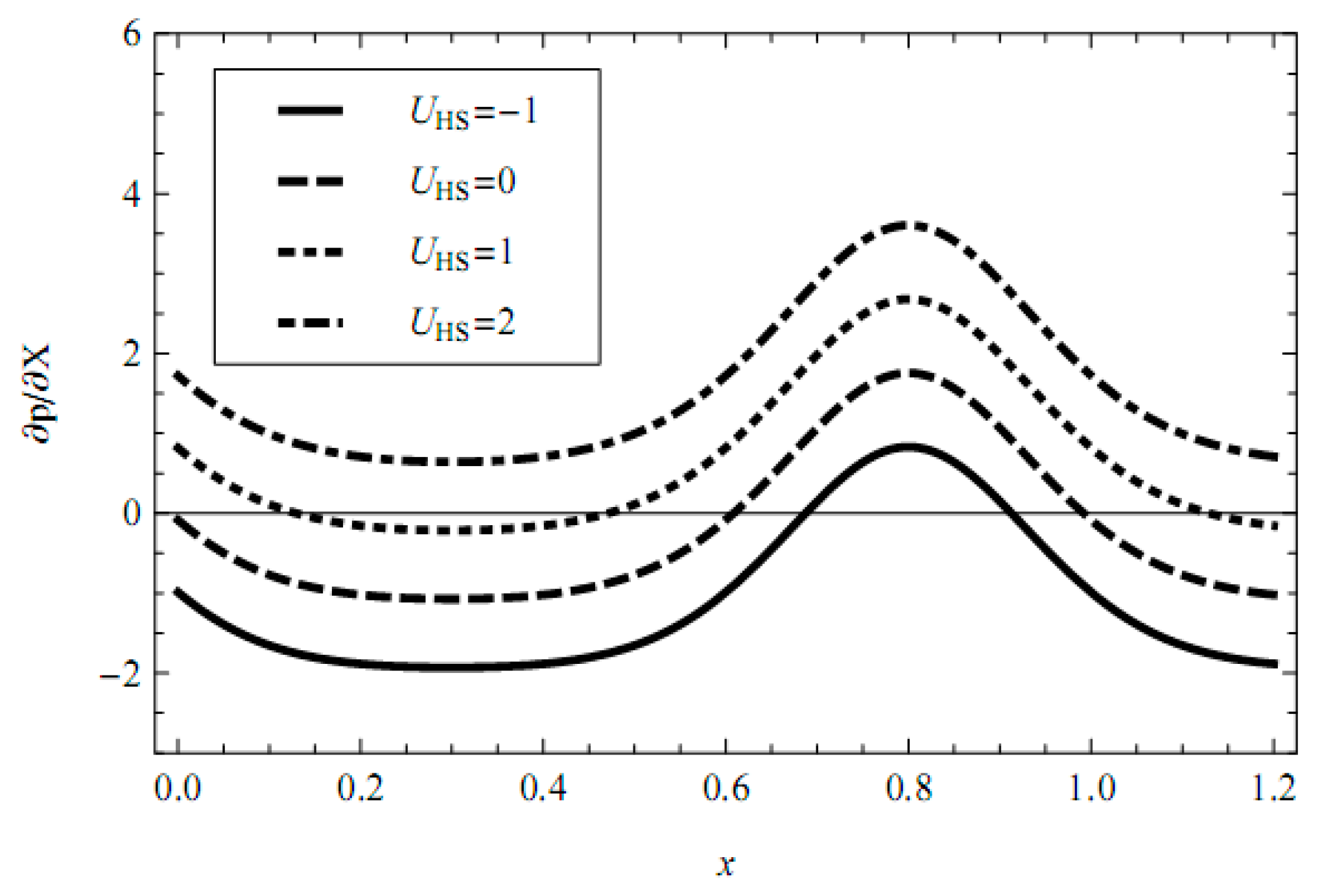
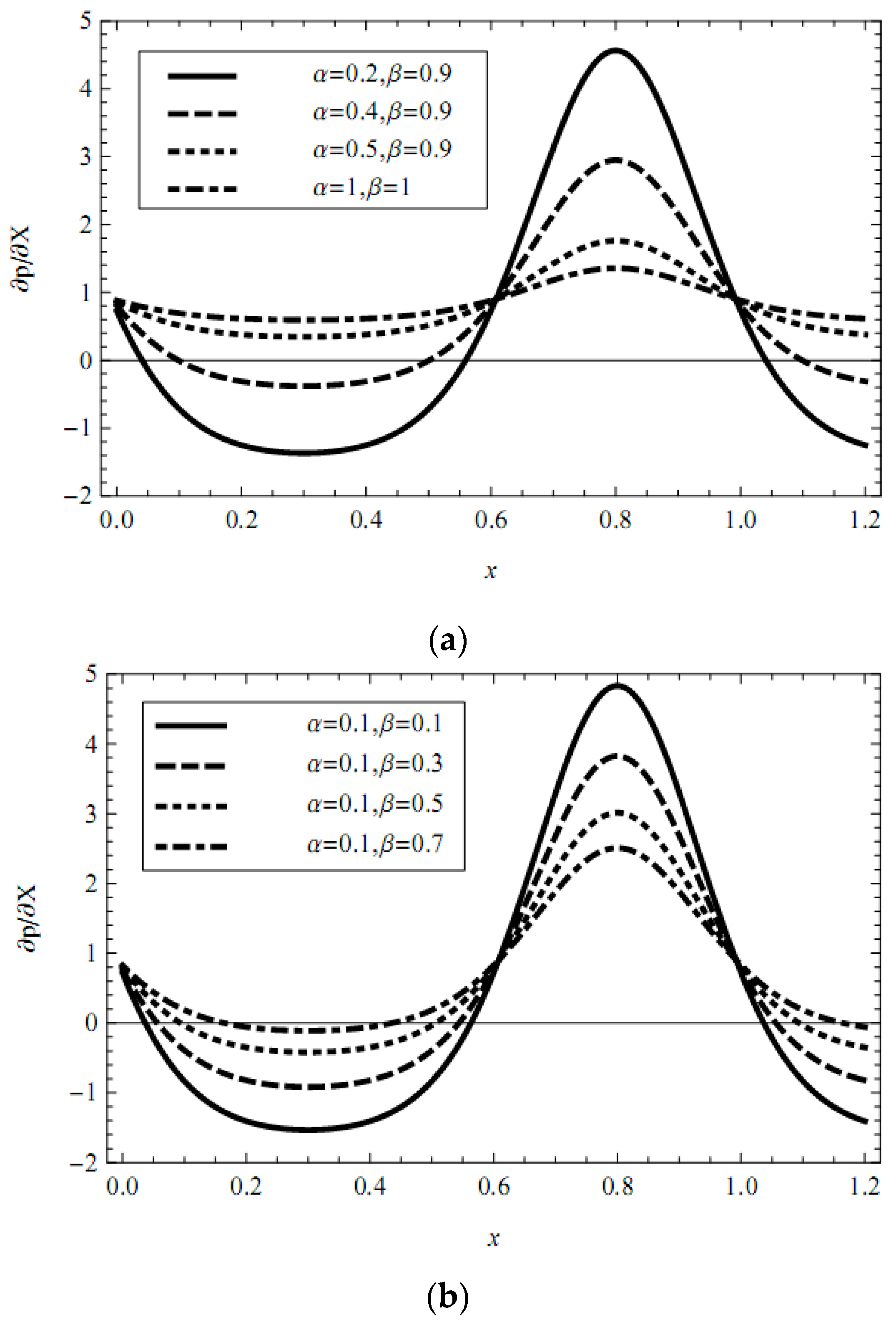
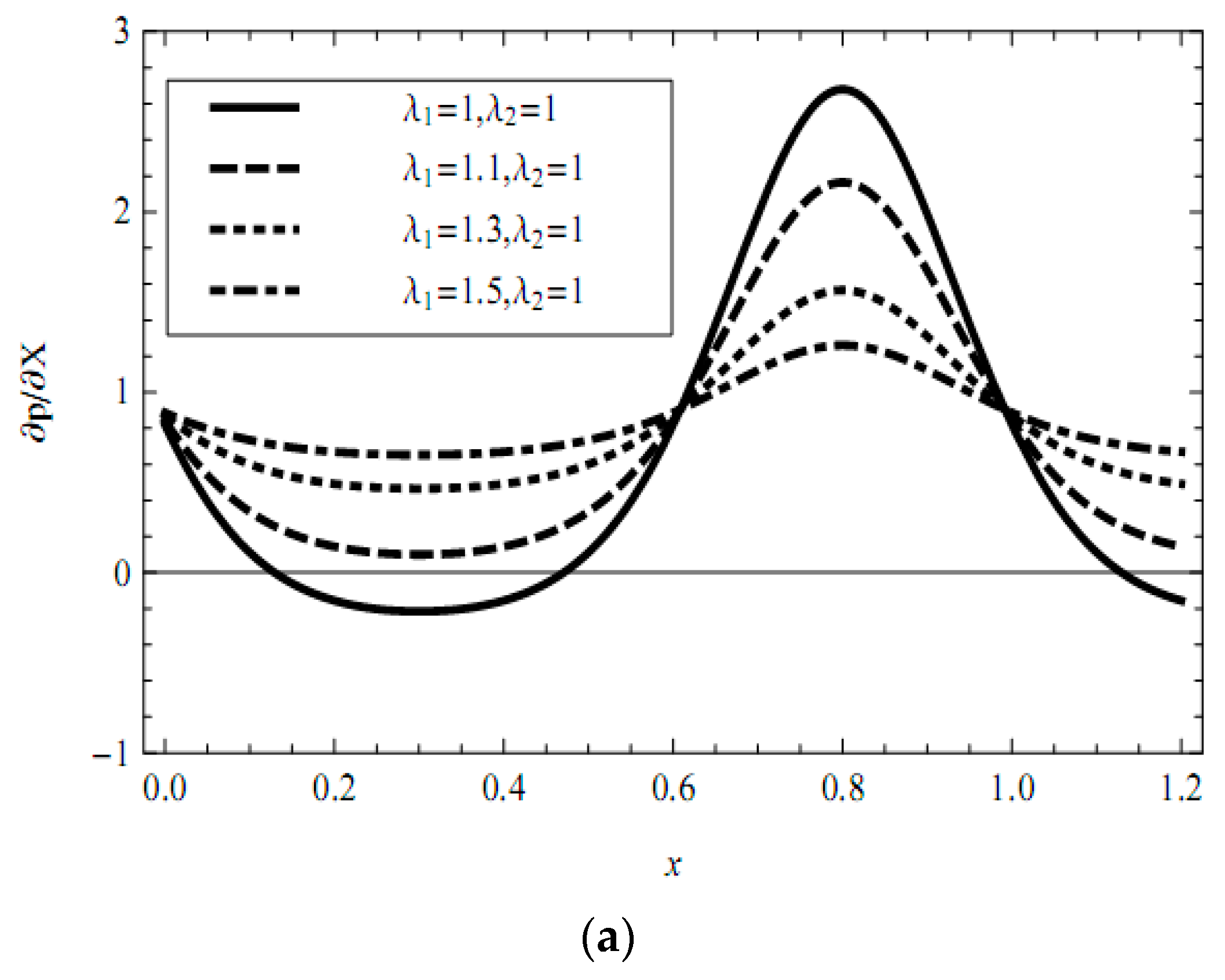
In addition, the influences of pertinent parameters on the flow motion are discussed through graphical illustrations. Firstly, we consider the effects of characteristic thickness of EDL, external electric field, fractional parameters, and viscoelastic parameters on the pressure gradient. Figure 2, Figure 3, Figure 4, Figure 5 and Figure 6 present the axial pressure gradient profiles, i.e., the pressure gradient vs. the axial coordinate along the center line of the channel in one period with fixed time and flow rate. Evidently the pressure gradient profiles are uniform and exhibits periodicity due to the nature of the peristaltic flow, i.e., it is at a minimum at fully-relaxed wall locations and exhibits maximum values at fully-contracted wall locations. In Figure 2, Figure 3, Figure 4, Figure 5 and Figure 6 we find also that, because of the contraction and relaxation of the walls of the channel, there always exists a negative pressure gradient which causes the forward propagation of the trapped bolus.
Figure 2 depicts the pressure gradient for increasing Debye-Hückel parameter (which is inversely proportional to Debye length or characteristic thickness of EDL). It is noticed that the pressure gradient is elevated with the increasing Debye-Hückel parameter, i.e., with decreasing characteristic thickness of EDL, and the decreasing characteristic thickness of EDL can reduce the negative pressure gradient.
The effect of the Helmholtz-Smoluchowski velocity (which is proportional to external electric field) on the pressure gradient is shown in Figure 3. It is observed that, with an increase in the Helmholtz-Smoluchowski velocity, i.e., with an increase in the external electric field there is a consistent enhancement in the pressure gradient, and the increasing external electric field strength can restrain the negative pressure gradient.
In Figure 4a,b, we show the effects of the fractional parameters (α, β) on the pressure gradient. Figure 4a depicts the pressure gradient profiles as α is increased from 0.2 through 0.4 to 0.5 with β fixed at 0.9. The increase in parameter α is observed to reduce the pressure gradient at contracted wall locations, and to enhance the pressure gradient at relaxed wall locations, inversely. Figure 4a also depicts the pressure gradient for classical Jeffreys fluid (α = β = 1). We find that the changes in pressure gradient of the fractional Jeffreys fluid are more significant than that of classical Jeffreys fluid. Figure 4b shows that the pressure gradient decreases with increasing β at contracted wall locations and inversely at relaxed wall locations.
Figure 5a,b illustrates the effects of viscoelastic parameters (relaxation time and retardation time) on the pressure gradient distribution. In Figure 5a, the maximum value of pressure gradient decreases with increasing relaxation time, while the minimum value increases. Inversely, in Figure 5b, the maximum value of pressure gradient enhances with greater value of retardation time, while the minimum reduces. It is concluded that the elasticity of the viscoelastic fluid suppresses the negative pressure gradient because, in general, for the viscoelastic model with greater relaxation time, the fluid is more elastic.
For comparison, the pressure gradient of fractional Jeffreys fluid (FJF), generalized second fluid (GSF), fractional Maxwell fluid (FMF), and Newtonian fluid (NF) are plotted in Figure 6. It is observed that the amplitude of the pressure gradient of fractional Jeffreys fluid falls in between that of generalized second fluid and fractional Maxwell fluid in the same situation.
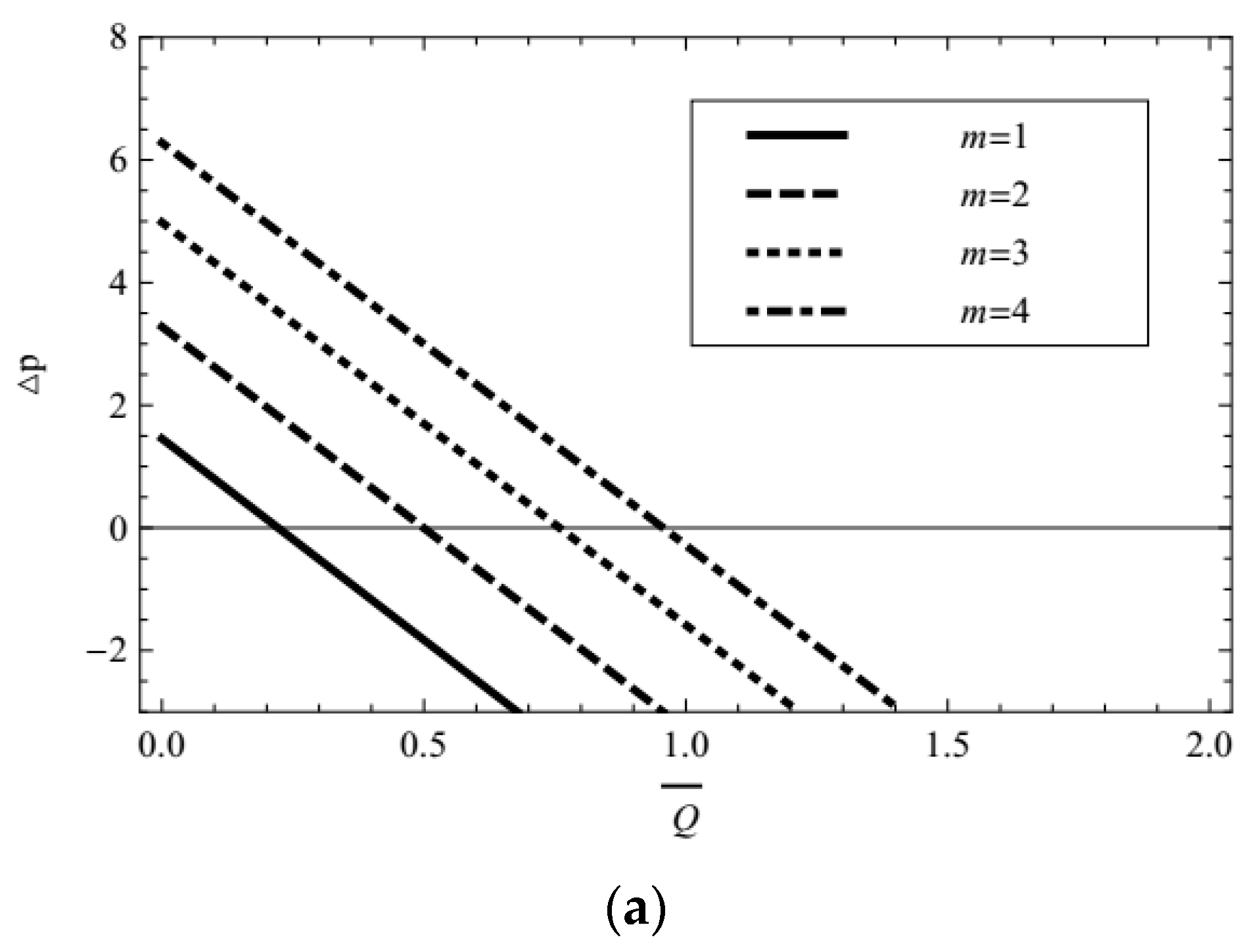
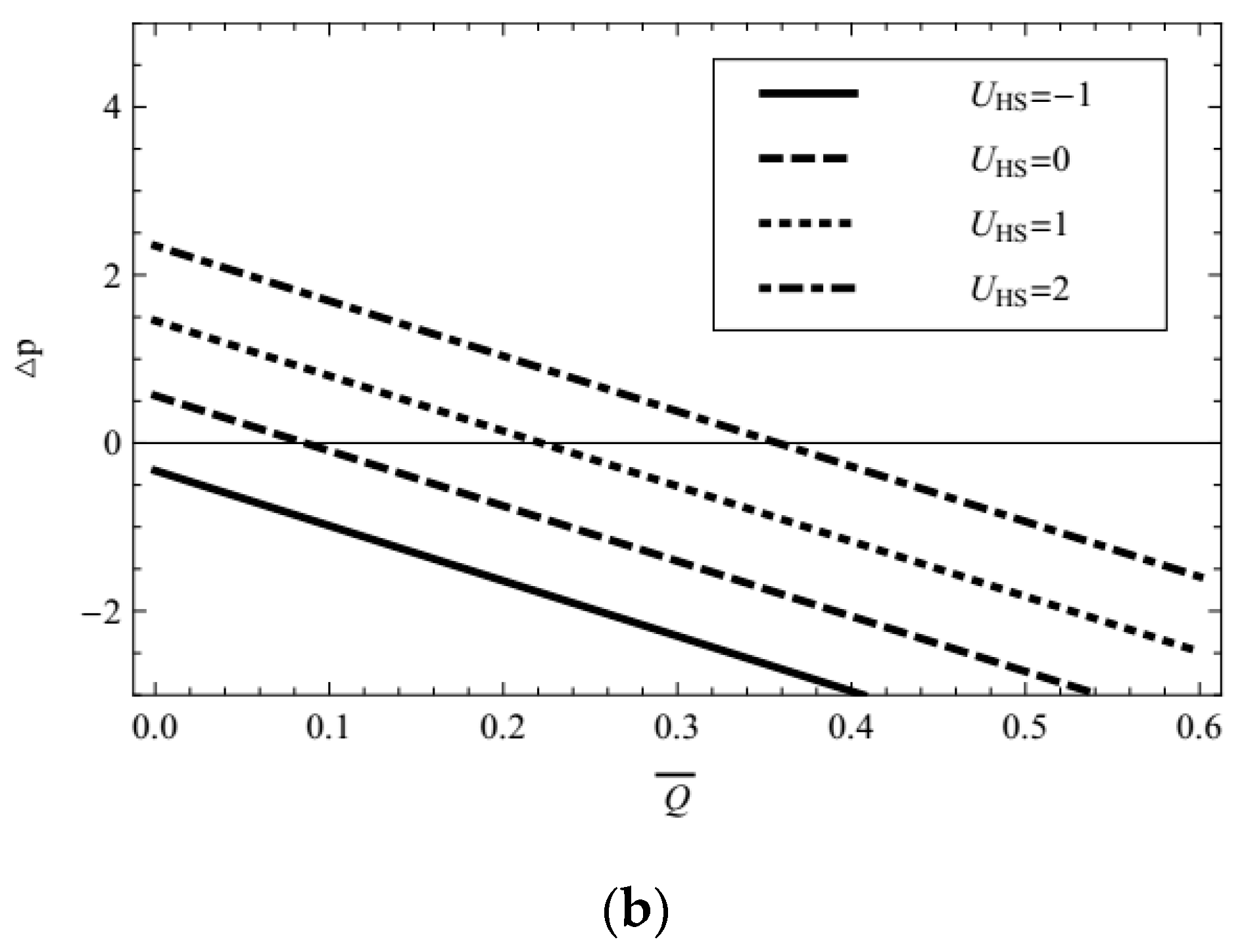
The profile of pressure rise vs. the time averaged volumetric flow rate for different values of Debye-Hückel parameter and Helmholtz-Smoluchowski velocity are given in Figure 7a,b. Obviously the pressure rise is the linear function of the flow rate, and decreases with the greater flow rate. Figure 7a shows that increasing Debye-Hückel parameter, i.e., decreasing characteristic thickness of EDL elevates the pressure rise remarkably. As the Helmholtz-Smoluchowski velocity (i.e., external electric field) increases, Figure 7b illustrates that there is also a consistent elevation in the pressure rise. Especially when UHS = −1, the pressure is always negative for all flow rates.
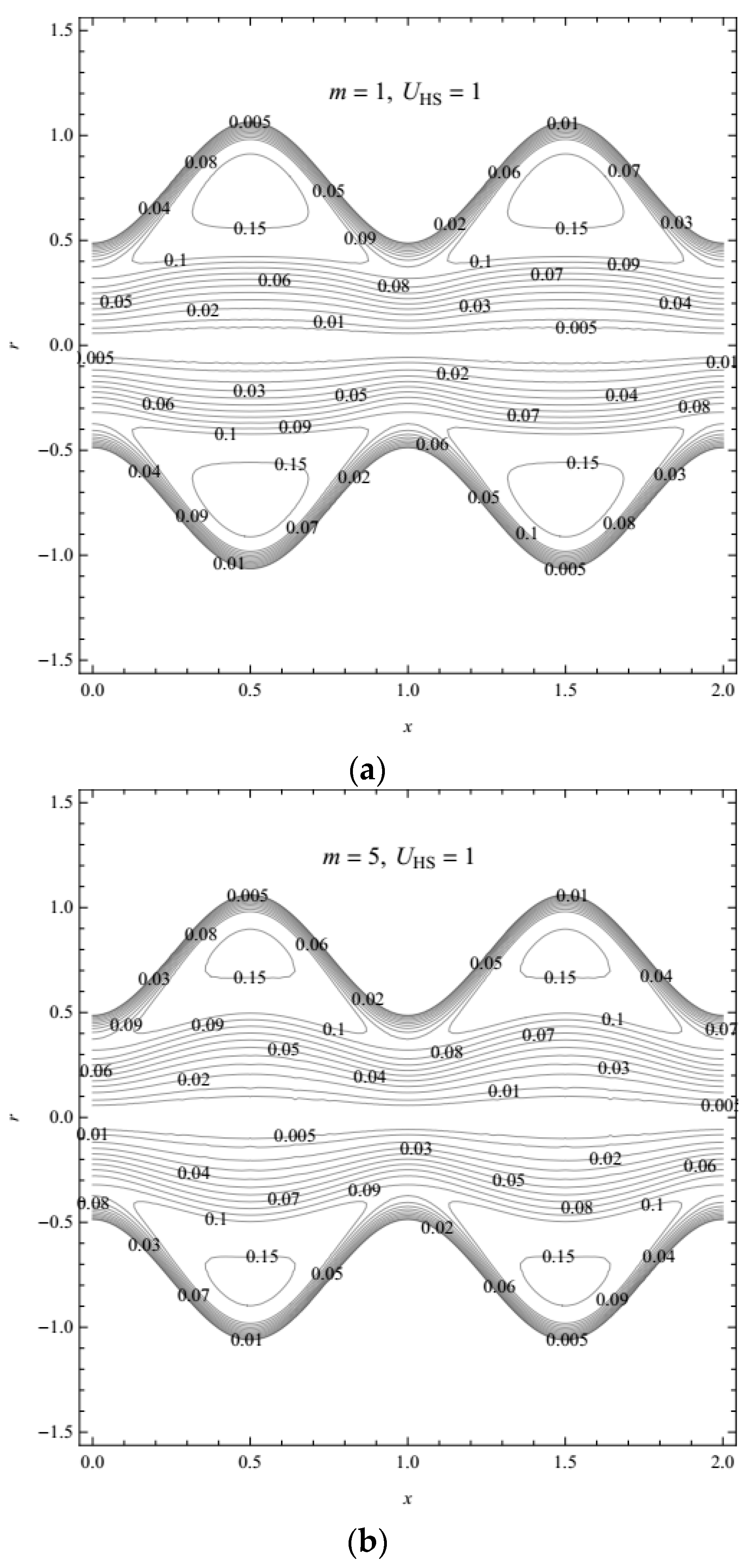
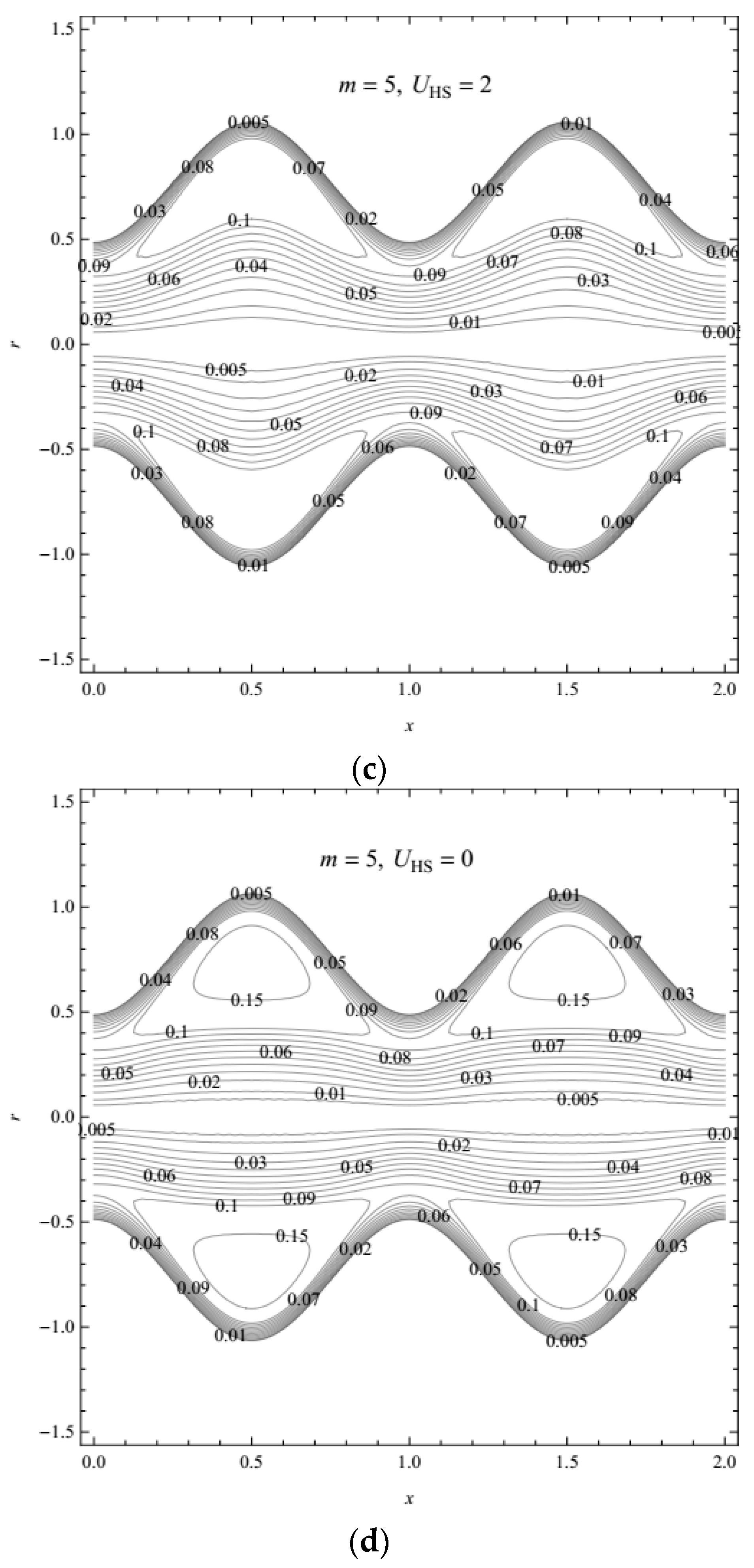
Furthermore, trapping, as an important phenomenon of peristaltic transport, is considered. In Figure 8a–d, we give the stream function profiles (radial coordinates versus axial coordinates) for different values of the Debye-Hückel parameter and Helmholtz-Smoluchowski velocity (with and without an external electric field). In Figure 8a,b, it is evident that with the increasing Debye-Hückel parameter, i.e., the decreasing characteristic thickness of EDL, the range of trapped boluses is reduced. In Figure 8b–d, it is observed that when the external electric field is strong enough, the number of trapped boluses significantly reduces with a larger value of the Helmholtz-Smoluchowski velocity (which is proportional to the external electric field).
5. Conclusions
In this paper, a mathematic model of the electro-osmotic peristaltic flow for fractional Jeffreys fluid through a cylindrical micro-channel is established. Considering the assumptions of long wavelength, low Reynolds number and Debye-Hückel linearization, the analytical solution of pressure gradient, velocity, and streamline function are presented by using integral transform method of fractional operater. The solutions of the corresponding flow for fractional Maxwell fluid, generalized second fluid, and Newtonian fluid are discussed as the special cases. The visualization solutions via Mathematica software have been shown to evaluate the effects of the electro-osmotic parameter (i.e., Debye-Hückel parameter), external electric field, fractional parameters (α, β), and viscoelastic parameters on the peristaltic flow and trapping phenomena. The present computations have shown that:
- The axial pressure gradient is elevated with the increasing Debye-Hückel parameter (i.e., decreasing characteristic thickness of EDL) and the increasing external electric field in all ranges of the axial coordinate. In contracted wall locations, the pressure gradient decreases with the increasing fractional parameter (α, β) and relaxation time, and also with decreasing retardation time. In relaxed wall locations, the converse response is observed and the negative pressure gradient is generated in some cases.
- The pressure rise increases with the increasing Debye-Hückel parameter (i.e., decreasing characteristic thickness of EDL) and the increasing external electric field in all ranges of time-averaged volumetric flow rate. When the pressure rise is fixed, the flow rate is increased with a decrease in the characteristic thickness of EDL and an increase in the external electric field. The influence of the characteristic thickness of EDL on the pressure rise is more remarkable than that of the external electric field.
- The trapped boluses are suppressed with the increasing Debye-Hückel parameter, i.e., a decreasing characteristic thickness of EDL and with a larger value of the Helmholtz-Smoluchowski velocity (which is proportional to the external electric field).
Acknowledgments
This work was supported by National Natural Science Foundation of China (grant Nos. 11402108, 11672163, and 11571157), the Natural Science Foundation of Shandong Province (grant Nos. ZR2015AM011 and BS2015DX012), and Applied Mathematics Enhancement Program of Linyi University.
Author Contributions
X.G. and H.Q. conceived the idea, designed the research, performed the research, analyzed the data and wrote the paper. All authors discussed the results and revised the manuscript.
Conflicts of Interest
The authors declare no conflict of interest.
References
- Sadr, R.; Yoda, M.; Zheng, Z.; Conlisk, A.T. An experimental study of electro-osmotic flow in rectangular microchannels. J. Fluid Mech. 2004, 506, 357–367. [Google Scholar] [CrossRef]
- Santiago, J.G. Electroosmotic flows in microchannels with finite inertial and pressure forces. Anal. Chem. 2001, 73, 2353–2365. [Google Scholar] [CrossRef] [PubMed]
- Yang, C.; Li, D. Analysis of electrokinetic effects on the liquid flow in rectangular microchannels. Colloids Surf. A Physicochem. Eng. Asp. 1998, 143, 339–353. [Google Scholar] [CrossRef]
- Wang, C.Y.; Liu, Y.H.; Chang, C.C. Analytical solution of electro-osmotic flow in a semicircular microchannel. Phys. Fluids 2008, 20, 063105. [Google Scholar] [CrossRef]
- Jian, Y.; Yang, L.; Liu, Q. Time periodic electro-osmotic flow through a microannulus. Phys. Fluids 2010, 22, 1084. [Google Scholar] [CrossRef]
- Hlushkou, D.; Kandhai, D.; Tallarek, U. Coupled lattice-Boltzmann and finite-difference simulation of electroosmosis in microfluidic channels. Int. J. Numer Methods Fluids 2004, 46, 507–532. [Google Scholar] [CrossRef]
- Das, S.; Chakraborty, S. Analytical solutions for velocity, temperature and concentration distribution in electroosmotic microchannel flows of a non-Newtonian bio-fluid. Anal. Chim. Acta 2006, 559, 15–24. [Google Scholar] [CrossRef]
- Chakraborty, S. Electroosmotically driven capillary transport of typical non-Newtonian biofluids in rectangular microchannels. Anal. Chim. Acta 2007, 605, 175–184. [Google Scholar] [CrossRef] [PubMed]
- Zhao, C.; Zholkovskij, E.; Masliyah, J.H.; Yang, C. Analysis of electroosmotic flow of power-law fluids in a slit microchannel. J. Colloid Interface Sci. 2008, 326, 503–510. [Google Scholar] [CrossRef] [PubMed]
- Park, H.M.; Lee, W.M. Effect of viscoelasticity on the flow pattern and the volumetric flow rate in electroosmotic flows through a microchannel. Lab A Chip 2008, 8, 1163–1170. [Google Scholar] [CrossRef] [PubMed]
- Zhao, M.; Wang, S.; Wei, S. Transient electro-osmotic flow of Oldroyd-B fluids in a straight pipe of circular cross section. J. Non-Newton. Fluid Mech. 2013, 201, 135–139. [Google Scholar] [CrossRef]
- Ferrás, L.L.; Afonso, A.M.; Alves, M.A.; Nóbrega, J.M.; Pinho, F.T. Analytical and numerical study of the electro-osmotic annular flow of viscoelastic fluids. J. Colloid Interface Sci. 2014, 420, 152–157. [Google Scholar] [CrossRef] [PubMed] [Green Version]
- Escandón, J.; Jiménez, E.; Hernández, C.; Bautista, O.; Méndez, F. Transient electroosmotic flow of Maxwell fluids in a slit microchannel with asymmetric zeta potentials. Eur. J. Mech. B Fluids 2015, 53, 180–189. [Google Scholar] [CrossRef]
- Latham, T.W. Fluid Motions in a Peristaltic Pump; Massachusetts Institute of Technology: Cambridge, MA, USA, 1966. [Google Scholar]
- Yin, F.; Fung, Y.C. Peristaltic Waves in Circular Cylindrical Tubes. J. Appl. Mech. 1969, 36, 579–587. [Google Scholar] [CrossRef]
- Weinberg, S.L.; Eckstein, E.C.; Shapiro, A.H. An experimental study of peristaltic pumping. J. Fluid Mech. 1971, 49, 461–479. [Google Scholar] [CrossRef]
- Srivastava, L.M. Peristaltic transport of a couple-stress fluid. Rheol. Acta 1986, 25, 638–641. [Google Scholar] [CrossRef]
- Siddiqui, A.M.; Schwarz, W.H. Peristaltic flow of a second-order fluid in tubes. J. Non-Newton. Fluid Mechan. 1994, 53, 257–284. [Google Scholar] [CrossRef]
- Hayat, T.; Alvi, N.; Ali, N. Peristaltic mechanism of a Maxwell fluid in an asymmetric channel. Nonlinear Anal. Real World Appl. 2008, 9, 1474–1490. [Google Scholar] [CrossRef]
- Kothandapani, M.; Srinivas, S. Peristaltic transport of a Jeffrey fluid under the effect of magnetic field in an asymmetric channel. Int. J. Non-Linear Mech. 2008, 43, 915–924. [Google Scholar] [CrossRef]
- Srinivas, S.; Gayathri, R. Peristaltic transport of a Newtonian fluid in a vertical asymmetric channel with heat transfer and porous medium. Appl. Math. Comput. 2009, 215, 185–196. [Google Scholar] [CrossRef]
- Hayat, T.; Javed, M.; Ali, N. MHD Peristaltic Transport of a Jeffery Fluid in a Channel with Compliant Walls and Porous Space. Transp. Porous Media 2008, 74, 259–274. [Google Scholar] [CrossRef]
- Hayat, T.; Rafiq, M.; Ahmad, B. Soret and Dufour Effects on MHD Peristaltic Flow of Jeffrey Fluid in a Rotating System with Porous Medium. PLoS ONE 2016, 11, e0145525. [Google Scholar] [CrossRef] [PubMed]
- Singh, J.; Rathee, R. Analysis of non-Newtonian blood flow through stenosed vessel in porous medium under the effect of magnetic field. Int. J. Phys. Sci. 2011, 6, 2497–2506. [Google Scholar]
- Zeeshan, A.; Ellahi, R. Series solutions of nonlinear partial differential equations with slip boundary conditions for non-Newtonian MHD fluid in porous space. Appl. Math. Inf. Sci. 2013, 7, 253–261. [Google Scholar] [CrossRef]
- Bhatti, M.M.; Riaz, A.; Ellahi, R.; Sheikholeslami, M. Effects of magnetohydrodynamics on peristaltic flow of Jeffrey fluid in a rectangular duct through a porous medium. J. Porous Media 2014, 17, 143–157. [Google Scholar]
- Rashidi, M.M.; Bhatti, M.M.; Abbas, M.A.; Ali, M.E.S. Entropy Generation on MHD Blood Flow of Nanofluid Due to Peristaltic Waves. Entropy 2016, 18, 117. [Google Scholar] [CrossRef]
- Bandopadhyay, A.; Tripathi, D.; Chakraborty, S. Electroosmosis-modulated peristaltic transport in microfluidic channels. Phys. Fluids 2016, 28, 052002. [Google Scholar] [CrossRef]
- Goswami, P.; Chakraborty, J.; Bandopadhyay, A.; Chakraborty, S. Electrokinetically modulated peristaltic transport of power-law fluids. Microvasc. Res. 2016, 103, 41–54. [Google Scholar] [CrossRef] [PubMed]
- Tripathi, D.; Yadav, A.; Bég, O.A. Electro-osmotic flow of couple stress fluids in a micro-channel propagated by peristalsis. Eur. Phys. J. Plus 2017, 132, 173. [Google Scholar] [CrossRef]
- Tripathi, D.; Bhushan, S.; Bég, O.A. Analytical study of electro-osmosis modulated capillary peristaltic hemodynamics. J. Mech. Med. Biol. 2017, 17, 1750052. [Google Scholar] [CrossRef]
- Song, D.Y.; Jiang, T.Q. Study on the constitutive equation with fractional derivative for the viscoelastic fluids—Modified Jeffreys model and its application. Rheol. Acta 1998, 37, 512–517. [Google Scholar] [CrossRef]
- Xu, M.; Tan, W. Intermediate processes and critical phenomena: Theory, method and progress of fractional operators and their applications to modern mechanics. Sci. China Phys. Mech. Astron. 2006, 49, 257–272. [Google Scholar] [CrossRef]
- Tan, W.; Masuoka, T. Stokes’ first problem for a second grade fluid in a porous half-space with heated boundary. Int. J. Non-Linear Mech. 2005, 40, 515–522. [Google Scholar] [CrossRef]
- Guo, X.; Fu, Z. An initial and boundary value problem of fractional Jeffreys’ fluid in a porous half space. Comput. Math. Appl. 2015, in press. [Google Scholar] [CrossRef]
- Tripathi, D.; Pandey, S.K.; Das, S. Peristaltic flow of viscoelastic fluid with fractional Maxwell model through a channel. Appl. Math. Comput. 2010, 215, 3645–3654. [Google Scholar] [CrossRef]
- Tripathi, D.; Bég, O.A.; Curiel-Sosa, J.L. Homotopy semi-numerical simulation of peristaltic flow of generalised Oldroyd-B fluids with slip effects. Comput. Methods Biomech. Biomed. Eng. 2014, 17, 433–442. [Google Scholar] [CrossRef] [PubMed]
- Jamil, M.; Khan, A.N.; Shahid, N. Fractional magnetohydrodynamics Oldroyd-B fluid over an oscillating plate. Therm. Sci. 2013, 17, 997–1011. [Google Scholar] [CrossRef]
- Hameed, M.; Khan, A.A.; Ellahi, R.; Raza, M. Study of magnetic and heat transfer on the peristaltic transport of a fractional second grade fluid in a vertical tube. Eng. Sci. Technol. Int. J. 2015, 37, 496–502. [Google Scholar] [CrossRef]
- Jiang, Y.; Qi, H.; Xu, H.; Jiang, X. Transient electroosmotic slip flow of fractional Oldroyd-B fluids. Microfluid. Nanofluidics 2017, 21, 7. [Google Scholar] [CrossRef]
- Wang, X.; Qi, H.; Yu, B.; Xiong, Z.; Xu, H. Analytical and numerical study of electroosmotic slip flows of fractional second grade fluids. Commun. Nonlinear Sci. Numer. Simul. 2017, 50, 77–87. [Google Scholar] [CrossRef]
- Tan, Z.; Qi, H.; Jiang, X.Y. Electroosmotic flow of Eyring fluid in slit microchannel with slip boundary condition. Appl. Math. Mech. 2014, 35, 689–696. [Google Scholar] [CrossRef]
- Wang, S.; Zhao, M. Analytical solution of the transient electro-osmotic flow of a generalized fractional Maxwell fluid in a straight pipe with a circular cross-section. Eur. J. Mech. B Fluids 2015, 54, 82–86. [Google Scholar] [CrossRef]
- Hayat, T.; Ali, N.; Asghar, S. An analysis of peristaltic transport for flow of a Jeffrey fluid. Acta Mech. 2007, 193, 101–112. [Google Scholar] [CrossRef]
- Podlubny, I. Fractional Differential Equations; Academic Press: San Diego, CA, USA, 1998. [Google Scholar]
Figure 1.
Geometry of the problem.
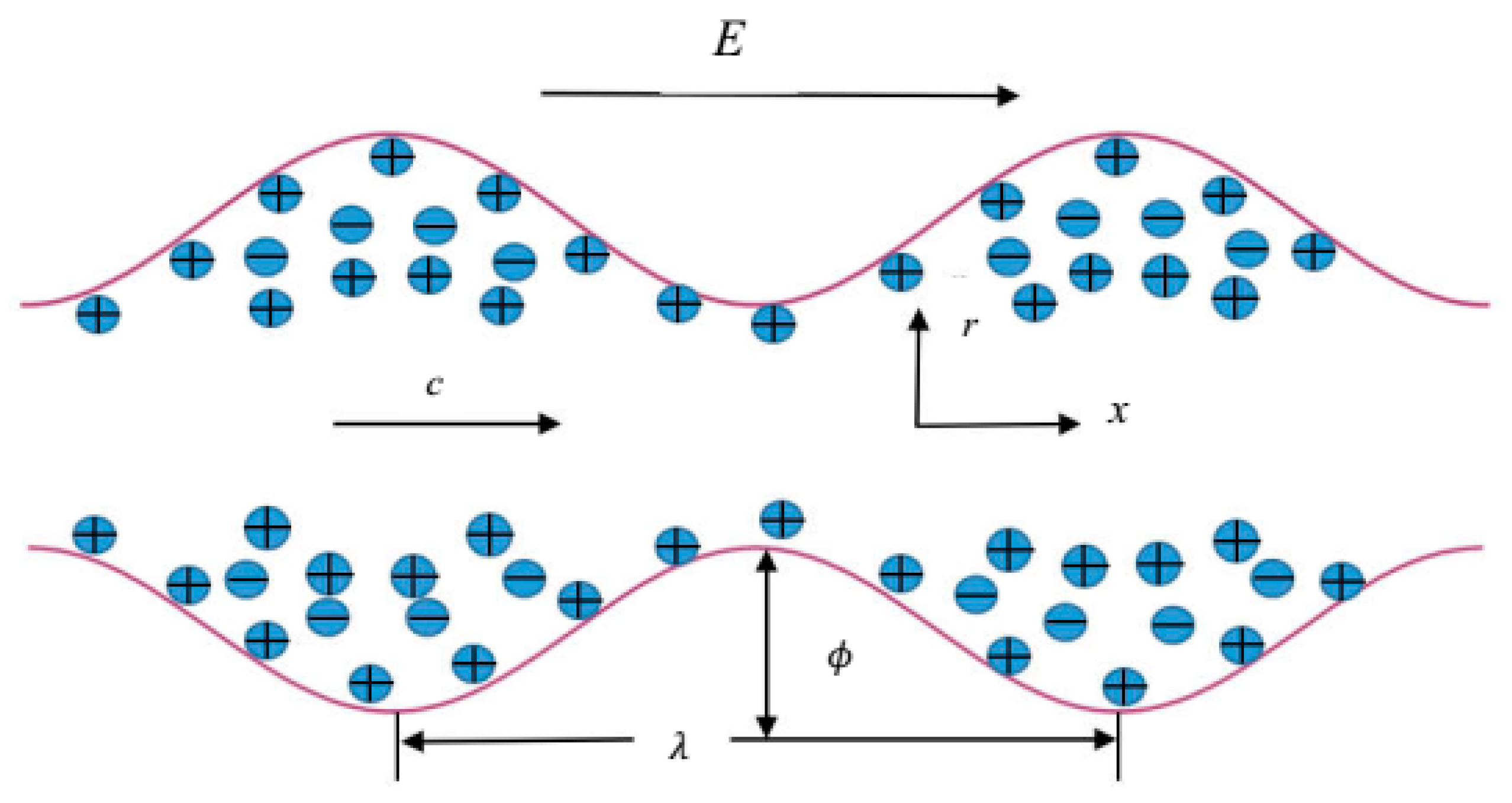
Figure 2.
Profiles of the pressure gradient for various values of m with fixed α = 0.4, β = 0.6, λ1 = 1, λ2 = 1, = 1, = 0.3, = 0.1, t = 0.8.
Figure 2.
Profiles of the pressure gradient for various values of m with fixed α = 0.4, β = 0.6, λ1 = 1, λ2 = 1, = 1, = 0.3, = 0.1, t = 0.8.

Figure 3.
Profiles of the pressure gradient for various values of with fixed α = 0.4, β = 0.6, λ1 = 1, λ2 = 1, m = 1, = 0.3, = 0.1, t = 0.8.
Figure 3.
Profiles of the pressure gradient for various values of with fixed α = 0.4, β = 0.6, λ1 = 1, λ2 = 1, m = 1, = 0.3, = 0.1, t = 0.8.

Figure 4.
Profiles of the pressure gradient for various values of fractional operator parameter (a) α and (b) β with fixed λ1 = 1, λ2 = 1, m = 1, = 0.3, = 1, = 0.1, t = 0.8.
Figure 4.
Profiles of the pressure gradient for various values of fractional operator parameter (a) α and (b) β with fixed λ1 = 1, λ2 = 1, m = 1, = 0.3, = 1, = 0.1, t = 0.8.

Figure 5.
Profiles of the pressure gradient for various values of material parameter (a) λ1 and (b) λ2 with fixed α = 0.4, β = 0.6, m = 1, = 0.3, = 1, = 0.1, t = 0.8.
Figure 5.
Profiles of the pressure gradient for various values of material parameter (a) λ1 and (b) λ2 with fixed α = 0.4, β = 0.6, m = 1, = 0.3, = 1, = 0.1, t = 0.8.

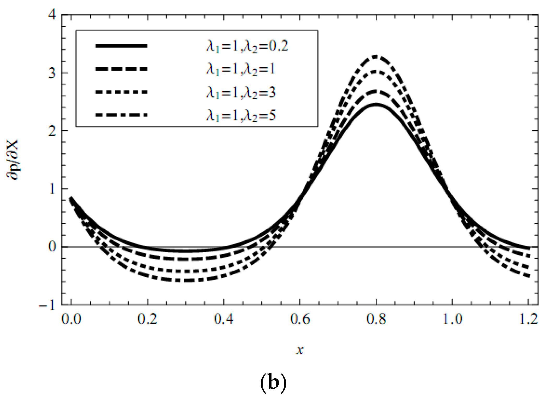
Figure 6.
Profiles of the pressure gradient for fractional Jeffreys fluid (FJF) (α = 0.4, β = 0.6, λ1 = 1, λ2 = 1), generalized second fluid (GSF) (α = 0, β = 0.6, λ1 → 0, λ2 = 1), fractional Maxwell fluid (FMF) (α = 0.4, β = 0, λ1 = 1, λ2 → 0), and Newtonian fluid (NF), with fixed m = 1, = 0.3, = 1, = 0.1, t = 0.8.
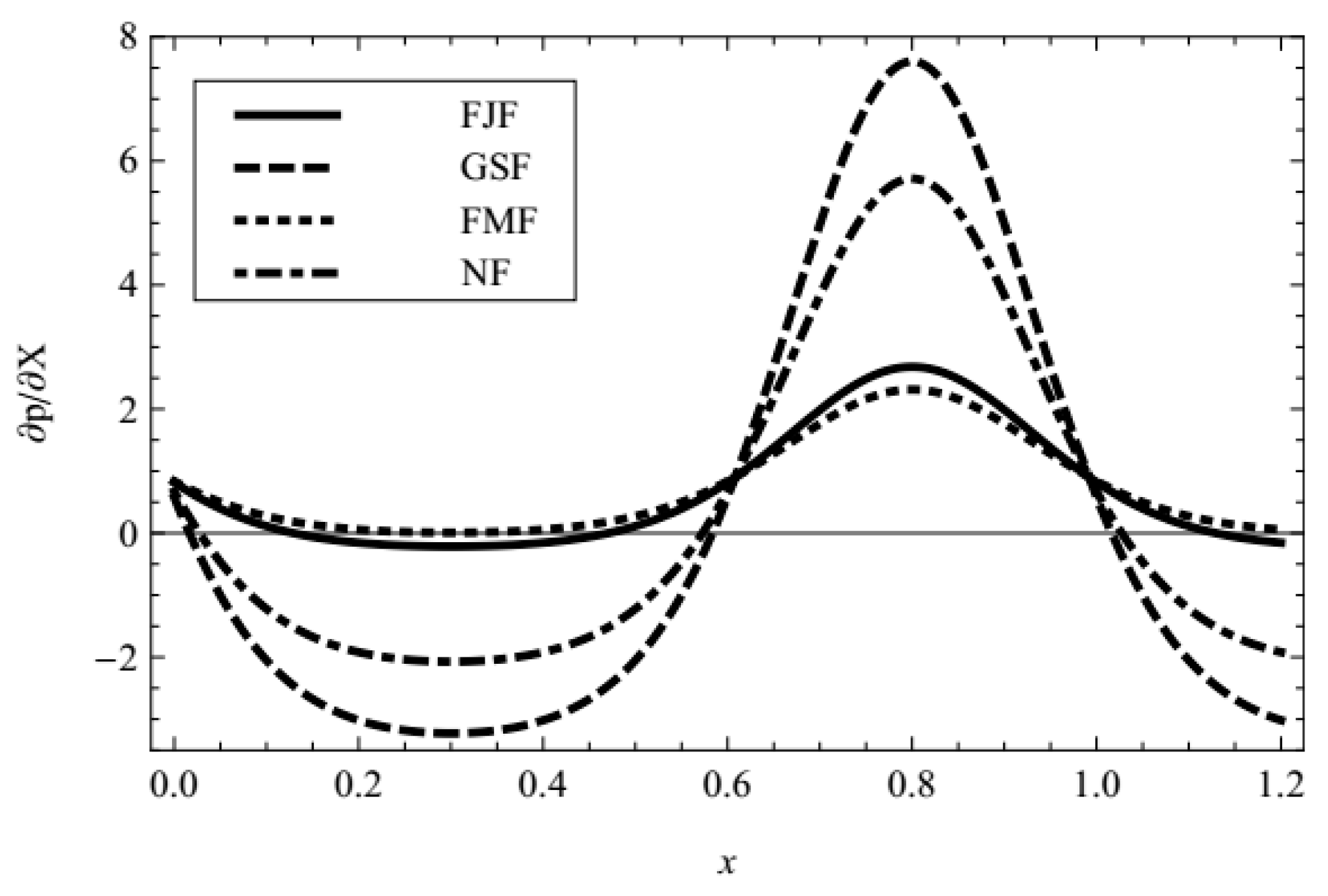
Figure 7.
Profiles of pressure rise vs. time averaged volumetric flow rate for (a) = 1 (b) m = 1, with fixed α = 0.4, β = 0.6, λ1 = 1, λ2 = 1, = 0.3, t = 0.8.
Figure 7.
Profiles of pressure rise vs. time averaged volumetric flow rate for (a) = 1 (b) m = 1, with fixed α = 0.4, β = 0.6, λ1 = 1, λ2 = 1, = 0.3, t = 0.8.


Figure 8.
Profiles of the stream function for different values of m and : (a) m = 1, = 1; (b) m = 5, = 1; (c) m = 5, = 2; (d) m = 5, = 0 with fixed α = 0.4, β = 0.6, λ1 = 1, λ2 = 1, = 0.6, t = 0.8.
Figure 8.
Profiles of the stream function for different values of m and : (a) m = 1, = 1; (b) m = 5, = 1; (c) m = 5, = 2; (d) m = 5, = 0 with fixed α = 0.4, β = 0.6, λ1 = 1, λ2 = 1, = 0.6, t = 0.8.
© 2017 by the authors. Licensee MDPI, Basel, Switzerland. This article is an open access article distributed under the terms and conditions of the Creative Commons Attribution (CC BY) license (http://creativecommons.org/licenses/by/4.0/).
Share and Cite
MDPI and ACS Style
Guo, X.; Qi, H. Analytical Solution of Electro-Osmotic Peristalsis of Fractional Jeffreys Fluid in a Micro-Channel. Micromachines 2017, 8, 341. https://doi.org/10.3390/mi8120341
AMA Style
Guo X, Qi H. Analytical Solution of Electro-Osmotic Peristalsis of Fractional Jeffreys Fluid in a Micro-Channel. Micromachines. 2017; 8(12):341. https://doi.org/10.3390/mi8120341
Chicago/Turabian StyleGuo, Xiaoyi, and Haitao Qi. 2017. "Analytical Solution of Electro-Osmotic Peristalsis of Fractional Jeffreys Fluid in a Micro-Channel" Micromachines 8, no. 12: 341. https://doi.org/10.3390/mi8120341
Note that from the first issue of 2016, this journal uses article numbers instead of page numbers. See further details here.