
Comprehensive Calibration of Strap-Down Tri-Axis Accelerometer Unit


Abstract
:1. Introduction
- (1)
- SINS: strap-down inertial navigation system;
- (2)
- IMU: inertial measurement unit;
- (3)
- MIMU: MEMS inertial measurement unit.
2. Calibration Model
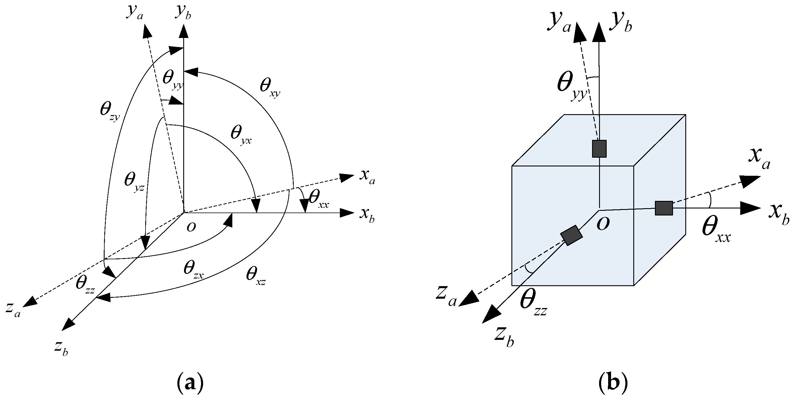
- (1)
- Body coordinate frame (b-frame): its origin Ob is the center of IMU, three orthogonal axials are represented as xb, yb and zb, respectively, and (rx ry rz) is the distance between position of the accelerometer and origin O, respectively.
- (2)
- Sensitive axis coordinate frame (a-frame): xa, ya and za represent a three-coordinate axis in an a-frame.
- (3)
- Navigation coordinate system (n-frame): its origin O is at the center of the gravity vector.
2.1. Calibration Model of Static Error
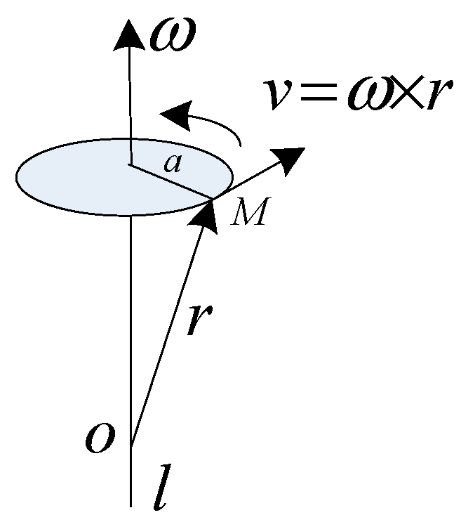
2.2. Calibration Model of Dynamic Error
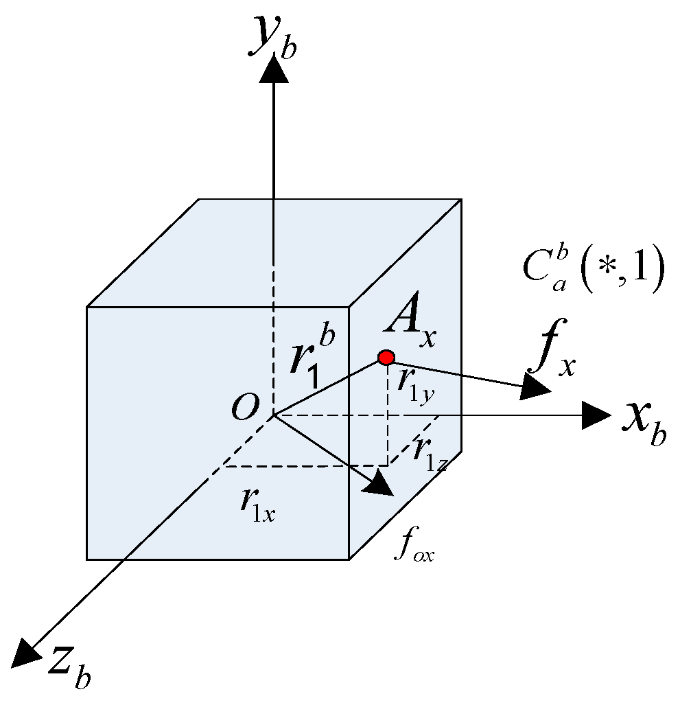
2.3. Identification of Lever Arm
3. Experiments
3.1. Static Calibration Experiment
- (1)
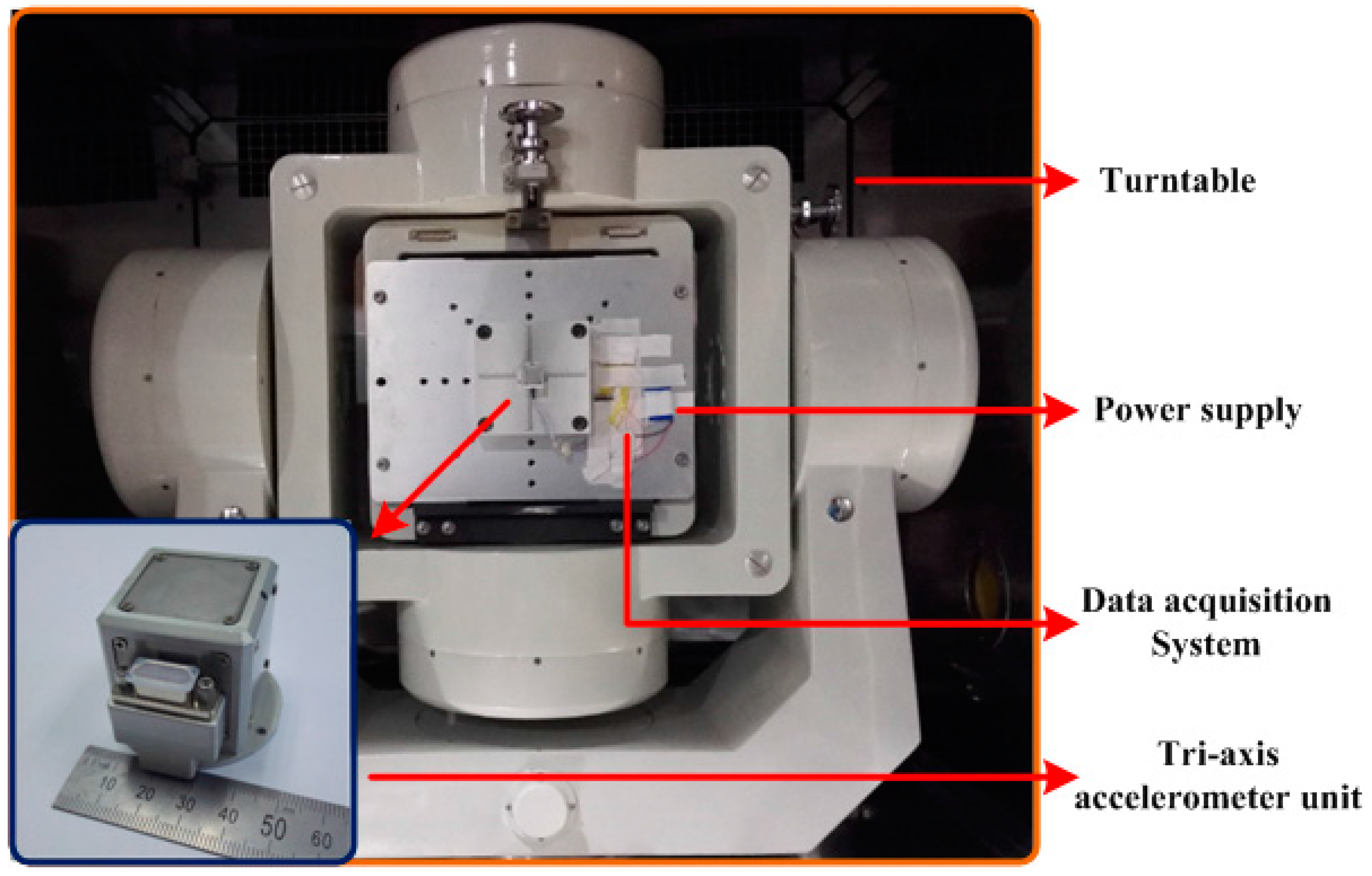
- MIMU, which linked with a real-time acquisition system to collect data, is fixed on the multi-function tri-axial position rate turntable. x-axis upward, y-axis and z-axis point to south and east directions, respectively.
- (2)
- By setting the turntable position, make accelerometer x ideal axis at position ±1 g and collect the output data for a minute at each position.
- (3)
- Turntable is set to make the accelerometers y-axis and z-axis in position ±1 g. Collect the output data for a minute at each position.
- (4)
- According to static parameters calibration model Equation (6), the least squares fitting results can be obtained by using Matlab (version 7.8.0 (R2009a), MathWorks, Natick, MA, USA), which are actual installation angle, zero bias and scale factors of tri-axial accelerometers, respectively.
3.2. Dynamic Calibration Experiment
- (1)
- Fix the MIMU on the turntable, set up the turntable to the x-axis in the vertical position steady for two minutes.
- (2)
- Power on the acquisition system and collect one-minute stationary data. Then, set the turntable rate to rotate in an invariable angular rate ω0 = 100°/s, 150°/s, and 200°/s around the x-axis and collect one minute of data after becoming stable.
- (3)
- Set the turntable to the y-axis and z-axis on the upright position, repeat the first step and record the output of tri-axial accelerometer timely.
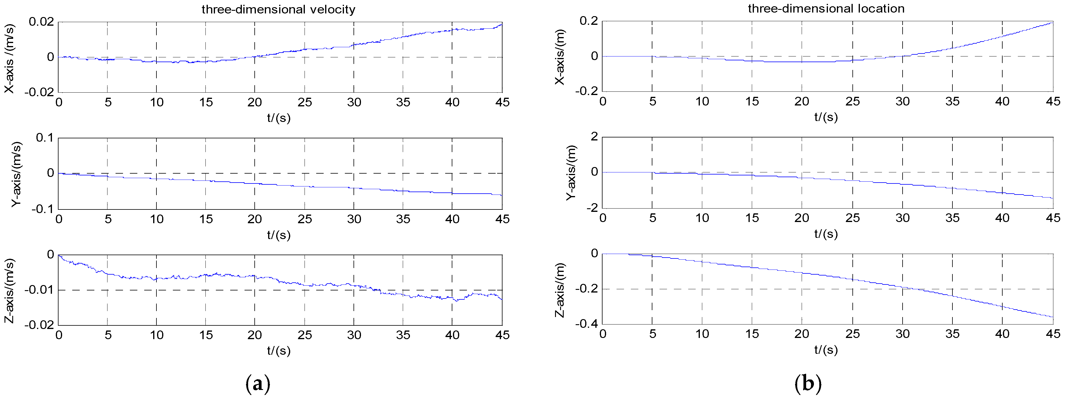
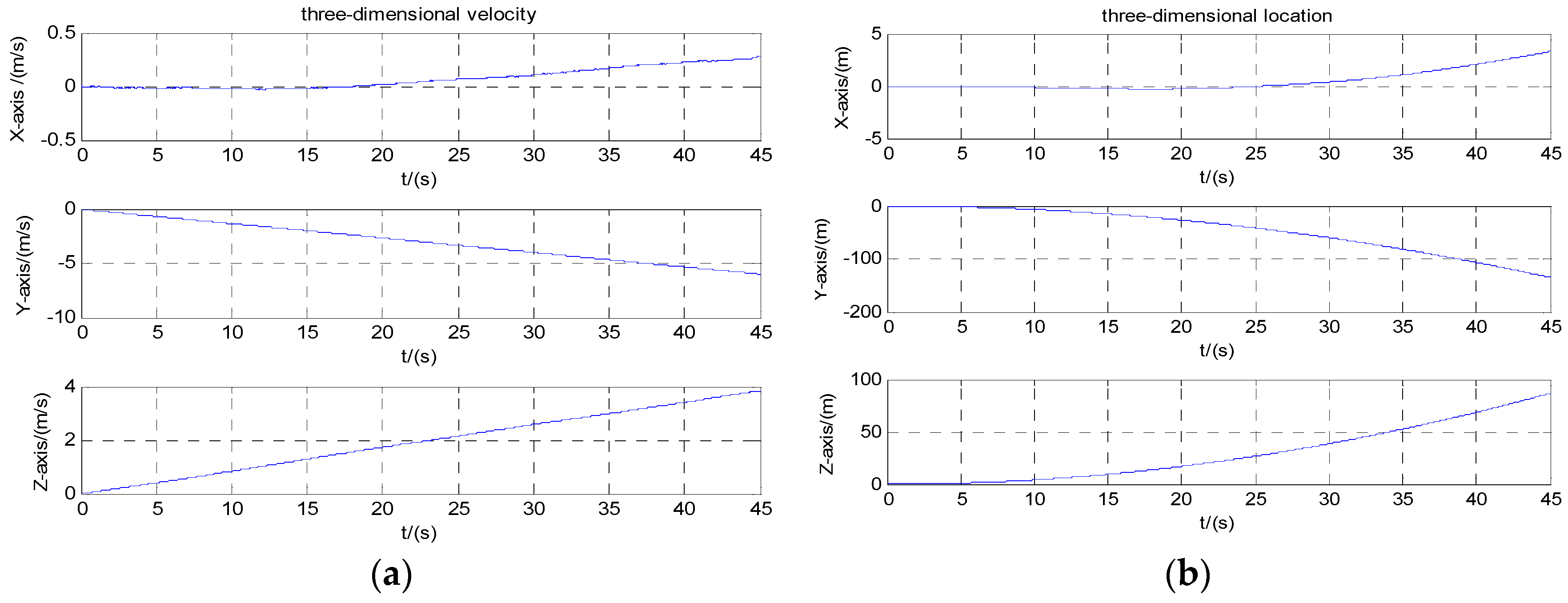
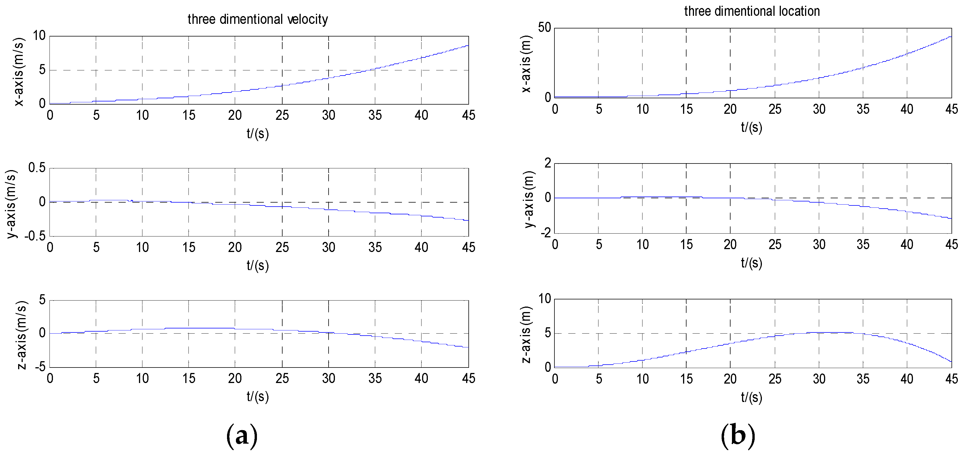
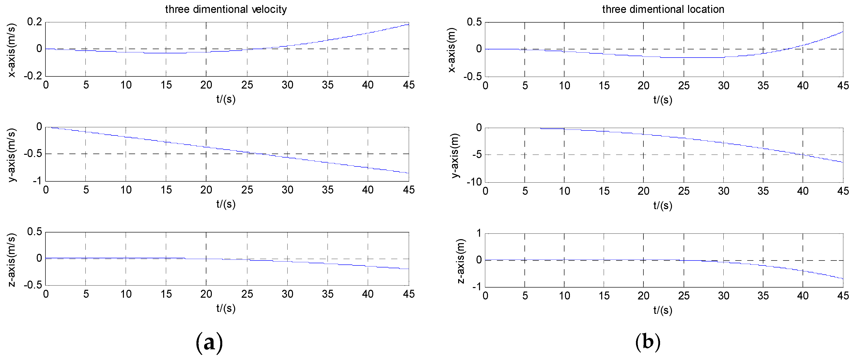
3.3. Ground Verification Experiment
4. Result/Discussion
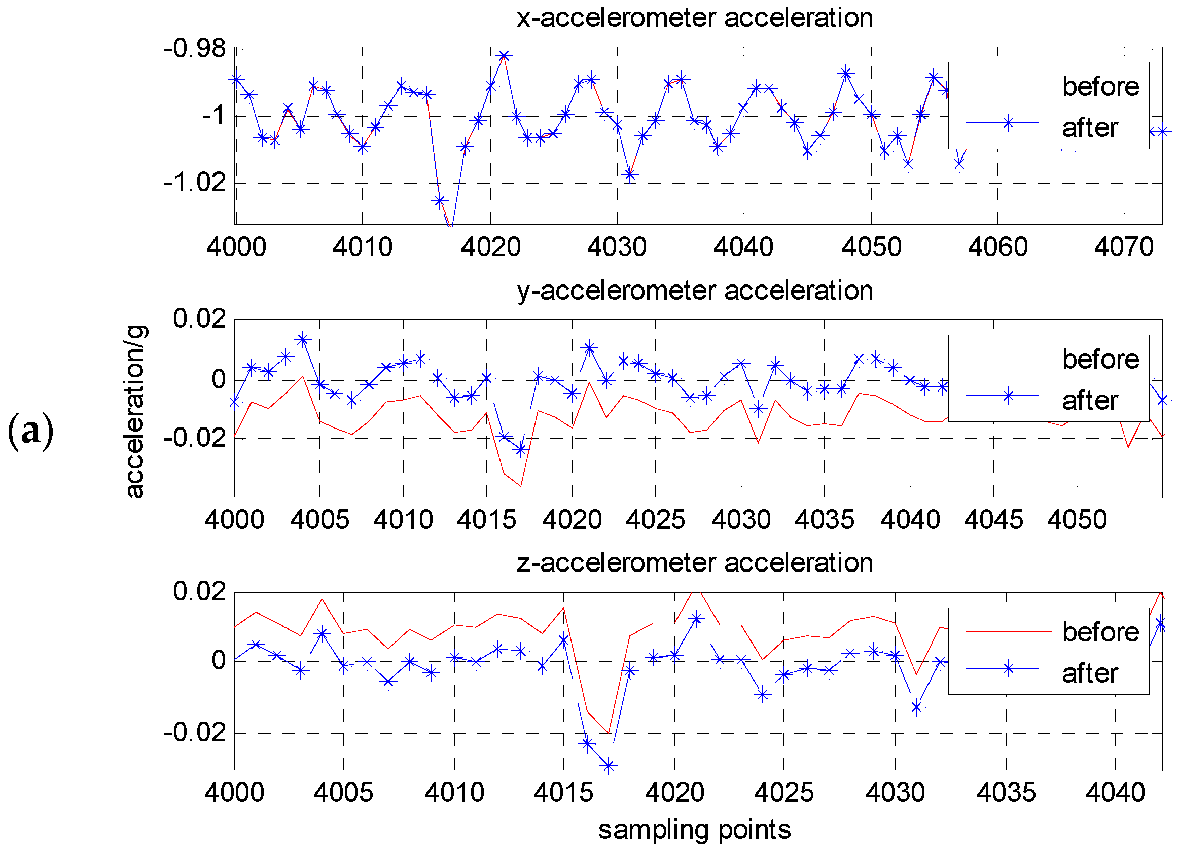
4.1. Static Calibration Result and Discussion
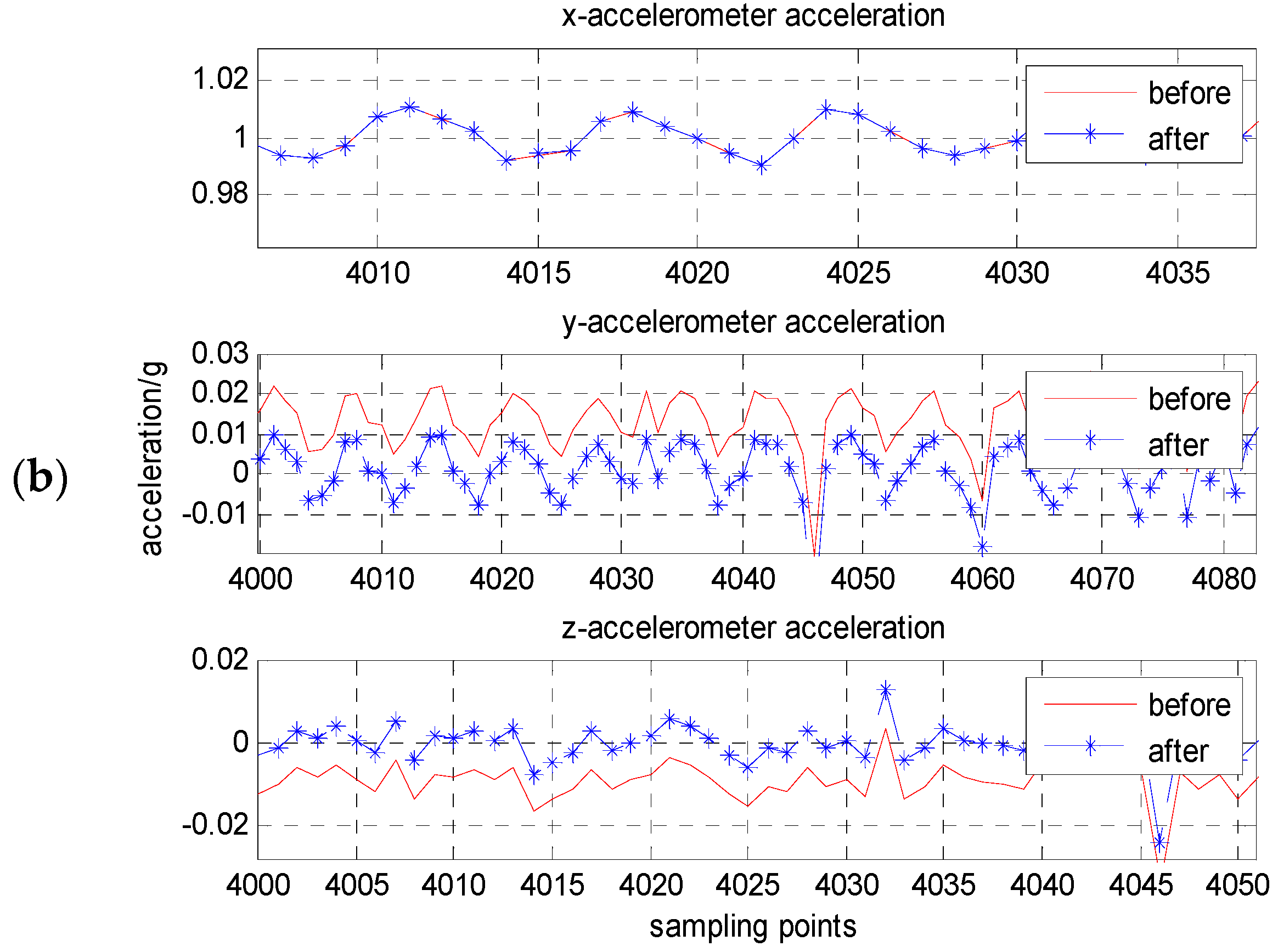
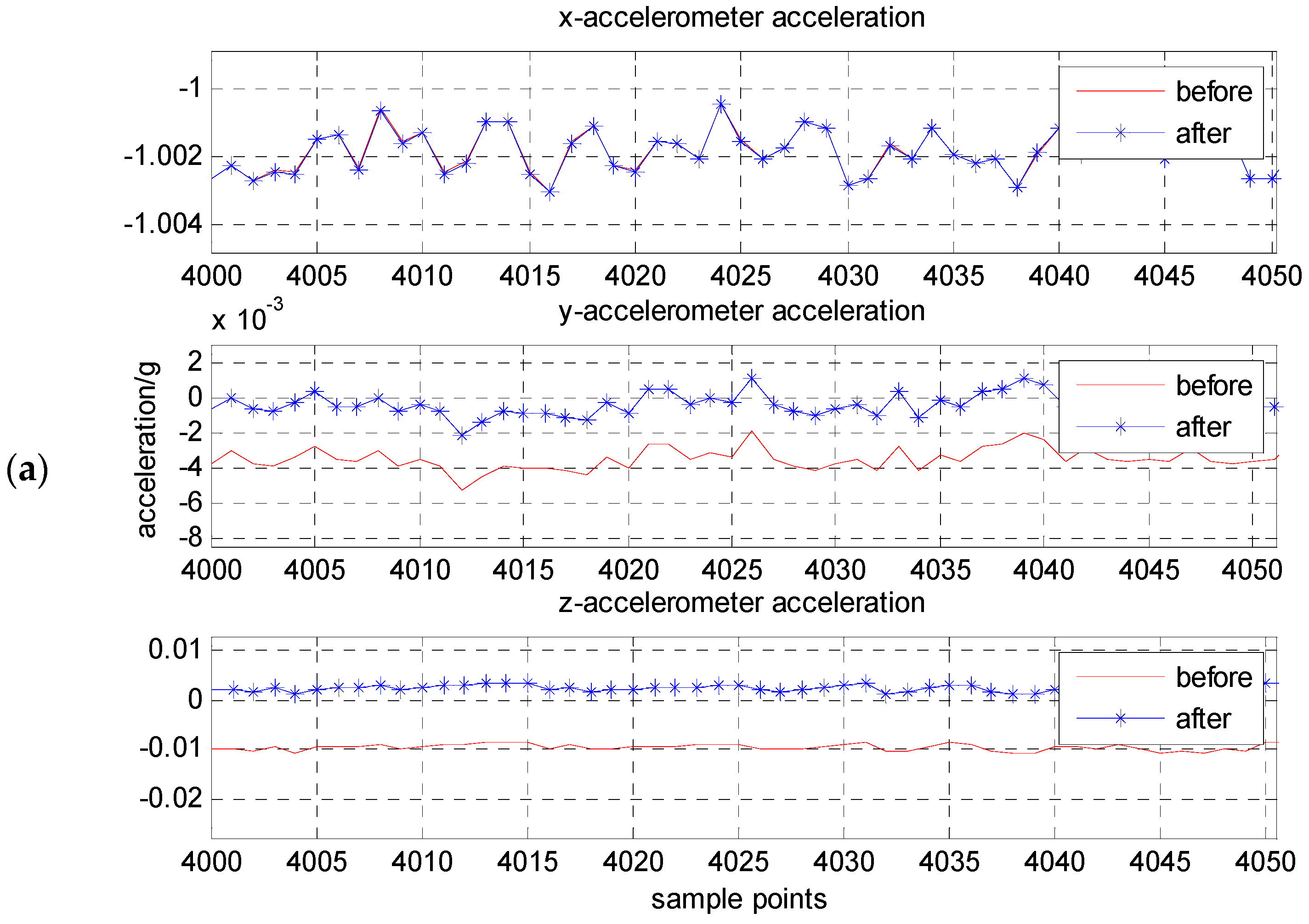
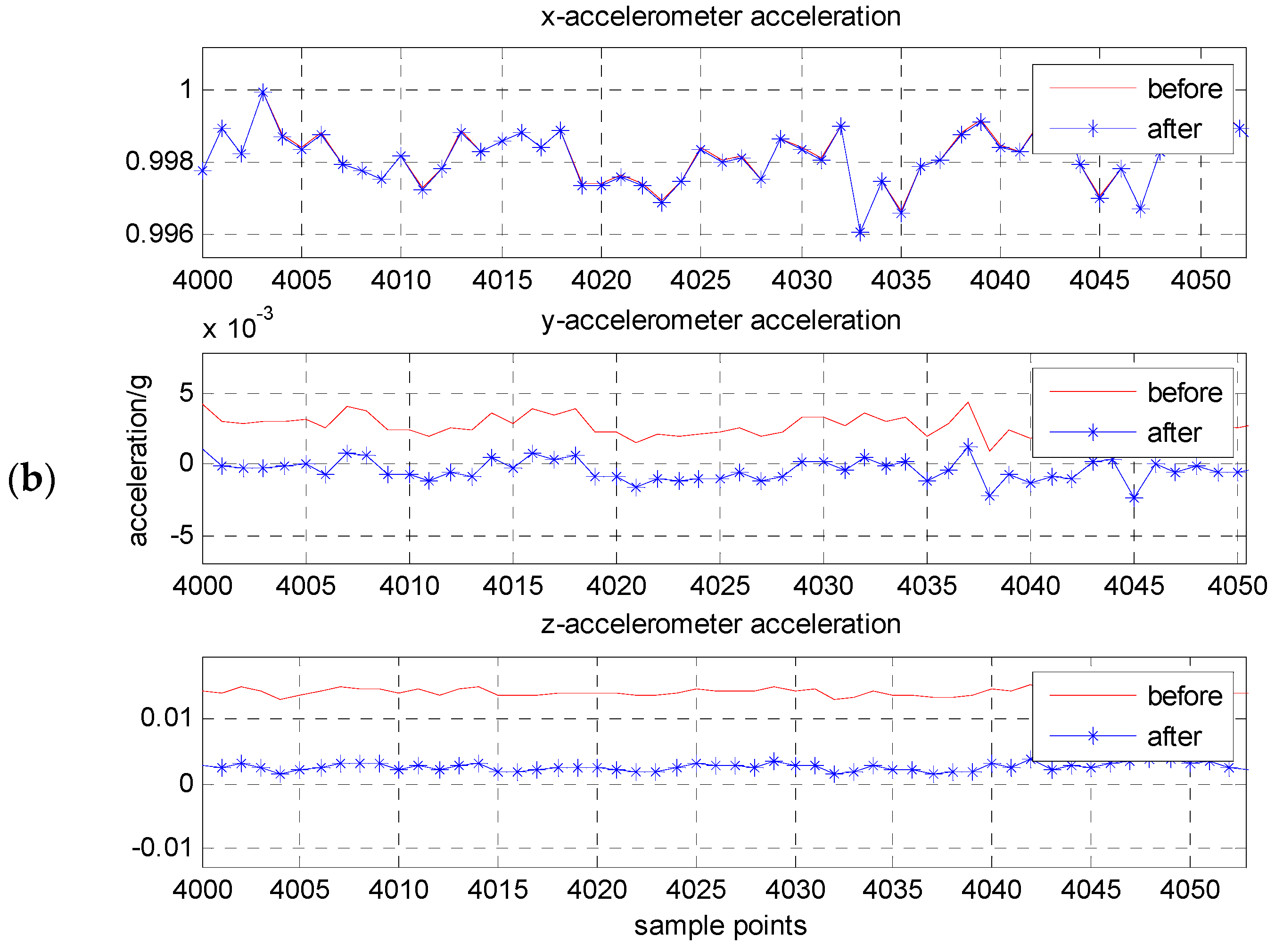
4.2. Dynamic Calibration Result and Discussion
5. Conclusions
Acknowledgments
Author Contributions
Conflicts of Interest
References
- Savage, P.G. Strapdown inertial navigation integration algorithm design part 1: Attitude algorithms. J. Guid. Control Dyn. 1998, 21, 19–28. [Google Scholar] [CrossRef]
- Savage, P.G. Strapdown inertial navigation integration algorithm design part 2: Velocity and position algorithm. J. Guid. Control Dyn. 1998, 21, 208–221. [Google Scholar] [CrossRef]
- Davis, B.S. Using low-cost MEMS accelerometers and gyroscopes as strapdown IMUs on rolling projectiles. In Proceedings of the IEEE Position Location & Navigation Symposium, Palm Springs, CA, USA, 20–23 April 1998; pp. 594–601.
- Aydemir, G.A.; Saranli, A. Characterization and calibration of MEMS inertial sensors for state and parameter estimation applications. Measurement 2012, 45, 1210–1225. [Google Scholar] [CrossRef]
- Peng, H.; Zhi, X.; Wang, R.; Liu, J.Y.; Zhang, C. A new dynamic calibration method for IMU deterministic errors of the INS on the hypersonic cruise vehicles. Aerosp. Sci. Technol. 2014, 32, 121–130. [Google Scholar] [CrossRef]
- Zhu, R.; Zhao, Y.Z. Calibration of three-dimensional integrated sensors for improved system accuracy. Sens. Actuators A 2006, 127, 340–344. [Google Scholar] [CrossRef]
- Yan, M.; Weng, H.N.; Xie, Y. Calibration for system parameters and scaling for installation errors of IMU. J. Chin. Inert. Technol. 2006, 14, 27–29. [Google Scholar]
- Syed, Z.F.; Aggarwal, P.; Goodall, C.; Niu, X.; Sheimy, N. A new multi-position calibration method for MEMS inertial navigation systems. Meas. Sci. Technol. 2007, 18, 897–907. [Google Scholar] [CrossRef]
- Fong, W.T.; Ong, S.K.; Nee, A.Y. Method for in-field use calibration of an inertial measurement unit without external equipment. Meas. Sci. Technol. 2008, 19, 32–38. [Google Scholar] [CrossRef]
- Li, J.; Hong, H.H.; Zhang, W.D. Research on calibration techniques for MEMS-micro inertial measurement unit. Chin. J. Sens. Act. 2008, 21, 1169–1173. [Google Scholar]
- Hwangbo, M.; Kim, J.S.; Kanade, T. IMU self-calibration using factorization. IEEE Trans. Robot. 2013, 29, 493–507. [Google Scholar] [CrossRef]
- Li, C.; Zhang, S.F.; Cao, Y. One new onboard calibration scheme for gimbaled IMU. Measurement 2013, 46, 2359–2375. [Google Scholar] [CrossRef]
- Zhang, X.M.; Chen, G.B.; Li, J. Calibration of triaxial MEMS vector field measurement system. IET Sci. Meas. Technol. 2014, 8, 601–609. [Google Scholar]
- Ma, L.; Chen, W.W.; Li, B. Fast field calibration of MIMU based on the powell algorithm. Sensors 2014, 14, 16062–16081. [Google Scholar] [CrossRef] [PubMed]
- Dar, T.; Suryanarayanan, K.; Geisberger, A. No physical stimulus testing and calibration for MEMS accelerometer. J. Microelectromech. Syst. 2014, 23, 811–818. [Google Scholar] [CrossRef]
- Jan, R.; Martin, S.; Jakub, S. Calibration of low-cost triaxial inertial sensors. IEEE Instrum. Meas. Mag. 2015, 18, 32–38. [Google Scholar]
- Lueken, M.; Misgeld, J.E.; Rueschen, D. Multi-sensor calibration of low-cost magnetic, angular rate and gravity systems. Sensors 2015, 15, 25919–25936. [Google Scholar] [CrossRef] [PubMed] [Green Version]
- Ren, C.H.; Liu, Q.Q.; Fu, T.D. A novel self-calibration method for MIMU. IEEE Sens. J. 2015, 15, 5416–5422. [Google Scholar] [CrossRef]
- Zhang, Z.Q. Two-step calibration methods for miniature inertial and magnetic sensor units. IEEE Trans. Ind. Electron. 2015, 62, 3714–3723. [Google Scholar] [CrossRef]
- Schopp, P.; Graf, H.; Burgard, W. Self-calibration of accelerometer arrays. IEEE Trans. Instrum. Meas. 2016, 65, 1913–1925. [Google Scholar] [CrossRef]
- Yadav, N.; Bleakley, C. Fast calibration of a 9-DOF IMU using a 3 DOF position tracker and a semi-random motion sequence. Measurement 2016, 90, 192–198. [Google Scholar] [CrossRef]


| No. | Zero Bias (V) | Scale Factor (V/g) | Installation Angle (Degree) |
|---|---|---|---|
| 1 | 2.405098 | 0.39496 | (0.75997, 90.71425, 89.74038) |
| 2 | 2.380978 | 0.39808 | (89.25516, 0.74486, 90.5630) |
| 3 | 2.435503 | 0.40024 | (90.52202, 89.17706, 0.97456) |
| Sensor | Theoretical Output | Before Compensation | After Compensation | Before Compensation | After Compensation |
|---|---|---|---|---|---|
| x | ±1 g | 1.00043 | 1.00041 | −0.99956 | −0.99958 |
| y | 0 g | 0.01299 | 0.00098 | −0.01100 | 0.00098 |
| z | 0 g | −0.00911 | 0.00023 | 0.00953 | 0.00020 |
| Installation Position Vector | Installation Position Vector (m) | ||
|---|---|---|---|
| r1 | −0.00834 | −0.00042 | −0.00132 |
| r2 | −0.00256 | −0.00893 | −0.00026 |
| r3 | −0.00060 | −0.00050 | −0.00824 |
| Sensor | Theoretical Output | Before Compensation | After Compensation | Before Compensation | After Compensation |
|---|---|---|---|---|---|
| x | ±1 g | 0.998078 | 0.998060 | −1.001924 | −1.001939 |
| y | 0 g | 0.000289 | 0.000253 | −0.003359 | 0.000253 |
| z | 0 g | −0.014150 | 0.002402 | 0.0093985 | 0.002402 |
© 2017 by the authors. Licensee MDPI, Basel, Switzerland. This article is an open access article distributed under the terms and conditions of the Creative Commons Attribution (CC BY) license ( http://creativecommons.org/licenses/by/4.0/).
Share and Cite
Zhang, X.; Li, J.; Qin, L.; Shen, C. Comprehensive Calibration of Strap-Down Tri-Axis Accelerometer Unit. Micromachines 2017, 8, 68. https://doi.org/10.3390/mi8030068
Zhang X, Li J, Qin L, Shen C. Comprehensive Calibration of Strap-Down Tri-Axis Accelerometer Unit. Micromachines. 2017; 8(3):68. https://doi.org/10.3390/mi8030068
Chicago/Turabian StyleZhang, Xi, Jie Li, Li Qin, and Chong Shen. 2017. "Comprehensive Calibration of Strap-Down Tri-Axis Accelerometer Unit" Micromachines 8, no. 3: 68. https://doi.org/10.3390/mi8030068
APA StyleZhang, X., Li, J., Qin, L., & Shen, C. (2017). Comprehensive Calibration of Strap-Down Tri-Axis Accelerometer Unit. Micromachines, 8(3), 68. https://doi.org/10.3390/mi8030068