ILP-Based and Heuristic Scheduling Techniques for Variable-Cycle Approximate Functional Units in High-Level Synthesis

Abstract

Approximate computing is a promising approach to the design of area–power-performance-efficient circuits for computation error-tolerant applications such as image processing and machine learning. Approximate functional units, such as approximate adders and approximate multipliers, have been actively studied for the past decade, and some of these approximate functional units can dynamically change the degree of computation accuracy. The greater their computational inaccuracy, the faster they are. This study examined the high-level synthesis of approximate circuits that take advantage of such accuracy-controllable functional units. Scheduling methods based on integer linear programming (ILP) and list scheduling were proposed. Under resource and time constraints, the proposed method tries to minimize the computation error of the output value by selectively multi-cycling operations. Operations that have a large impact on the output accuracy are multi-cycled to perform exact computing, whereas operations with a small impact on the accuracy are assigned a single cycle for approximate computing. In the experiments, we explored the trade-off between performance, hardware cost, and accuracy to demonstrate the effectiveness of this work.

1. Introduction

Computational approximation is a promising paradigm that exploits hardware capabilities or mitigates computational demands. Approximate computing is an attractive technique to trade-off high-performance and low-power circuits for applications such as image processing and machine learning, where the applications have an inherent tolerance to errors. This tolerance enables the relaxation of the computation requirement regarding performance or energy because exact computation is not always needed [1,2]. Design techniques for approximate arithmetic circuits have been developed at different design levels, from the transistor to the architecture level [2,3,4,5,6,7,8,9,10,11,12,13,14,15,16]. A variety of techniques for approximate computing have been proposed at the circuit level in the literature, including arithmetic circuits such as approximate adders [6,7,8] and multipliers [9,10,11,12,13]. Approximate computing circuits are generally designed by combining normal (i.e., accurate) functional units with such approximate functional units, based on the requirements for the circuits.

Computational quality (i.e., accuracy) allowed in an application varies in terms of degree of error tolerance, and the degree of approximation for functional units at the circuit level is also different. Approximate functional units have become desirable recently because they enable configuration of the control of accuracy at runtime [8,12,13]. In order to design a circuit that satisfies the requirements in terms of resources and time, in addition to accuracy, it is indispensable to assess how the errors incurred by the approximation circuits propagate via exact and approximate computations, and thus finally affect the output. It is important to discuss this topic, especially for high-level synthesis (HLS) of approximate circuits. Although a large number of studies on HLS of approximate computing circuits have been published [14,15,16], none efficiently utilize such accuracy-controllable functional units.

In this paper, we present a scheduling method that is aware of exact and approximate computations. We mathematically derive a scheduling problem for approximate computing circuits with variable-cycle multipliers based on integer linear programming (ILP), where each arithmetic operation is determined in either exact or approximate mode, and with the degree of approximation (i.e., the number of cycles) during scheduling satisfying resource and time constraints such that the error at the output is minimized. In addition, we extend the problem to take into account operation chaining, which enables the flexible use of approximate computations and further mitigates the output errors. Furthermore, we propose a list-scheduling algorithm for the proposed scheduling problem to obtain an approximate solution in polynomial time.

The main contributions of this paper are twofold:

• Scheduling for approximate computing circuits with accuracy-controllable approximate multipliers is mathematically derived using an ILP formulation. Our proposed scheduling takes account of exact and approximate computations, and determines that each arithmetic operation is scheduled as either exact or approximate under resource and time constraints such that the error at the output is minimized.
• A list-scheduling algorithm is proposed to solve the proposed scheduling problem in polynomial time, which can solve faster than the ILP method.

The remainder of this paper is organized as follows. Section 2 introduces related work. In Section 3, we derive our proposed variable-cycle scheduling problem based on ILP. In addition, we take into account chaining in the scheduling problem. Section 4 proposes a list-scheduling algorithm to efficiently find a solution in polynomial time. Section 5 evaluates our proposed methods. Finally, Section 6 concludes this paper.

2. Related Work

Approximate computing has been established as a promising technique, and several surveys have been reported [1,2,3]. The research on approximate computing has briefly encompassed approximate arithmetic circuits [3,4,5,6,7,8,9,10,11,12,13], logic synthesis [14,15,16,17,18], and modeling [19,20,21,22,23].

According to the review in [3], approximate arithmetic circuits such as approximate adders and multipliers have been introduced. The authors in [6] focused on low-power design, and they developed approximate adders for DSPs to simplify the complexity of a conventional mirror adder cell at the transistor level by adopting approximate computing. As another approach to energy-efficient DSP applications, a reverse carry propagate adder (RCPA) was proposed in [7]. In addition to an approximate adder, the work in [9] developed an approximate multiplier, where the approximate circuits are a bio-inspired imprecise adder and multiplier. In [11], the authors also developed an approximate adder and a multiplier. The proposed multiplier uses the proposed approximate adder for the accumulation of the error signals in the error vectors to reduce the error at the output. Although the mentioned works aimed to purely pursue energy efficiency, high performance, or area reduction at the sacrifice of accuracy, the required accuracy of an error-tolerant application using approximate computing circuits varies significantly at runtime. In previous research [8,12,13], accuracy-controllable approximate arithmetic circuits were developed. The authors in [8] raised the issue that the static approximation, which fixes accuracy, may fail to satisfy the requirements in terms of energy, performance, or area. They sequentially extended their work to propose an accuracy-controllable approximate multiplier [12]. Sano et al. followed these studies to develop a 32-bit accuracy-controllable approximate multiplier for FPGAs [13]. The work aimed to trade-off an approximate computing circuit in terms of energy, performance, and area with respect to the accuracy requirement.

The approximate computing circuits are basically designed with the combination of accurate functional units with approximate functional units [3,4,5,6,7,8,9,10,11,12,13], based on the requirements for the circuits. A number of works have proposed logic synthesis techniques for approximate computing. Nepal et al. proposed automated behavioral synthesis of approximate computing circuits, called ABACUS, which synthesizes an approximate computing circuit by directly operating at the behavioral descriptions of circuits to automatically generate approximate variants [14,15]. Based on their work, Schafer proposed a method that does not use approximate computing circuits but uses exact circuits having lower bandwidths [13]. The author focused on enabling resource-sharing-based design space exploration (DSE) for FPGAs, and did not aim to determine a trade-off between area and error. At the higher level of abstraction, an approximate high-level synthesis (AHLS) was proposed to synthesize a register-transfer-level (RTL) implementation from an accurate high-level C description, which aimed to optimize energy efficiency with voltage scaling [17]. Unlike the works in [16,17], Leipnitz and Nazar proposed an FPGA-oriented approximation methodology that combines with various optimizations, such as precision scaling of operators [14], bitwidth reduction [16], or variable-to-constant (V2C) substitution [17], or uses a set of libraries in [18,24]. The issue has also been addressed from the perspectives of resources, throughput, and real-time operation [25,26,27,28]. In [29], Shirane et al. proposed a case study of high-level synthesis of accuracy-controllable approximate multipliers [12].

Modeling techniques for statistical and analytical perspectives are regarded as significant approaches to approximate computing designs in order to estimate the error produced by approximate circuits [19,20,21,22,23]. Venkatesan et al. proposed a modeling and analysis framework for approximate computing circuits [19]. The drawback of this technique is that it focuses on post-design analysis, and it cannot be easily applied to optimization. In [20], the authors used the error rate, which represents the probability that a result is approximated and different from the exact value, but only addressed the frequency of the error and ignored the magnitude. Some research proposed error propagation rules to overcome this drawback [21,22]. In addition to [21], the authors in [23] proposed a set of analytical models to estimate circuit metrics and a DSE method to derive Pareto-optimal solutions for approximate designs.

Unfortunately, most of the previously mentioned works have paid little attention to allocation, scheduling, and binding algorithms, which are the crucial techniques in HLS. Regarding this perspective, our work is similar to [22,30]. However, none of the previous studies developed scheduling methods that are aware of accuracy-controllable approximate arithmetic circuits. In this work, we focus on scheduling for approximate computing circuits of variable-cycle approximate multipliers. The reason for targeting multipliers is that they are the most common operation in a variety of applications. Although most research involves approximate adders, we deliberately neglect them because the area and delay of a multiplier accounts for a larger portion than those of an adder. Instead, we assume that clock cycles of our approximate multipliers are variable, for which the delay can be controlled by configuring the accuracy. For example, it is assumed that the exact multiplication takes two cycles and the approximate multiplication takes one cycle. The accuracy-controllable multiplier [12,13] can operate with a long delay if an exact multiplication is needed with a single multiplier, or with a short delay if an approximation is good enough. The novelty of our work is the variable cycle of approximate multipliers.

3. ILP-Based Scheduling for Variable-Cycle Approximate Functional Units in High-Level Synthesis

3.1. A Scheduling Example

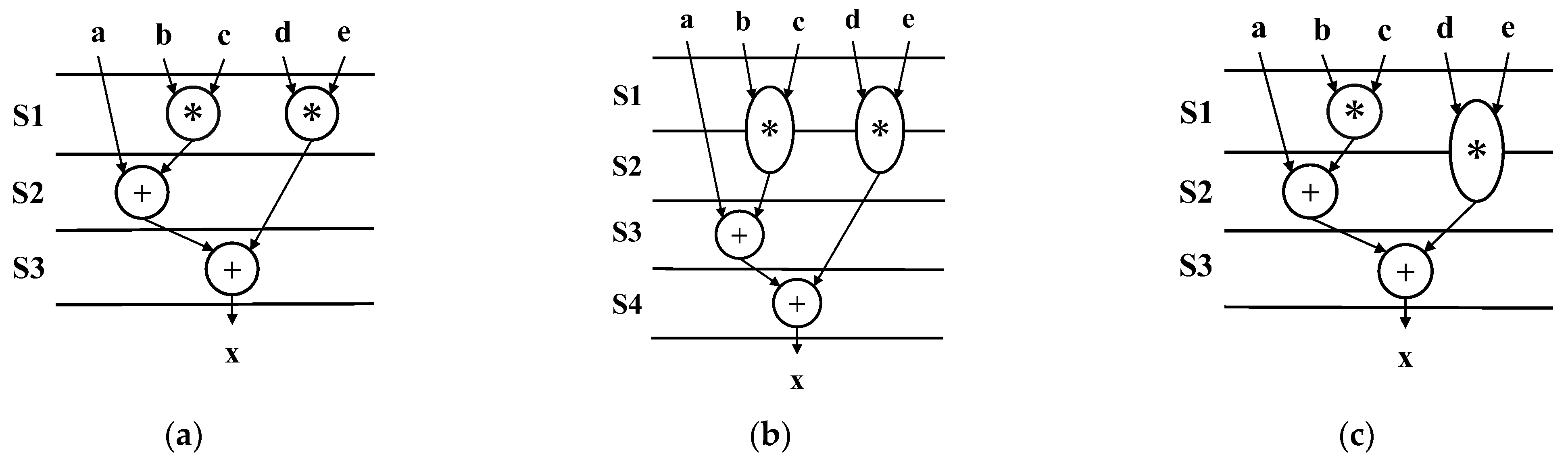
In Figure 1, the three data flow graphs (DFGs) show an example of scheduling. In general, a DFG consists of the nodes and the edges that represent operations and precedence constraints (i.e., data dependencies between the operations), respectively. Each DFG consists of two adders and three multipliers. The notation labeled S means a clock cycle; for instance, S1 is the first clock and S2 is the second clock. In this work, we assume a dual-mode multiplier based on an accuracy-controllable multiplier, which is presented in [12,13]. One mode is used as a normal multiplier that takes two cycles for exact calculation, and the other is an approximate multiplier that takes one cycle. Figure 1a shows that the two multiplications are approximately calculated for each in one cycle, and the whole operation is performed in three cycles. Note that each multiplication in this case takes one cycle, so that the performance is maximized without accounting for accuracy. Therefore, the case in Figure 1a may have a larger error than the case in Figure 1b, where each multiplier performs in two cycles. However, Figure 1b shows four cycles are necessary for all the operations and results in the degradation of performance compared with the case in Figure 1a. Our proposal in Figure 1c is allowed to flexibly employ each multiplier, which is selected as being either exact or approximate. This case demonstrates that one multiplier is approximated, and the others are calculated precisely. The output error should be smaller than the case in Figure 1a. In addition, the total cycle is shown, as well as that in Figure 1b, without the performance degradation. Given the DFG and constraints on the resources and the maximum number of time steps, our proposed scheduling determines each mode of the multipliers and determines an optimal schedule.

3.2. ILP Formulation

Scheduling for variable-cycle approximate functional units is mathematically derived as an ILP formulation in this paper. Given a DFG that consists of functional units and data flow dependencies, scheduling determines the number of cycles for each operation under time and resource constraints such that the error at the output is minimized. We assume that the multipliers are accuracy-controllable, and can be selected as being in either exact or approximate mode. The exact mode yields accurate output, but the approximate mode outputs an inaccurate result. The approximate mode of a multiplier can vary its own cycles, and scheduling also determines the number of cycles for each multiplication.

Let ${\mathit{mul}}_{i,k}$ denote a binary decision variable to schedule the $i$-th multiplication in the $k-\mathrm{th}$ cycle. If ${\mathit{mul}}_{i,k}$ becomes 1, multiplication $i$ is being performed in the $k-\mathrm{th}$ cycle. Similarly, let $o{p}_{j,k}$ denote a binary decision variable to schedule the $j-\mathrm{th}$ operation other than multiplication in the $k-\mathrm{th}$ cycle. Each multiplication is determined in either the approximate or exact mode and takes one cycle or several cycles. The number of cycles for the multiplication is varied dependent on the degree of approximation. The delay produced by the other operations is relatively shorter than that of the multiplication. For simplicity, we have classified the operations as multiplication and the other operations, but we can prepare an operation other than multiplication with a variable cycle, which does not essentially make any difference.

Here, we define the number of cycles for each multiplication and the other operations. For comprehension, we assume in Equations (1) and (2) that $mu{l}_{i,k}$ takes either one or two cycles and $o{p}_{j,k}$ takes one cycle. However, the number of cycles for $mu{l}_{i,k}$ and $o{p}_{j,k}$ can be easily extended as a decision variable and an arbitrary number of cycles, respectively.

$$\forall i,({\sum }_k{\mathit{mul}}_{i,k}=1) \vee ({\sum }_k{\mathit{mul}}_{i,k}=2)$$

(1)

$$\forall j,{\sum }_{k}o{p}_{j,k}=1$$

(2)

Let $cycle\_mu{l}_i$, $start\_mu{l}_i$, $finish\_mu{l}_i$ denote the number of cycles, the start time, and the finish time of $i$-th multiplication, respectively. Each multiplication is assumed to be performed in one or two cycles, and the start time and finish time are the same if the multiplication is determined to be performed in one cycle.

$$\forall i,{\sum }_k{\mathit{mul}}_{i,k}{=\mathit{cycle}\_\mathit{mul}}_i$$

(3)

$$\forall i, k,\max {\left(k·{\mathit{mul}}_{i,k}\right)}_i{=\mathit{finish}\_\mathit{mul}}_i$$

(4)

$$\forall i,\left({\mathit{finish}\_\mathit{mul}}_i-{1=\mathit{start}\_\mathit{mul}}_i\right) \vee { (\mathit{finish}\_\mathit{mul}}_i{=\mathit{start}\_\mathit{mul}}_i)$$

(5)

$$\forall i,{\mathit{finish}\_\mathit{mul}}_i-{\mathit{start}\_\mathit{mul}}_i{+1=\mathit{cycle}\_\mathit{mul}}_i$$

(6)

Next, let $time\_o{p}_j$ denote the number of cycles for the $j$-th operation other than multiplication. On the assumption that $al{u}_{j,k}$ takes only one cycle in the description, we can easily extend the number of cycles to an arbitrary number of cycles with similar equations to Equations (3)–(6).

$$\forall j,k,\max {\left(k·o{p}_{j,k}\right)}_j=time\_o{p}_j$$

(7)

The DFG, which is given as an input, includes precedence constraints between the operations. Let ${\mathit{Flow}}_{i1,i2}$ denote a binary value of the dependency between $i1$-th and $i2$-th operations. If ${\mathit{Flow}}_{i1,i2}$ is given as one, there are the constraints between $i1$-th and $i2$-th operations. Equation (8) indicates that the start time of the successor operation $i2$ must be followed after the finish time of the predecessor operation i1. The constraints for operations other than multiplication can be easily taken into account by adding equations similar to Equation (8).

$$\forall i1, i2,{\mathit{Flow}}_{i1,i2} \to { \mathit{finish}\_\mathit{mul}}_{i1}+1 \le { \mathit{start}\_\mathit{mul}}_{i2}$$

(8)

Most of the scheduling requires resource and time constraints. Both of the constraints are assumed to be given in advance. The resource constraints for the multiplication and other operations are fixed as $\mathit{MULmax}$, and then the number of multipliers is limited. The number of the multipliers assigned to active multiplications cannot exceed the number of the total number of multipliers in any cycle $k$ as follows. Assume unlimited availability for the purpose of avoiding overhead in sharing, except for multipliers such as adders and ALUs.

$$\forall k,{\sum }_i{\mathit{mul}}_{i,k} \le \mathit{MULmax}$$

(9)

Furthermore, the time constraints are given as $\mathit{TIMEconst}$, which limit the finish time of multipliers and other operations. All the operations must finish performing before the time constraint. Let $finish\_o{p}_j$ denote the finish time of the $j-\mathrm{th}$ operation other than multiplication. In this paper, $finish\_o{p}_j$ and $time\_o{p}_j$ are synonymous because it is assumed that operations other than multiplication can be performed in one cycle. The time constraints are given as follows:

$$\forall i,1 \le { \mathit{finish}\_\mathit{mul}}_i \le \mathit{TIMEconst}$$

(10)

$$\forall j 1 \le finish\_o{p}_j\le \mathit{TIMEconst}$$

(11)

Accuracy is evaluated by the magnitude of the error. In other words, the smaller the error, the higher the accuracy of the circuit. We describe how errors are produced if the operations are approximated, using a multiplication operation. Consider multiplication operation $p=a\times b$. Let the errors propagated before $a$ and $b$ be denoted as ${\epsilon }_a$ and ${\epsilon }_b$, and the errors of the multiplication and its product be denoted as ${\epsilon }_{*}$ and ${\epsilon }_p$, respectively. Here, we derive the approximate multiplication in Equation (12). It should be noted that ${\epsilon }_a{\epsilon }_b$ can be ignored due to negligible loss of accuracy, as in [21,22].

$$p+{\epsilon }_p=a\cdot b+a{\epsilon }_b+b{\epsilon }_a+{\epsilon }_{+}\sout{+{\epsilon }_a{\epsilon }_b}$$

(12)

Based on the assumption, let ${\mathsf{\epsilon }\_\mathit{mul}}_i$ denote the errors produced in the $i$-th multiplication. Let ${\mathsf{\epsilon }}_i$ denote an error generated if the $i$-th multiplication is approximated and becomes non-zero if the multiplication is approximated. In other words, ${\mathsf{\epsilon }}_i$ is zero if multiplication $i$ is exactly performed without approximation. Note that Equation (13) assumes that the exact multiplication takes two cycles. However, it can easily be extended to take an arbitrary number of cycles if the error that increases in a linear manner with the increase in the degree of approximation is allowed. The same formulation is also used for operations other than multiplication.

$$\forall i,{\mathsf{\epsilon }\_\mathit{mul}}_i=a·{\mathsf{\epsilon }}_b+b·{\mathsf{\epsilon }}_a+(2-{\mathit{cycle}\_\mathit{mul}}_i{)\mathsf{\epsilon }}_i$$

(13)

Let ${\epsilon }_o$ denote the error at the output, which means the error produced by a final output of the operation, either ${\mathsf{\epsilon }\_\mathit{mul}}_i$ or the error of other operations. The error at the output derives from each error propagated from each of the operations. In this work, the objective of our scheduling is to minimize the error at the output.

$$\mathrm{Minimize} {\mathsf{\epsilon }\_\mathit{mul}}_i=a·{\mathsf{\epsilon }}_b+b·{\mathsf{\epsilon }}_a+(2-{\mathit{cycle}\_\mathit{mul}}_i{)\mathsf{\epsilon }}_i$$

(14)

We formulate this problem as ILP and can solve it using an ILP solver. In this work, the multiplications are performed in one or two cycles; however, the presented formulation can be easily changed to be performed in any number of cycles.

3.3. Chaining

Scheduling algorithms for high-level synthesis that cannot handle optimization techniques are of no practical value. Among the several optimization techniques that exist, we consider chaining in this work. For the proposed method, the aim of chaining is to speed up the circuit and improve the computational accuracy by increasing the number of accurate multiplications.

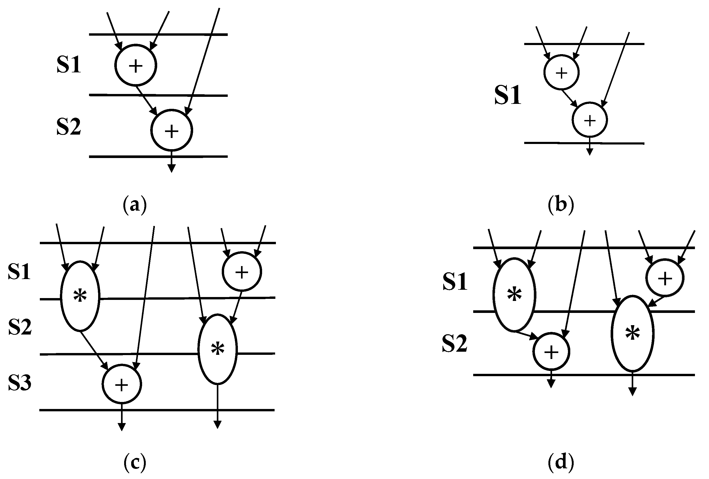
The chaining assumed in this work is shown in Figure 2. We assume two types of chaining. The first is general addition chaining, in which the number of stages is changed based on the given delay constraints. Without considering addition chaining, it takes two cycles to perform two additions, as shown in Figure 2a. If two adders are used, as in Figure 2b, it can be performed in one cycle. Thus, the configuration of the functional unit is important when performing chaining. Next, we consider not only the chaining of additions, but also the chaining of exact multiplications and additions. Here, we assume that exact multiplication is performed in two cycles. If chaining is not considered, it takes three cycles, as shown in Figure 2c. If we perform exact multiplication and addition with chaining, it can be performed in two cycles, as shown in Figure 2d. Since the scheduling problem in this work is to minimize the error under the constraints of resources and time, we predict that exact multiplication and addition chaining will have a significant impact on the error reduction.

The important point in chaining is which operations are chained. In particular, under resource constraints, the overall number of execution cycles differs greatly depending on which operations are chained. In the ILP method, the following changes are made to some equations to take chaining into account.

First, in the ILP method without considering chaining, Equations (1) and (2) were classified into multiplication and non-multiplication operations. However, these are classified into multiplication, addition, and other operations by adding Equation (15). Let $ad{d}_{m,k}$ be a 0–1 decision variable that is $m$ when addition $m$ is performed in cycle $k$. Moreover, let ${\mathit{time}\_\mathit{add}}_m$ be the execution time of addition $m$. Thus, addition is defined as in Equations (15) and (16), and time constraints are defined as in Equation (17), as in ILP without considering chaining. To avoid sharing overhead, an unlimited number of adders are assumed to be available.

$$\forall m, k {\sum }_k{\mathit{add}}_{m,k} = 1$$

(15)

$$\forall m, k, \max {\left(k·{\mathit{add}}_{m,k}\right)}_{\mathrm{l}}{ = \mathit{time}\_\mathit{add}}_m$$

(16)

$$\forall m, 1 \le { \mathit{time}\_\mathit{add}}_m \le \mathit{TIMEconst}$$

(17)

Let $add\_ste{p}_m$ be the number of steps when chaining additions together, and let STEP be the maximum number of steps that an addition can chain. To avoid chaining beyond the delay condition, STEP is defined from the delay condition.

$$\forall m, 1 \le { \mathit{add}\_\mathit{step}}_m \le \mathit{STEP}$$

(18)

We also make changes to the dependencies. In the case of the dependency between additions, it is defined as in Equation (19). In the case of no chaining, the two additions are executed in different cycles. In the case of chaining, the two additions are performed in the same cycle.

$$\begin{gathered} \forall m1,m2, {\mathit{Flow}}_{m1,m2}\to {(\mathit{time}\_\mathit{add}}_{m1} + 1 \le { \mathit{time}\_\mathit{add}}_{m2} \&\&{ \mathit{add}\_\mathit{step}}_{m2}= \\ 1) ||{ (\mathit{time}\_\mathit{add}}_{m1}{=\mathit{time}\_\mathit{add}}_{m2} \&\&{ \mathit{add}\_\mathit{step}}_{m1} + 1 \le { \mathit{add}\_\mathit{step}}_{m2}) \end{gathered}$$

(19)

The dependency between addition and multiplication is defined as in Equations (20) and (21). Equation (20) shows the dependency from multiplication to addition and Equation (21) shows the dependency from addition to multiplication. Define ${\mathit{mul}\_\mathit{chain}}_{i1}$ as 1 for chaining from exact multiplication to addition, and 2 for chaining from addition to exact addition. As in the case of chaining between additions, it is performed in different cycles when not chaining, and in the same cycle when chaining. Approximate multiplication is not performed using chaining in this work.

$$\begin{gathered} \forall m1,i1, {\mathit{Flow}}_{i1,m1}\to {(\mathit{finish}\_\mathit{mul}}_{i1} + 1 \le { \mathit{time}\_\mathit{add}}_{m1}) || ({\mathit{finish}\_\mathit{mul}}_{i1} + 2 - \\ { \mathit{cycle}\_\mathit{mul}}_i{=\mathit{time}\_\mathit{add}}_{m1} \&\& {\mathit{mul}\_\mathit{chain}}_{i1} = 1 \end{gathered}$$

(20)

$$\begin{gathered} \forall m1,i1, {\mathrm{Flow}}_{m1,i1}\to {(\mathit{time}\_\mathit{add}}_{m1} + 1 \le { \mathrm{start}\_\mathit{mul}}_{i1}) || ({\mathit{time}\_\mathit{add}}_{m1} + 2 - \\ { \mathit{cycle}\_\mathit{mul}}_i{ = \mathrm{start}\_\mathit{mul}}_{i1} \&\& {\mathit{mul}\_\mathit{chain}}_{i1}=2 \end{gathered}$$

(21)

4. Heuristic Scheduling Algorithms Based on List Scheduling

4.1. List-Scheduing Algorithm

Table 1. Symbols for list-scheduling algorithm.

G(V,E)	Data Flow Graph (DFG)
V	Set of operations
E	Set of data dependencies between operations
M	Set of multiplications ($\mathrm{M}\subseteq \mathrm{V}$)
A	Set of operations other than multiplication (A$\subseteq \mathrm{V}$)
$\mathrm{Apx}$	Set of approximate multiplications $(\mathrm{Apx}\subseteq \mathrm{M}$)
${\mathrm{M}}^{\prime }$	Set of multiplications that have never been performed as exact multiplications $({\mathrm{M}}^{\prime }\subseteq \mathrm{M})$
$\sigma$	Set of operations that can be executed
$\tau$	Set of operations that are being executed (set of operations currently running in multi-cycle)
$\pi$	Set of operations that have completed execution
$T_{\mathit{apx}}$	Number of cycles required for approximate multiplication
$T_{\mathit{res}}$	Number of cycles required for exact multiplication
$T_{\mathit{op}}$	Number of cycles required for operations other than multiplication
$i$	i-th of all operations
$t$	Current clock cycle
${\mathit{ts}}_i$	Execution start time of the i-th operation
${\mathit{tf}}_i$	Execution finish time of the i-th operation
${\mathit{tr}}_i$	Remaining time until the end of the execution of the i-th operation
${\mathit{Const}}_{\mathit{mul}}$	The number of available multipliers (resource constraints)
${\mathit{Const}}_{\mathit{time}}$	The number of execution cycles for the entire circuit (time constraint)
$N_{\mathit{mul}}$	Remaining number of multipliers available for the current clock cycle
${t\_\mathit{alap}}_i$	Execution time of the i-th operation in ALAP (result of ALAP)
${\mathit{res}}_i$	Exact value of the i-th operation
${\mathit{err}}_i$	Error of the i-th operation
$e_i$	The magnitude of error given to the final output when approximating the i-th operation
$p_i$	Priority based on ALAP results
$T_{add}$	Number of cycles required for addition
$j$	i-th of addition
$\mathit{Condition}\_\mathit{chaining}\_\mathit{mul}$	Value indicating whether exact multiplication and addition can be performed chaining
$\mathit{Condition}\_\mathit{chaining}\_\mathit{add}$	Value indicating whether additions can be performed chaining
$\mathrm{D}$	Set of additions

shows the symbols used in the list scheduling. We propose a heuristic algorithm for the variable-cycle scheduling problem and show pseudo-code based on the conventional resource-constrained list scheduling in Algorithm 1. For a given DFG G(V,E), let $\mathrm{V}$, $\mathrm{M}$, $\mathrm{A}$, and $\mathrm{Apx}$ be the set of all operations, i.e., multiplication, operations other than multiplication, and approximate multiplication, respectively. In this case, $\mathrm{V}=\mathrm{M}\cup \mathrm{A}$ and $\mathrm{Apx} \subseteq \mathrm{M}$. Let $\sigma$ denote the operations that can be executed, $\tau$ denote the operations that are being executed, and $\pi$ denote the operations that have completed execution. Initially, $\pi ,\tau =\{\varnothing \}$. The length of the number of execution cycles for approximate multiplication, exact multiplication, and other operations is $T_{\mathit{apx}}{, T}_{\mathit{res}},$ and $T_{\mathit{op}}$, respectively. These are given as preconditions. Let ${t\_\mathit{alap}}_i$ be the execution cycle of each operation calculated by As Late As Possible (ALAP). Let $p_i$ be the priority of the list scheduling to be created based on it. Let the start time of each operation $i$ be ${\mathit{ts}}_i$ and the end time be ${\mathit{tf}}_i$. If the operation is executed in a single cycle, these will be the same values. Let ${\mathit{tr}}_i$ be the remaining time until the execution of operation $i$ is completed, and $t$ be the current cycle. In the constraints, i.e., resource constraints and time constraints, ${\mathit{Const}}_{\mathit{mul}}$ limits the number of multipliers and ${\mathit{Const}}_{\mathit{time}}$ limits the overall number of execution cycles. The number of currently available multipliers is defined as $N_{\mathit{mul}}$. This is updated every cycle. Let $e_i$ be an index of the magnitude of the error given to the output value when approximating the multiplication. This value is obtained from the calculation of error propagation. To minimize the output error, scheduling is performed by switching to the exact mode in order of the multiplication with the largest error. The set of multiplications that have never been made exact is denoted as ${\mathrm{M}}^{\prime }$, and we loop until all the multiplications have been made exact once. In the initial state, ${\mathrm{M}}^{\prime }=\mathrm{M}$.

Algorithm 1 List-Scheduling Algorithm
1	ListScheduling(G(V,E)) begin
2	for $i\in \mathrm{V}$ do
3	${t\_\mathit{alap}}_i$ ← ALAP_schedule
4	end for
5	for $i\in \mathrm{V}$ do
6	$e_i\leftarrow { \mathrm{Obtain} \mathit{res}}_i{, \mathit{err}}_i \mathrm{from} \mathrm{G}\left(\mathrm{V},\mathrm{E}\right) \mathrm{and} \mathrm{any} \mathrm{input}$
7	end for
8	for n in 1..|M|+1 do
9	for $i\in \mathrm{V}$ do
10	if $i\in \mathrm{A}{\displaystyle \cup }i\in \mathrm{Apx}$ then
11	$p_i{=t\_\mathit{alap}}_i$
12	else $p_i{=t\_\mathit{alap}}_i-{(T}_{\mathit{res}}-T_{\mathit{apx}})$ end if
13	end for
14	$t$ = 0,$\pi = \{\varnothing \}, \tau = \{\varnothing \}$
15	while $\pi \ne \mathrm{V}$ do
16	$N_{\mathit{mul}}{ = \mathit{Const}}_{\mathit{mul}}, t++$
17	for $i\in \mathrm{V}$ do
18	for $i\in \tau$ do
19	if $i\in \mathrm{M}$ then
20	${\mathit{tr}}_i{ = \mathit{tr}}_i-{1, N}_{\mathit{mul}}{ = N}_{\mathit{mul}}-1$
21	if $t{r}_i = 0$ then
22	$\pi =\pi \cup i$, $\tau =\tau \cap { \neg i, \mathit{tf}}_i=t$
23	$\sigma \leftarrow \mathrm{successor} \mathrm{nodes} \mathrm{of} \mathrm{operation} i \mathrm{in} \mathrm{V}$
24	end if
25	end if
26	if $i\in \mathrm{A}$ then
27	${\mathit{tr}}_i{=\mathit{tr}}_i-1$
28	if ${\mathit{tr}}_i=0$ then
29	$\pi =\pi \cup i$, $\tau =\tau \cap \neg i$, ${\mathit{tf}}_i=t$
30	$\sigma \leftarrow \mathrm{successor} \mathrm{nodes} \mathrm{of} \mathrm{operation} i \mathrm{in} \mathrm{V}$
31	end if
32	end if
33	end for
34	if $N_{\mathit{mul}} \ge 1\cap \left\{i\right|i\in \left(\sigma \cap M\right)\cap \min (p_i\left)\right\}$ then
35	$t{s}_i=t$, $N_{\mathit{mul}}{=N}_{\mathit{mul}}-1, \sigma =\sigma \cap \neg i$
36	if $i\in \mathrm{Apx} \cap { T}_{\mathit{apx}}=1$ then
37	$\pi =\pi \cup i$, ${\mathit{tf}}_i=t$
38	$\sigma \leftarrow \mathrm{successor} \mathrm{nodes} \mathrm{of} \mathrm{operation} i \mathrm{in} \mathrm{V}$
39	elif $i\in \mathrm{Apx} \cap { T}_{\mathit{apx}}\text{>}1$ then
40	$\tau =\tau \cup i$, ${\mathit{tr}}_i{=T}_{\mathit{apx}}-1$
41	else $\tau =\tau \cup i$, ${\mathit{tr}}_i{=T}_{\mathit{res}}-1$ end if
42	end if
43	if $\left\{i\right|i\in \left(\sigma \cap \mathrm{A}\right)\cap {\min (p}_i\left)\right\}$ then
44	${\mathit{ts}}_i=t, \sigma =\sigma \cap \neg i$
45	if $i\in \mathrm{A} \cap { T}_{\mathit{op}}=1$ then
46	$\pi =\pi \cup i$, ${\mathit{tf}}_i=t$
47	$\sigma \leftarrow \mathrm{successor} \mathrm{nodes} \mathrm{of} \mathrm{operation} i \mathrm{in} \mathrm{V}$
48	else $\tau =\tau \cup i$, ${\mathit{tr}}_i{=T}_{\mathit{op}}-1,$ end if
49	end if
50	end for
51	end while
52	if $\forall {i, \mathit{tf}}_i \le { \mathit{Const}}_{\mathit{time}}$ then
53	${\mathit{best}\_\mathit{ts}}_i{=\mathit{ts}}_i$,${ \mathit{best}\_\mathit{tf}}_i{=\mathit{tf}}_i, \mathit{best}\_ \mathrm{Apx}=\mathrm{Apx}$
54	$\{{\mathrm{M}}^{\prime }={\mathrm{M}}^{\prime }\cap \neg i\}\cap \left\{i\right|i\in {\mathrm{M}}^{\prime }\cap {\max (e}_i\left)\right\}$
55	else $\{\mathrm{Apx}=\mathrm{Apx}\cup i\}\cap \left\{i\right|i\in {\mathrm{M}}^{\prime }\cap {\max (e}_i\left)\right\}$
56	$\{{\mathrm{M}}^{\prime }={\mathrm{M}}^{\prime }\cap \neg i\}\cap \left\{i\right|i\in {\mathrm{M}}^{\prime }\cap {\max (e}_i\left)\right\}$
57	end if
58	$\{\mathrm{Apx}=\mathrm{Apx}\cap \neg i\}\cap \left\{i\right|i\in {\mathrm{M}}^{\prime }\cap {\max (e}_i\left)\right\}$
59	end for
60	end

In Algorithm 1, ALAP scheduling is first performed in line 3. Here, all the multiplications are scheduled as approximate multiplications. This result is used as a priority when performing resource-constrained list scheduling from line 8. Next, line 6 finds the multiplication whose error becomes large if it is approximated by calculating the error propagation, and finds its influence $e_i$. Between line 8 and line 59, if all the multiplications are approximate multiplications or if they are exact one-by-one multiplications, the total number of multiplications plus one time resource-constrained list scheduling is performed. Scheduling is performed to minimize the error under resource and time constraints. As a new change, in line 12, we reduce the priority used for resource-constrained list scheduling only for exact multiplications. This is to avoid performing ALAP again when some of the multiplications are switched to the exact mode and to make it easier to satisfy the time constraints. Lines 18 to 35 process the multicycle operations that are being executed. Lines 36 to 51 execute the operations with the highest priority among the operations that can be executed. After executing all the operations, satisfaction of the time constraint is checked at line 52. If it satisfied, it is retained as the best solution. If not, the exact multiplication is returned to approximate multiplication. Finally, the approximate solution that satisfies the resource and time constraints and minimizes the error is output. The computational complexity of this algorithm is ${\mathrm{O}(\mathrm{n}}^2\mathrm{logn})$ because the list scheduling is repeated one time plus the number of multiplications.

4.2. Proposed List-Scheduling Example

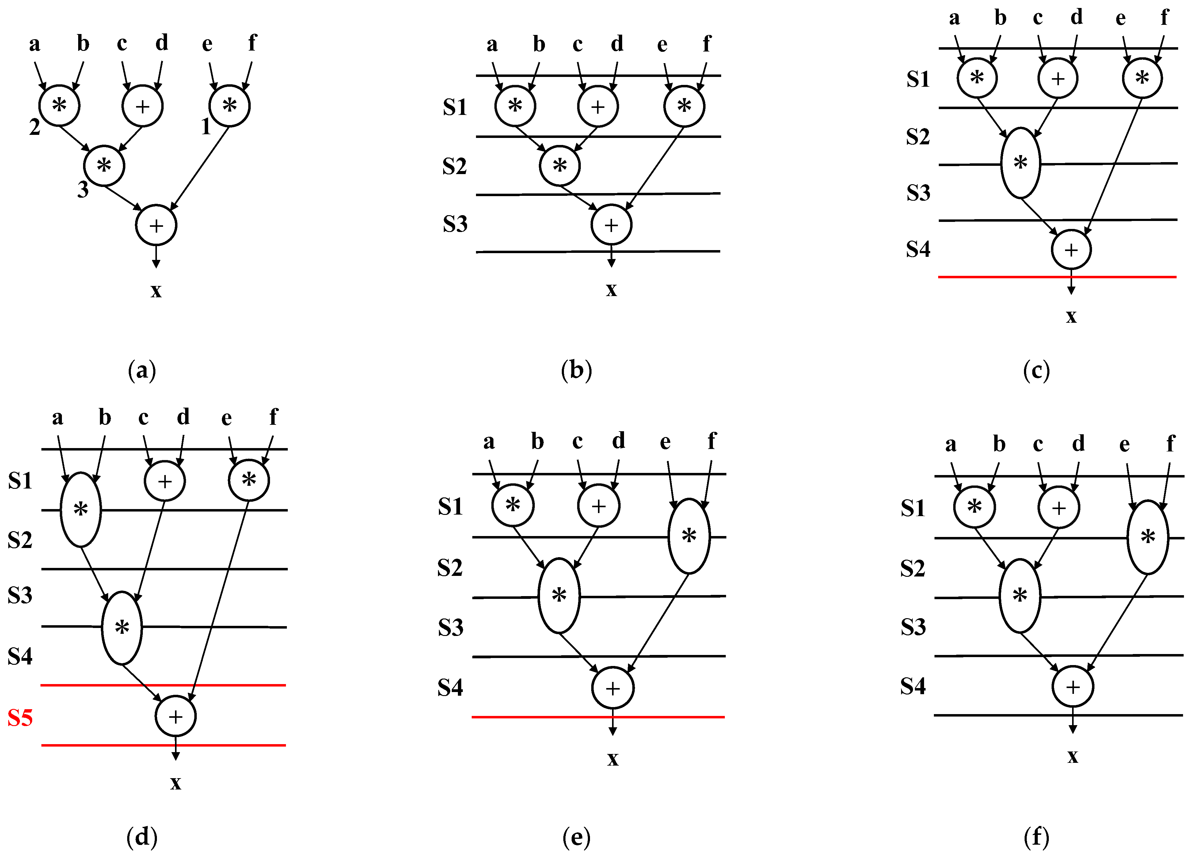
For the operation from lines 8 to 59 of Algorithm 1, an example problem in DFG with three multiplications and two additions is shown in Figure 3. We assume one cycle for approximate multiplications, two cycles for exact multiplications, and one cycle for additions. The resource constraint is list scheduling as two accuracy-controllable approximate multipliers and one adder. The time constraint is four cycles. Figure 3a shows the DFG given, and the number at the bottom left of the multiplication is assumed to be the magnitude of the influence of the error on the output value obtained in line 6 of Algorithm 1. First, as shown in Figure 3b, all the multiplications are approximate multiplications, and resource constraint-based list scheduling is performed. Next, the list scheduling is performed again with the multiplications made exactly with the largest errors. At this time, since all the operations can be performed within the time constraint of four cycles, the multiplication that was made exact in Figure 3c is kept exact for the next scheduling. Next, as shown in Figure 3d, the multiplication with the second-largest error is made exact and list scheduling is performed. However, in Figure 3d the time constraint of four cycles is exceeded, so the upper left multiplication is returned to approximation. Next, the multiplication with the smallest error is made exact and list scheduling is performed. The result of Figure 3e satisfies the time constraint, so we keep the multiplication as exact. Finally, since all the multiplications have been performed correctly, the result of Figure 3e, which will have the smallest error so far, is output as the final solution as shown in Figure 3f. In this example, we show 1–2 cycles for simplicity, but our proposed method can be applied to operations with more than 3 cycles by changing the values of $T_{\mathit{res}}$ and $T_{\mathit{apx}}$.

4.3. Chaining

List scheduling takes chaining into account by adding the following process. Similar to ILP, list scheduling classifies operations into three categories: multiplication, addition, and others. Algorithms 2 and 3 are the additions to of list scheduling, where $\mathrm{D}$ is the set of additions. $T_{add}$ is the length of the execution cycle of the additions. Algorithm 2 is added after line 25 and Algorithm 3 is added after line 42 to perform resource constraint-based list scheduling. It also assumes that an unlimited number of adders are available to avoid sharing overhead as in ILP.

Algorithm 2 Add in List-Scheduling Algorithm ①
1	if$i\in \mathrm{D}$then
2	${\mathit{tr}}_i{ = \mathit{tr}}_i-1,$
3	if ${\mathit{tr}}_i = 0$ then
4	$\pi = \pi \cup i$, $\tau = \tau \cap \neg i$, ${\mathit{tf}}_i = t$
5	$\sigma \leftarrow \mathrm{successor} \mathrm{nodes} \mathrm{of} \mathrm{operation} i \mathrm{in} \mathrm{V}$
6	End if
7	End if

Algorithm 3 Add in List-Scheduling Algorithm ②
1	if$\left\{i\right|i\in \left(\sigma \cap \mathrm{D}\right)\cap {\min (p}_i\left)\right\}$then
2	${\mathit{ts}}_i=t, \sigma = \sigma \cap \neg i$
3	if $i\in \mathrm{D} \cap { T}_{add}=1$ then
4	$\pi = \pi \cup i$, ${\mathit{tf}}_i = t$
5	$\sigma \leftarrow \mathrm{successor} \mathrm{nodes} \mathrm{of} \mathrm{operation} i \mathrm{in} \mathrm{V}$
6	else $\tau =\tau \cup i$, ${\mathit{tr}}_i{ = T}_{add}-1,$ end if
7	End if

Moreover, Algorithm 4 is added after Algorithm 1 to the chaining process. Three chaining processes are performed in sequence: exact multiplication to addition, addition to exact multiplication, and addition to addition.$\mathit{Condition}\_\mathit{chaining}\_\mathit{mul}$ is a value that indicates whether chaining is possible based on the delay condition of exact multiplication. When this value is 1, exact multiplication and addition can be chained, and when it is 0, chaining is not possible. Similarly, let $\mathit{Condition}\_\mathit{chaining}\_\mathit{add}$ be a value that indicates whether or not chaining is possible between additions based on the delay condition of the addition.

Algorithm4 Chaining in List-Scheduling Algorithm
1	if$\mathit{Condition}\_\mathit{chaining}\_\mathit{mul} = 1$then
2	for $i\in \mathrm{V}$ do
3	if ${\displaystyle \cap }\{i\in \mathrm{M},\pi \cap { \mathit{tf}}_i = t \cap i \mathrm{followed} \mathrm{by} j\in \mathrm{D}\}$ then
4	${\mathit{ts}}_j = t, \sigma = \sigma \cap \neg i$
5	if $j\in \mathrm{D} \cap { T}_{add} = 1$ then
6	$\pi = \pi \cup j$, ${\mathit{tf}}_j = t$
7	$\sigma \leftarrow \mathrm{successor} \mathrm{nodes} \mathrm{of} \mathrm{op} j \mathrm{in} \mathrm{V}$
8	else $\tau = \tau \cup j$, ${\mathit{tr}}_j{ = T}_{add}-1,$ end if
9	end if
10	if ${\mathrm{N}}_{mul}\ge 1{\displaystyle \cap }\{i\in \mathrm{D},\pi \cap {\mathit{tf}}_i = t\cap i \mathrm{followed} \mathrm{by} j\in \mathrm{M}\}$ then
11	${\mathit{ts}}_i = t$, ${\mathrm{N}}_{mul}{ = \mathrm{N}}_{mul}-1, \sigma = \sigma \cap \neg i$
12	if $i\in \mathrm{M} \cap { T}_{res} = 1$ then
13	$\pi = \pi \cup i$, ${\mathit{tf}}_i = t$
14	$\sigma \leftarrow \mathrm{successor} \mathrm{nodes} \mathrm{of} \mathrm{op} i \mathrm{in} \mathrm{V}$
15	else $\tau = \tau \cup i$, ${\mathit{tr}}_i{ = T}_{res}-1,$ end if
16	end if
17	end for
18	end if
19	if$\mathit{Condition}\_\mathit{chaining}\_\mathit{add} = 1$then
20	for $i\in \mathrm{V}$ do
21	if $\{i\in \mathrm{D},\pi \cap {\mathit{tf}}_i = t\cap i \mathrm{followed} \mathrm{by} j\in \mathrm{D}\}$ then
22	${\mathit{ts}}_i = t$,$\sigma = \sigma \cap \neg i$
23	if $i\in \mathrm{D} \cap { T}_{add} = 1$ then
24	$\pi = \pi \cup i$, ${\mathit{tf}}_i = t$
25	$\sigma \leftarrow \mathrm{successor} \mathrm{nodes} \mathrm{of} \mathrm{operation} i \mathrm{in} \mathrm{V}$
26	else $\tau = \tau \cup i$, ${\mathit{tr}}_i{ = T}_{\mathit{add}}-1,$ end if
27	end if
28	end for
29	end if

Let operation $j$ be the subsequent operation of operation $i$. In Algorithm 4, the first line determines whether exact multiplication and addition can be chained based on the delay condition in line 1. To perform exact multiplication to addition chaining, line 3 determines if exact multiplication has been completed in this cycle, and if there is a subsequent addition. If the above conditions are met, exact multiplication and addition chaining is performed. Similarly, chaining from addition to exact multiplication is performed from line 10. Finally, the process of chaining addition to addition is performed from line 19. The reason why the processing is done in this order is that the objective function of this scheduling problem is to minimize the output error and the emphasis is on accurate multiplication and addition chaining rather than addition to addition chaining.

In this method, chaining is performed after processing the resource constraint list scheduling for each cycle; however, chaining is always performed if it is possible to chain at that time. Under resource constraints, the overall number of execution cycles varies greatly depending on which operations are chained; therefore, this approximation algorithm may not be optimal in terms of the number of execution cycles. However, list scheduling is an algorithm used to shorten the algorithm runtime, and the objective function aims to minimize the error. Therefore, the chaining process is straightforward.

With the above changes, the scheduling is undertaken with the aim of minimizing the output error under resource and time constraints. In this work, exact multiplication and addition are used for chaining; however, depending on the delay conditions, it can easily be modified so that approximate multiplication or other operations are used for chaining.

5. Experiment

5.1. Exprimental Setup

In order to demonstrate the effectiveness of our proposed method, we conducted experiments. We used CPLEX 12.10 as the solution solver for the ILP, scheduling up to one hour in real-time on a PC with an AMD Ryzen 7 PRO 4750G CPU and 64 GB main memory. If an optimal solution could not be found in one hour, the best solution at the time was used. The list-scheduling algorithms were implemented in Python with the Numpy library. Due to various resource constraints, we compared the error of conventional resource constrained-scheduling, which does not consider the error, and the proposed variable-cycle scheduling, which minimizes the output error. The number of accuracy-controllable approximation multipliers is restricted as a resource constraint. Adders, ALUs, etc., are assumed to be used without restriction because of their large sharing overhead.

In a conventional resource-constrained scheduling that minimizes the number of execution cycles, the schedule is based on the assumption that each operation is performed in a fixed number of cycles. Therefore, the minimum number of cycles can be found when all the multiplications are scheduled in one cycle (n cycles) and the minimum number of cycles when all the multiplications are scheduled in two cycles (m cycles). We increase the number of functional units as a resource constraint until the minimum number of cycles (n and m) does not change. The proposed method is given the time constraint between n to m cycles under each resource constraint and performs variable-cycle scheduling where each of the multiplications is performed in one or two cycles with the aim of minimizing the output error.

We used MediaBench [31] as a benchmark program. In the ILP-scheduling method and list-scheduling algorithm, the delay for each operation is scheduled assuming that approximate multiplication is performed in one cycle, exact multiplication in two cycles, and operations other than multiplication in one cycle. We synthesized the circuits in which each of the approximate multipliers has 32-bit accuracy control, taken from [13] based on the scheduling results. Then, we compared the area and the error for the synthesized circuits for a xc7z020clg484-1 device with Vivado 2020.1 provided by Xilinx. The error was evaluated by Monte Carlo simulation. We compared the following methods:

• All-exact (AE): each of the multiplications is performed without approximation and takes two cycles.
• All-approximated (AA): each of the multiplications is approximated and performed in one cycle.
• Mixed: each multiplication is determined as being either exact or approximated in two cycles or one cycle, respectively.
• Mixed-chain: each multiplication is determined as being either exact or approximated in two cycles or one cycle, respectively, and considering chaining.

5.2. Exprrimental Results

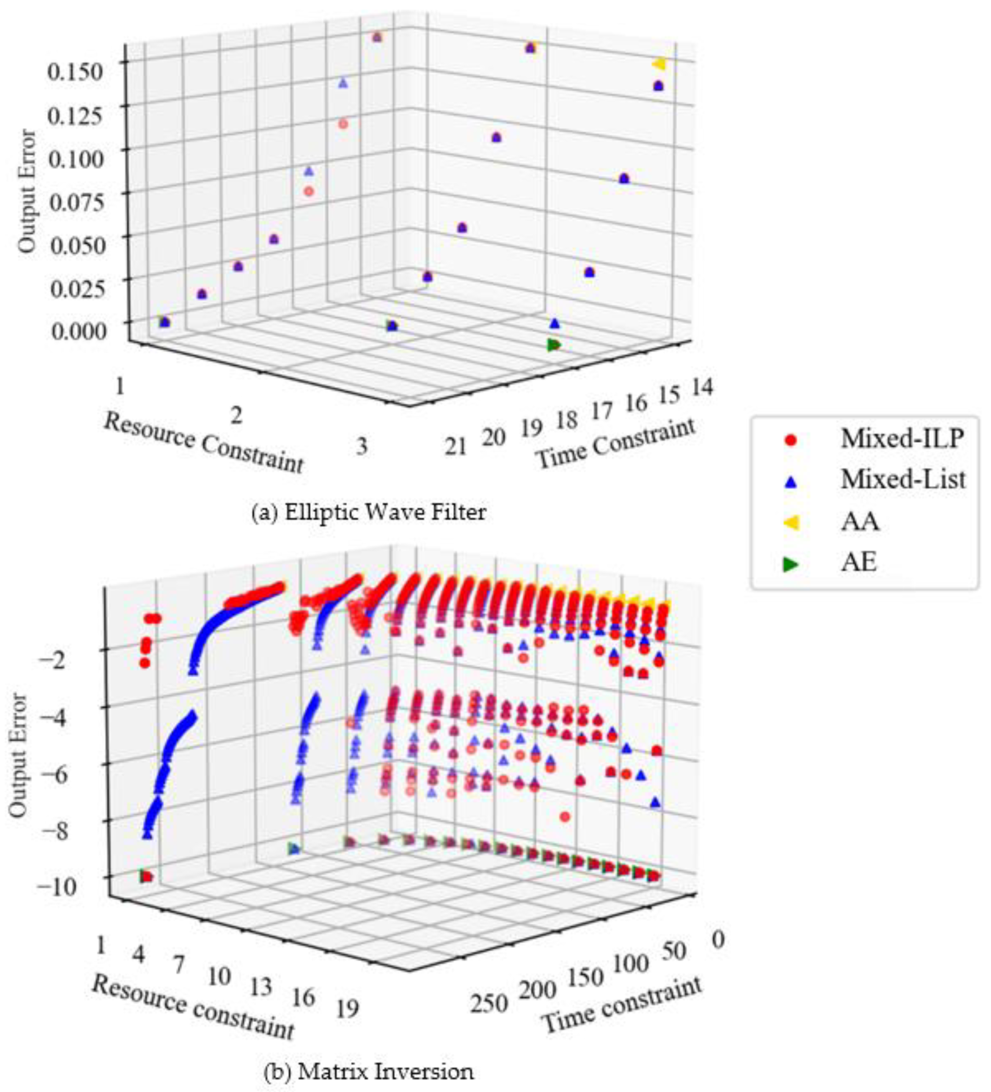
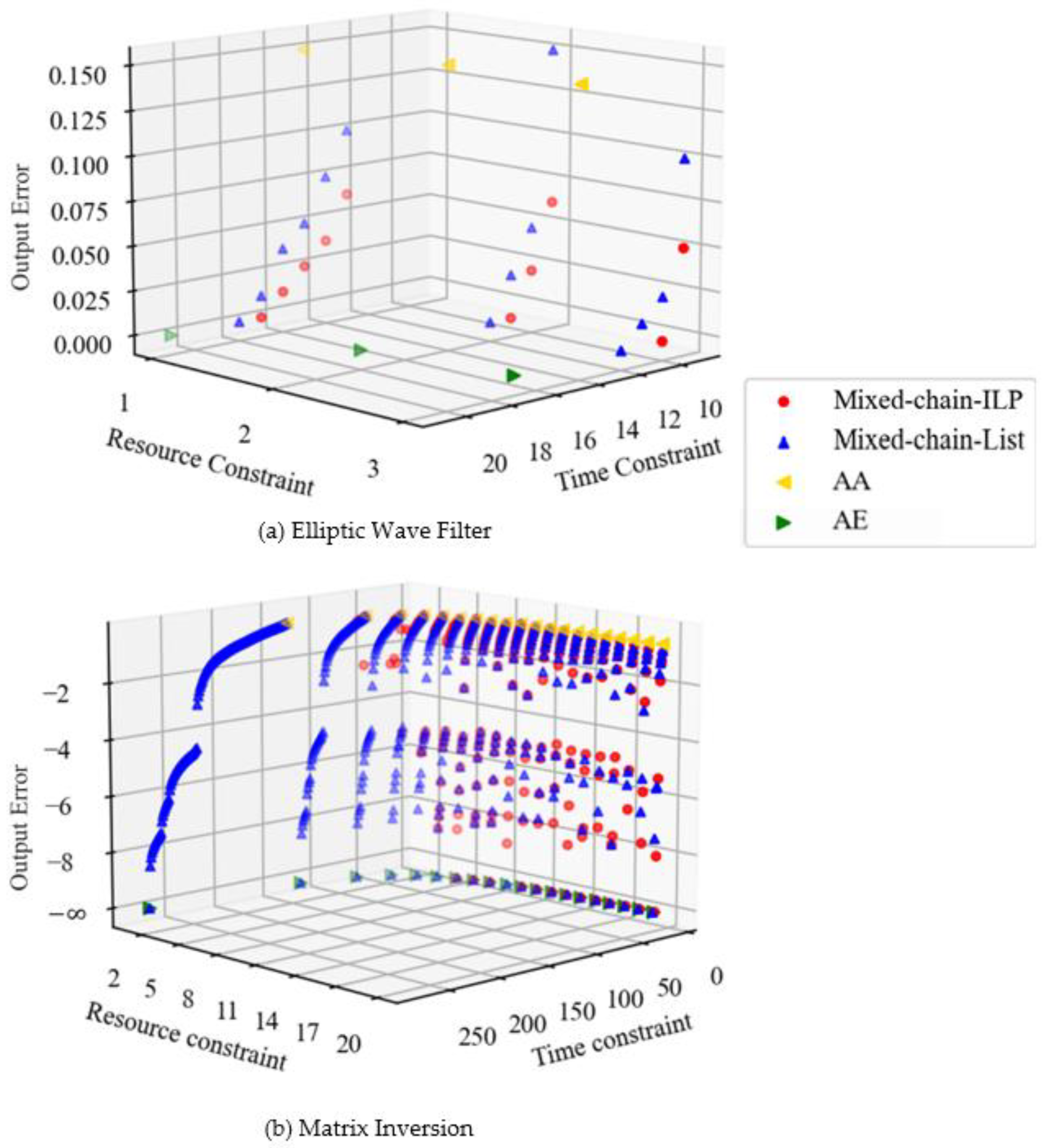
Figure 4 shows the scheduling results for each benchmark. The output error is denoted as the relative value of the error included in the output for the exact result. In Figure 4b, the output error is shown in logarithmic terms and is denoted as $-\infty$ when all multiplications are performed in two cycles (i.e., when there is no error). The higher the point, the more stringent the time constraint. The fewer the number of functional units that are constraints of the resource, the larger the difference between the number of cycles required to perform all the multiplications in one cycle and in two cycles. The scheduling results with a wide distribution of errors provide more options for circuit design. Because of this, it possible to find a solution that meets the designer’s requirements based on the area, execution time, and output error.

The Elliptic Wave Filter is regular and poses a short critical path of DFG compared to Matrix Inversion. Therefore, when the time constraint is increased and the number of approximate multiplications is reduced, the error of Mixed decreases slowly, as shown in Figure 4a. By comparison, Matrix Inversion is a complex DFG. In such a case, the magnitude of the error differs greatly depending on which multiplication is approximated. In Matrix Inversion, there is a multiplication on the critical path that has a large impact on the output error. Therefore, the distribution of the graph becomes narrower when the resource constraint is increased and the execution time is short. AA and AE in Figure 4 do not take error into account, and there is a trade-off between area and execution time. By comparison, Mixed minimizes the output error due to resource and time constraints, and a trade-off is established between area, execution time, and output error.

Table 2. Comparison of the list-scheduling solution with the ILP solution.

Benchmarks	Nodes (Mult)	Designs	Wins	Losses	Draws	ILP Exceeding 1 h
HAL	11 (6)	14	0	0	14	0
FIR filter	21 (11)	19	0	0	19	0
Auto Regression Filter	28 (16)	36	0	0	36	0
Motion Vectors Decoder	32 (14)	37	0	15	22	0
Elliptic Wave Filter	34 (8)	16	0	3	13	0
Cosine	42 (14)	52	0	1	51	0
Feedback Points	53 (17)	43	0	10	33	1
Matrix Multiplication	109 (40)	129	1	20	108	4
Smooth Triangle	197 (69)	257	35	63	159	55
Matrix Inversion	333 (140)	516	235	104	177	257

shows the comparison between list-scheduling algorithm and the ILP-based technique. In the table, Nodes represents the total number of operations for each benchmark. Mult means the number of multiplications among them. Designs indicates the number of design problems for a variety of resource and time constraints. Wins, Losses, and Draws represent the number of designs of our proposed algorithm that outperform the ILP-based technique in terms of accuracy, even slightly; the number of designs of the ILP-based technique that outperform our proposed algorithm; and the number where the same solutions are found, respectively. The number of times it takes more than one hour for ILP indicates the number of times the optimal solution is not obtained with ILP. In the Elliptic Wave Filter, there are three cases where the approximate solution for list scheduling is inferior to the optimal solution for ILP, but all the results in Figure 4a are close to the optimal solution. In Matrix Inversion, about half of the ILPs are not able to find the optimal solution in one hour. Most have no solution or a solution that is far from optimal and is inferior to the approximate solution of list scheduling. In contrast, list scheduling obtained solutions with a wide distribution regardless of the number of nodes. It can be said to be effective even for large applications.

Table 3. Runtime for scheduling (s).

Benchmarks	ILP			List Scheduling
	Max	Min	Mean	Max	Min	Mean
HAL	0.130	0.010	0.083	0.006	0.005	0.006
FIR filter	0.860	0.080	0.214	0.020	0.013	0.017
Auto Regression Filter	8.730	0.080	0.899	0.049	0.023	0.037
Motion Vectors Decoder	35.380	0.080	1.269	0.050	0.024	0.036
Elliptic Wave Filter	0.220	0.050	0.127	0.033	0.029	0.031
Cosine	2387	0.050	46.490	0.087	0.039	0.058
Feedback Points	>3600	0.080	85.617	0.138	0.066	0.100
Matrix Multiplication	>3600	0.200	149.748	2.044	0.527	1.092
Smooth Triangle	>3600	0.300	1155	15.804	2.865	7.204
Matrix Inversion	>3600	1.020	2116	170.288	16.217	70.913

shows the longest, shortest, and mean runtimes required for scheduling for each benchmark. ILP was unable to find an optimal solution in one hour when the number of nodes exceeded 50. However, list scheduling was able to find an approximate solution within three minutes even when the number of nodes exceeded 300. With ILP, scheduling can already take a long time for Cosine with 42 nodes; thus, if the number of nodes exceeds 300, it is expected to take several days to a month or more. As the number of nodes increases, the runtime increases exponentially, making ILP impractical. With list scheduling, there is a difference between the longest and shortest runtime with Matrix Inversion, which has a wide range of given time constraints. It is possible to obtain a near-optimal solution in a short time.

Table 4. Comparison of synthesized auto regression filter.

	AE (12 Cycle)	Mixed-ILP (12 Cycle)	Mixed-List (12 Cycle)
LUT	2686	2126	2228
FF	612	582	518
DSP	16	12	12
PSNR	$\infty$)	94.57	94.44
Power (uW)	29,189	25,924	27,777

shows the logic synthesis results of some of the scheduling results in Auto Regression Filter using Vivado 2020.1 on the xc7z020clg484-1 device. In the conventional method, we synthesized a circuit with AE performing in 12 cycles. In ILP and list scheduling, we synthesize Mixed circuits performing in 12 cycles. In these circuits, the performance of the circuit (number of cycles) was scheduled with the same constraints. Circuits designed with the two proposed methods both achieved low area and power by approximation. Furthermore, it is clear from the PSNR values that the magnitude of the error is minute. Therefore, the proposed method can design circuits with the same performance as that of the conventional method, having a low area and low power, without much loss of accuracy. Comparison of the PSNR of the proposed method shows that the approximate solution of list scheduling is almost equal to the optimal solution of ILP. The difference in area and power between the proposed methods, despite their equal accuracy, can be attributed mainly to the optimization of synthesis tools.

Figure 5 shows the scheduling results when chaining is considered. AA and AE here do not have chaining and are plotted at the same locations as in Figure 4. Comparing Figure 4a and Figure 5a, the execution time has been reduced and the error has been reduced. This is due to the fact that they are not only adding, but also chaining exact multiplication and addition. Comparing Figure 4b and Figure 5b, we can see that the results are similar to those of the Elliptic Wave Filter. Moreover, in the case of chaining, a wide distribution in terms of error is obtained even when resource constraints are large.

Table 5. Comparison of the list-scheduling solution with the ILP solution with chaining.

Benchmarks	Nodes (Mult)	Designs	Wins	Losses	Draws	ILP Exceeding 1 h
HAL	11 (6)	13	0	7	6	0
FIR filter	21 (11)	22	0	3	19	0
Auto Regression Filter	28 (16)	36	0	3	33	0
Motion Vectors Decoder	32 (14)	34	0	31	3	0
Elliptic Wave Filter	34 (8)	10	0	10	0	0
Cosine	42 (14)	47	0	35	12	0
Feedback Points	53 (17)	44	0	2	42	2
Matrix Multiplication	109 (40)	124	3	111	10	4
Smooth Triangle	197 (69)	248	35	91	122	61
Matrix Inversion	333 (140)	518	235	105	178	321

shows the results of comparing the list-scheduling solution with the ILP solution in terms of output error for each benchmark and summarizes the results, as shown in Figure 5. Compared to Table 1, there was no significant increase in the number of times the ILP exceeded one hour. The number of times the approximate solution for list scheduling is inferior to the optimal solution for ILP has increased. This is because the approximate algorithm does not perform chaining as effectively as ILP. However, as the number of nodes increases, the number of times that list scheduling outperforms ILP increases, indicating that the approximate algorithm is more effective for large-scale applications.

Table 6. Runtime for scheduling with chaining (s).

Benchmarks	ILP			List Scheduling
	Max	Min	Mean	Max	Min	Mean
HAL	0.140	0.050	0.083	0.014	0.008	0.010
FIR filter	17.530	0.090	1.141	0.044	0.020	0.032
Auto Regression Filter	60.840	0.090	3.220	0.115	0.039	0.079
Motion Vectors Decoder	43.250	0.130	2.071	0.117	0.039	0.073
Elliptic Wave Filter	0.530	0.160	0.049	0.058	0.042	0.380
Cosine	1675	0.090	38.162	0.192	0.078	0.115
Feedback Points	>3600	0.110	161.273	0.291	0.116	0.188
Matrix Multiplication	>3600	0.630	448.173	4.266	0.791	2.162
Smooth Triangle	>3600	0.360	1273	30.939	4.555	13.714
Matrix Inversion	>3600	8.750	2418	327.881	24.718	132.795

shows the longest and shortest runtimes required for chaining considered scheduling for each benchmark. In ILP, the runtime does not increase that much even when chaining is taken into account. In list scheduling, the runtime is approximately doubled by chaining. This is simply due to the increase in processing. However, list scheduling can still be solved in polynomial time.

The overall experimental results show that the proposed method can take advantage of approximate multipliers whose accuracy can be dynamically controlled in high-level synthesis. Although conventional scheduling explores circuits that meet the requirements through the trade-off between resource and performance, the proposed method incorporates approximate computing searches for circuits that meet requirements that are lower than those of the trade-off between resource, performance, and accuracy. Due to its flexibility, high-level synthesis can identify a more efficient circuit suitable for an application.

Our proposed ILP and list-scheduling methods have different characteristics in target applications. Although the ILP method can obtain an optimal schedule, the computational time becomes very long with the increase in the number of operations in applications. In contrast, the list-scheduling method can quickly find a circuit schedule while it sometimes fails to obtain an optimal schedule. In summary, the ILP method is preferred for use in a large application, and the list-scheduling method is suitable for a small application. In addition, we considered an optimization technique in high-level synthesis, and the two proposed methods show its practicality by chaining.

The circuit synthesis results show that the proposed method achieves lower power and lower cost with the same performance by applying approximations. Furthermore, it can be said that both the ILP and list-scheduling methods have small errors, although approximations are applied. This means that the proposed method improves resource and power use without much impact on the application. However, there is a large difference in power and resources used between list scheduling and ILP, even though the accuracy is almost the same. This indicates that it is necessary to consider memory resources and other factors when scheduling, and this is one of the issues to be addressed in the future. In addition, this research can be applied to ASICs. However, since we only experimented with FPGAs, this is also an issue to be addressed in the future.

6. Conclusions

We present a scheduling algorithm that exploits the difference in latency between approximate and exact operations in variable-cycle multiplication. The two proposed methods efficiently utilize approximate functional units whose accuracy can be dynamically controlled. The first method uses ILP to search for the optimal solution over time. The second method searches for a good solution in a short time by list scheduling. The two proposed methods extend the design search space compared to the conventional methods. This enables the design of approximate computing circuits that meet the requirements of resources, performance, and accuracy. The synthesized circuits based on the proposed method consumer less power and resources than conventional accurate circuits at the expense of small errors. In addition, they can be combined with optimization techniques and are practical. Although this paper focuses on approximate multipliers, the presented approach can be combined with other approximate methods.

Future studies will combine the presented approach with other optimization techniques such as pipelining and bitwidth reduction. In addition, since experiments were conducted only on FPGAs, we believe that experiments on ASICs will be necessary.

References

- Mittal, S. A survey of techniques for approximate computing. ACM Comput. Surv. 2016, 48, 1–33. [Google Scholar] [CrossRef]
- Xu, Q.; Mytkowicz, T.; Kim, N.S. Approximate computing: A survey. IEEE Des. Test 2016, 33, 8–22. [Google Scholar] [CrossRef]
- Jie, H.; Orshansky, M. Approximate computing: An emerging paradigm for energy-efficient design. In Proceedings of the 2013 18th IEEE European Test Symposium (ETS), Avignon, France, 27–30 May 2013. [Google Scholar]
- Ye, R.; Wang, T.; Yuan, F.; Kumar, R.; Xu, Q. On reconfiguration-oriented approximate adder design and its application. In Proceedings of the 2013 IEEE/ACM International Conference on Computer-Aided Design (ICCAD), San Jose, CA, USA, 18–21 November 2013. [Google Scholar]
- Camus, V.; Schlachter, J.; Enz, C. A low-power carry cut-back approximate adder with fixed-point implementation and floating-point precision. In Proceedings of the IEEE/ACM Design Automation Conference, Austin, TX, USA, 5–9 June 2016. [Google Scholar]
- Guputa, V.; Mohapatra, D.; Raghnathan, A.; Roy, K. Low-power digital signall processing using approximate adders. IEEE Trans. Comput.-Aided Des. Integr. Circxuits Syst. 2013, 32, 124–137. [Google Scholar] [CrossRef]
- Pashaeifar, M.; Kamal, M.; Kusha, A.A.; Pedram, M. Appproximate reverse carry propagate adder for energy-efficient dsp applications. IEEE Trans. Very Large Scale Integr. Syst. 2018, 26, 2530–2541. [Google Scholar] [CrossRef]
- Yang, T.; Ukezono, T.; Sato, T. A low-power configurable adder for approximate applications. In Proceedings of the 2018 19th International Symposium on Quality Electronic Design (ISQED), Santa Clara, CA, USA, 13–14 March 2018. [Google Scholar]
- Mahdiani, H.R.; Ahmadi, A.; Fakhraie, S.M.; Lucas, C. Bio-Inspired imprecise computational blocks for efficient VLSI implementation of Soft-computing applications. IEEE Trans. Circuits Syst. I Regul. Pap. 2010, 57, 850–862. [Google Scholar] [CrossRef]
- Lin, C.H.; Lin, I.C. High accuracy approximate multiplier with error correction. In Proceedings of the 2013 IEEE 31st International Conference on Computer Design (ICCD), Asheville, NC, USA, 6–9 October 2013. [Google Scholar]
- Liu, C.; Han, J.; Lombardi, F. A low-power, high-performance approximate multiplier with configurable partial error recovery. In Proceedings of the 2014 Design, Automation & Test in Europe Conference & Exhibition (DATE), Dresden, Germany, 24–28 March 2014. [Google Scholar]
- Yang, T.; Ukezono, T.; Sato, T. A low-power high-speed accuracy-controllable approximate multiplier design. In Proceedings of the 2018 23rd Asia and South Pacific Design Automation Conference (ASP-DAC), Jeju, Korea, 22–25 January 2018. [Google Scholar]
- Sano, M.; Nishikawa, H.; Kong, X.; Tomiyama, H.; Ukezoko, T. Design of a 32-bit accuracy-controllable approximate multiplier for FPGAs. In Proceedings of the 2021 18th International SoC Design Conference (ISOCC), Jeju, Korea, 6–9 October 2021. [Google Scholar]
- Nepal, K.; Li, Y.; Bahar, R.I.; Reda, S. ABACUS: A technique for automated behavioral synthesis of approximate computing circuits. In Proceedings of the Design, Automation & Test in Europe Conference & Exhibition, Dresden, Germany, 24–28 March 2014. [Google Scholar]
- Nepal, K.; Hashemi, S.; Tann, H.; Bahar, R.I.; Reda, S. Automated high-level generation of low-power approximate computing circuits. IEEE Trans. Emerg. Top. Comput. 2019, 7, 18–30. [Google Scholar] [CrossRef]
- Schafer, B.C. Enabling high-level synthesis resource sharing design space exploration in FPGAs through automatic internal bitwidth adjustments. IEEE Trans. Comput.-Aided Des. Integr. Circuits Syst. 2017, 36, 97–105. [Google Scholar] [CrossRef]
- Lee, S.; John, L.K.; Gerstlauer, A. High-level synthesis of approximate hardware under joint precision and voltage scaling. In Proceedings of the Design, Automation & Test in Europe Conference & Exhibition (DATE), Lausanne, Switzerland, 27–31 March 2017. [Google Scholar]
- Vaverka, F.; Hrbacek, R.; Sekanina, L. Evolving component library for approximate high level synthesis. In Proceedings of the 2016 IEEE Symposium Series on Computational Intelligence (SSCI), Athens, Greece, 6–9 December 2016. [Google Scholar]
- Venkatesan, R.; Agarwal, A.; Roy, K.; Raghunathan, A. MACACO: Modeling and analysis of circuits for approximate computing. In Proceedings of the 2011 IEEE/ACM International Conference on Computer-Aided Design (ICCAD), San Jose, CA, USA, 7–10 November 2011. [Google Scholar]
- Chan, W.T.J.; Kahng, A.B.; Kang, S.; Kumar, R.; Sartori, J. Statistical analysis and modeling for error composition in approximate computation circuits. In Proceedings of the 2013 IEEE 31st International Conference on Computer Design (ICCD), Asheville, NC, USA, 6–9 October 2013. [Google Scholar]
- Li, C.; Luo, W.; Sapatnekar, S.S.; Hu, J. Joint precision optimization and high-level synthesis for approximate computing. In Proceedings of the 2015 52nd ACM/EDAC/IEEE Design Automation Conference (DAC), San Francisco, CA, USA, 8–12 June 2015. [Google Scholar]
- Godínez, J.C.; Esser, S.; Shafique, M.; Pagani, S.; Henkel, J. Compiler-driven error analysis for designing approximate accelerators. In Proceedings of the 2018 Design, Automation & Test in Europe Conference & Exhibition (DATE), Dresden, Germany, 19–23 March 2018. [Google Scholar]
- Godínez, J.C.; Vargas, J.M.; Shafique, M.; Henkel, J. AxHLS: Design space exploration and high-level synthesis of approximate accelerators using approximate functional units and analytical models. In Proceedings of the 2020 IEEE/ACM International Conference on Computer Aided Design (ICCAD), San Diego, CA, USA, 2–5 November 2020. [Google Scholar]
- Xu, S.; Schafer, B.C. Exposing approximate computing optimizations at different levels: From behavioral to gate-level. IEEE Trans. Very Large Scale Integr. Syst. 2017, 25, 3077–3088. [Google Scholar] [CrossRef]
- Leipnitz, M.T.; Nazar, G.L. High-level synthesis of resource-oriented approximate designs for FPGAs. In Proceedings of the Design Automation Conference, Las Vegas, NV, USA, 2–6 June 2019. [Google Scholar]
- Leipnitz, M.T.; Nazar, G.L. High-level synthesis of approximate designs under real-time constraints. ACM Trans. Embed. Comput. Syst. 2019, 18, 59. [Google Scholar] [CrossRef]
- Leipnitz, M.T.; Perleberg, M.R.; Porto, M.S.; Nazar, G.L. Enhancing Real-Time Motion Estimation through Approximate High-Level Synthesis. In Proceedings of the 2020 IEEE Computer Society Annual Symposium on VLSI (ISVLSI), Limassol, Cyprus, 6–8 July 2020. [Google Scholar]
- Leipnitz, M.T.; Nazar, G.L. “Throughput-oriented spatio-temporal optimization in approximate high-level synthesis. In Proceedings of the 2020 IEEE 38th International Conference on Computer Design (ICCD), Hartford, CT, USA, 18–21 October 2020. [Google Scholar]
- Shirane, K.; Nishikawa, H.; Kong, X.; Tomiyama, H. High-level synthesis of approximate computing circuits with dual accuracy modes. In Proceedings of the 2021 18th International SoC Design Conference (ISOCC), Jeju, Korea, 6–9 October 2021. [Google Scholar]
- Shin, W.K.; Liu, J.W.S. Algorithms for scheduling imprecise computations with timing constraints to minimize maximum error. IEEE Trans. Comput. 1995, 44, 466–471. [Google Scholar]
- Lee, C.; Potkonjak, M.; Smith, W.H.M. MediaBench: A tool for evaluating and synthesizing multimedia and communications systems. In Proceedings of the 30th Annual International Symposium on Microarchitecture, Research Triangle Park, NC, USA, 3 December 1997. [Google Scholar]
Figure 1.
An example of scheduling for approximate computing circuits with variable-cycle approximate multipliers. (a) Approximate multiplications. (b) Exact multiplications. (c) Variable-cycle multiplications.
Figure 2.
Example of chaining in this work. (a) Add to Add (no Chaining). (b) Add to Add (Chaining). (c) Exact Mult to Add (no Chaining). (d) Exact Mult to Add (Chaining).
Figure 3.
Proposed list-scheduling example. (a) A given DFG. (b) Approximate all multiplications (result of first list scheduling). (c) Exact multiplication with the largest error(result of second list scheduling). (d) Exact multiplication with the second largest error (result of third list scheduling). (e) Exact multiplication with the smallest error (result of fourth list scheduling). (f) Final output that satisfies resource and time constraints.
Figure 4.
Comparison of ILP and list-scheduling errors.
Figure 5.
Comparison of ILP and list-scheduling errors with chaining.