
A CNN-GRU Approach to the Accurate Prediction of Batteries’ Remaining Useful Life from Charging Profiles


1
Department of Electronic Engineering, Institute of Information Science & Technology, Jeju National University, Jeju 63243, Republic of Korea
2
Department of Computer Engineering, Major of Electronic Engineering, Institute of Information Science & Technology, Jeju National University, Jeju 63243, Republic of Korea
*
Author to whom correspondence should be addressed.
Computers 2023, 12(11), 219; https://doi.org/10.3390/computers12110219
Submission received: 25 September 2023
/
Revised: 23 October 2023
/
Accepted: 25 October 2023
/
Published: 27 October 2023
Abstract
:Predicting the remaining useful life (RUL) is a pivotal step in ensuring the reliability of lithium-ion batteries (LIBs). In order to enhance the precision and stability of battery RUL prediction, this study introduces an innovative hybrid deep learning model that seamlessly integrates convolutional neural network (CNN) and gated recurrent unit (GRU) architectures. Our primary goal is to significantly improve the accuracy of RUL predictions for LIBs. Our model excels in its predictive capabilities by skillfully extracting intricate features from a diverse array of data sources, including voltage (V), current (I), temperature (T), and capacity. Within this novel architectural design, parallel CNN layers are meticulously crafted to process each input feature individually. This approach enables the extraction of highly pertinent information from multi-channel charging profiles. We subjected our model to rigorous evaluations across three distinct scenarios to validate its effectiveness. When compared to LSTM, GRU, and CNN-LSTM models, our CNN-GRU model showcases a remarkable reduction in root mean square error, mean square error, mean absolute error, and mean absolute percentage error. These results affirm the superior predictive capabilities of our CNN-GRU model, which effectively harnesses the strengths of both CNNs and GRU networks to achieve superior prediction accuracy. This study draws upon NASA data to underscore the outstanding predictive performance of the CNN-GRU model in estimating the RUL of LIBs.
1. Introduction
Lithium-ion batteries (LIBs) have garnered widespread adoption across various industries, including electric vehicles, portable electronics, the aerospace industry, submarines, and more. This is attributed to their remarkable advantages, including their increased energy density, elevated output voltage, minimal self-discharge, absence of memory effects, broad operational range, and eco-friendliness. Since their initial introduction, these advantages have firmly established LIBs as the preferred energy storage solution [1]. As the emphasis on environmental preservation continues to grow, many individuals are opting for energy-powered vehicles. When choosing such vehicles, two critical considerations come to the forefront: their range and safety features. However, it is essential to recognize that the chemistry of LIBs degrades over time, presenting a range of significant challenges [2]. Efficiently projecting the RUL of LIBs and providing preventive maintenance guidance to mitigate the risks associated with overcharging and discharging are imperative tasks. This critical endeavor is essential for upholding the security and dependability of the system and integrity of LIBs [3]. The reserve RUL estimates how old a battery is and how many cycles of charging and discharging it can withstand before failing in a given circumstance. Typically, a battery’s rated capacity is conservatively established between 70% to 80% of its failure threshold (FT) [4]. Prompt battery replacement becomes essential once the capacity reaches the FT. Failure to do so can result in LIB malfunction, jeopardizing energy storage equipment and even giving rise to catastrophic incidents [5]. Because battery capacity and RUL are closely correlated, most current RUL prediction techniques concentrate on predicting changes in LIB capacity. Enhancing the precision of RUL prediction for LIBs facilitates proactive maintenance approaches [6]. The degradation of a battery during a charge–discharge cycle is promptly evident through a reduction in battery capacity. To analyze battery performance deterioration and predict the RUL of LIBs, capacity is a direct indicator of health. The RUL can be described as follows in Equation (1):
The term “total available cycles” refers to a predefined number of charge–discharge cycles that a battery can endure, while the current cycle represents the ongoing charge–discharge cycle of the battery at a specific moment. Equation (1) calculates the remaining charge–discharge cycles that the battery can undergo before reaching its intended end of life. This calculation is based on the initial estimation of the total available cycles and the current usage [7]. The three main methods used to project the RUL of LIBs at this time are mechanism-based approaches, data-driven prediction techniques, and integrated prediction methodologies [8]. RUL prediction strategies are grounded in mechanism models such as the equivalent circuit process [9] and empirical degradation model method [10], which offer precise RUL forecasts under relatively stable external circumstances. However, these models’ accuracy can be susceptible to variations in external conditions. Employing historical feature data, the data-driven method of RUL prediction determines the correlations between battery characteristics and RUL. Techniques such as relevance vector machines (RVM)s [11] and neural networks (NNs) [12] belong to this category, and they have demonstrated remarkable flexibility and gained widespread adoption. A long short-term memory (LSTM) network optimized using an improved sparrow search algorithm (ISSA) was used to present a novel RUL prediction approach. Using the ISSA, hyperparameters that impacted prediction accuracy were tuned. Comparative tests revealed that the suggested process worked better than others, such as the SVR, CNN, RNN, and LSTM, thus enabling improved battery consumption [13].
A highly adaptable and resilient RUL prediction strategy was developed, and the method utilized multi-kernel RVMs that were optimized with the gray wolf optimizer to predict aging features for RUL prediction. In order to use complementary in ensemble empirical mode decomposition and, that the quantifiable and historical aging characteristics were split into high- and low-frequency signals. An LSTM NN and a feedforward neural network (FNN) were then used to model and forecast these signals with changing frequency, respectively [14]. The extensive utilization of deep-learning neural networks, particularly the LSTM NN, excels in accurately forecasting battery capacity and RUL, making it a valuable tool for measuring battery aging data. Its proficiency in storing and updating information over extended periods without encountering the vanishing gradient issue significantly contributes to its elevated prediction precision. Chinomona et al. [15] employed a forward-selection LSTM technique. The approach adeptly extracted an optimal feature subset from raw signals by filtering out irrelevant features. Park et al. [16] presented a many-to-one LSTM structure to correctly predict the RUL for LIBs. In their study, a data-driven ELM neural network model was employed to address the challenging task of predicting the RUL of LIBs. An ELM neural network was used for passive mapping to transform the problem into a high-dimensional space, and random input weights and thresholds were introduced [17]. The sliding time window technique was employed to process input data samples to capture valuable feature information from the input data and predict the RUL. These feature-rich data were then leveraged to make RUL predictions. Within the domain of RUL prediction, the LSTM NN, a notable improvement over traditional recurrent NNs, plays a pivotal role. In this context, the RUL prediction method developed by [18] is a noteworthy contribution.
Batteries are essential for many contemporary technologies, including electric cars, renewable energy sources, and portable electronics. Ensuring their reliable performance and longevity is paramount to the functionality and sustainability of these applications. Predicting the RUL of batteries has emerged as a critical challenge, as it allows for proactive maintenance and replacement strategies, ultimately reducing downtime and operational costs. Conventional RUL prediction methods have traditionally relied on statistical and physics-based models. While effective to some extent, these methods often struggle to capture the complex and nonlinear behaviors exhibited by batteries, particularly when confronted with diverse operational conditions and varying usage patterns. In this study, we address and confront two fundamental challenges. Firstly, our goal is to improve LIB RUL prediction accuracy. This goal unites researchers in the pursuit of the most precise results. Secondly, we grapple with the challenge of optimizing the overall execution time of our hybrid method. This process encompasses various tasks, including data extraction, formatting, model training, validation, and performance computation, all of which can be time-consuming. Given the complexity of our hybrid approach, it is essential to streamline these operations to achieve quicker and more efficient RUL predictions. These two issues serve as the foundation for our research, which aims to increase the accuracy and effectiveness of RUL prediction for LIBs.
We developed the CNN-GRU approach to address these challenges; this was designed to combine CNN and GRU architectures. In this study, we address the pressing need for more accurate predictions of the RUL of LIBs. These batteries play a crucial role in various industries, and ensuring their reliability and efficiency is paramount. However, existing methods have limitations in their ability to accurately estimate RUL. To overcome these limitations, we harness data-driven approaches, capitalizing on the power of machine learning techniques, which have gained increasing attention in recent years due to their potential to significantly enhance RUL predictions. Notably, the integration of deep learning architectures has brought about innovation in this field. Deep learning models, such as CNNs, have demonstrated remarkable capabilities in uncovering intricate data patterns and relationships, particularly in multi-dimensional data. This makes them exceptionally well suited for extracting crucial information from various battery parameters, including V, I, and T. Simultaneously, RNNs, including LSTM and GRU, have demonstrated their efficacy in simulating temporal relationships in sequential data. Our research presents a fresh and groundbreaking method for predicting battery RUL. We combine the best features of CNNs and GRUs into a hybrid architecture with the intention of drastically improving the precision and efficacy of RUL predictions. This innovative CNN-GRU hybrid model concurrently extracts spatial and temporal features from multi-channel charging profiles. While CNNs capture spatial information from V, I, and T data streams, the GRU model captures the time-dependent patterns associated with battery capacity. To validate the effectiveness of our method, we conducted extensive experiments using NASA’s battery datasets.
The main contributions of this article are summarized as follows:
- We introduce a hybrid deep learning model for accurate battery RUL prediction by combining CNN and GRU architectures.
- Our model utilizes the parallel processing of multiple measurable datasets (V, I, T, and capacity) with the CNN and GRU to extract relevant features.
- The CNN captures spatial information from multi-channel charging profiles, while the GRU focuses on time-dependent data derived from previous capacity profiles.
- Our extensive experiments demonstrate a significant improvement in precision for the estimation of the remaining charge and prediction of the RUL using our model.
- We provide a comparative analysis of our RUL prediction results with those from relevant studies in the literature.
The remainder of this paper is structured as follows: Section 2 delves into the related work concerning the RUL prediction model. Section 3 elaborates on the proposed methodology. We provide details about the dataset in Section 4, and Section 5 is dedicated to presenting experimental results and discussions. Lastly, we conclude the paper and outline potential future research directions.
2. Literature Review
In recent years, battery management and predictive maintenance have seen significant growth due to the escalating demand for efficient energy storage solutions across various applications. The accurate prediction of RUL is a pivotal component of effective battery management, and it has attracted substantial attention from academia and industry. This section extensively reviews existing RUL prediction methodologies while focusing on applying machine learning techniques to address this complex challenge.
2.1. RUL Definition
The RUL of LIBs is a fundamental metric in battery management and predictive maintenance. Its standard definition is the amount of time that passes between the present cycle and the battery’s end-of-life (EoL) stage. The EoL represents a critical point in a battery’s lifecycle, signifying the end of its reliable performance. Traditionally, the EoL is recognized when a battery’s capacity degrades to approximately 70% to 80% of its nominal capacity. This specific range of capacity degradation—often referred to as the “end-of-life threshold”—serves as a widely accepted parameter for characterizing the remaining lifespan of LIBs. Therefore, estimating a battery’s RUL is akin to determining the probability distribution function (PDF) when the battery’s capacity satisfies these well-established EoL criteria [19]. This definition of the EoL based on capacity degradation has been widely adopted in battery management [20,21]. The RUL is a valuable and concrete measure of a battery’s remaining usable life and an essential parameter for many applications, including electric vehicles and renewable energy storage. The accuracy of RUL predictions is vital for optimizing battery maintenance strategies, ensuring safety, and preventing unexpected failures in real-world scenarios.
2.2. RUL Prediction Methods and Strengths and Weaknesses of Existing Methodologies
The field of RUL prediction for batteries has experienced a significant transformation, moving away from conventional empirical techniques to embrace more advanced data-driven approaches. Early methodologies primarily relied on simple time-based degradation models, which had limited adaptability when confronted with battery degradation’s dynamic and nonlinear nature under varying operational conditions. However, recent advancements have introduced numerous techniques that harness the wealth of data collected during battery operation, significantly enhancing the accuracy of RUL predictions. The landscape of battery RUL prediction can be categorized into three key approaches: physics-based models, data-driven models, and hybrid models. Each approach possesses unique strengths and limitations, and their utilization depends on specific requirements. Physics-based models delve into the intricacies of battery processes, offering insights into the causes of degradation but requiring precise calibration. Data-driven models leverage extensive datasets, with both shallow and deep learning techniques contributing to enhanced prediction accuracy. Hybrid models merge the strengths of data-driven and mechanistic models, improving stability and precision. Predicting the RUL of LIBs is a complex task influenced by various factors, presenting opportunities for innovative research to enhance accuracy and address existing challenges [22]. RUL prediction plays a pivotal role in battery health management and assessing the value of retired batteries. In cascading utilization, estimating the RUL ensures timely replacement, preventing safety issues. Calculating a battery’s reserve life (RUL) is difficult because of the variety and complexity of the elements that affect it, including the battery’s health, past performance, and failure modes. RUL prediction methods can be broadly categorized into two main groups: data-driven and hybrid approaches, as shown in Figure 1.
The amalgamation approach involving data-driven and mechanistic models primarily entails the integration of mechanistic models guided by electrochemical principles and empirical mathematical models. As outlined in [23], in order to utilize this technique, the battery is subjected to a series of precise current excitations that are used to determine the parameters for a reduced electrochemical model. The particle filter (PF) method then utilizes these parameters as state variables to create an observation equation. In turn, the observation equation makes it easier to forecast the RUL for LIBs. Guha et al. [24] formulated an empirical model delineating the progression of internal resistance alongside a capacity degradation model that leveraged data extracted from EIS tests. The resultant model was harnessed within the PF framework to prognosticate the RUL of LIBs across distinct lifecycle phases. However, the advancement of this fusion prediction model is impeded by the challenges posed in constructing more intricate and precise mechanism models, along with issues such as excessive noise and particle depletion in predictions [25]. In [26], a new strategy was suggested to extend the lifespan of power conversion designs with modular connections, which are widely utilized in various power electronics applications. The approach employed a Levenberg–Marquardt backpropagation neural network (LM-BPNN) to estimate the system’s health without requiring complex mathematical models. It incorporated power routing, which allowed different power levels for cells based on their damage, thus delaying the failure of highly damaged cells. Numerical simulations confirmed the effectiveness of this approach in prolonging the system’s overall lifespan. The method was experimentally verified with an interleaved DC–DC boost conversion setup.
These difficulties similarly constrain the performance of the forecast. Numerous data-driven fusion strategies have attracted much interest and support in RUL prediction. Interestingly, deep and shallow machine learning methods often employ data-driven methodologies. An artificial bee colony (ABC) was used in the RUL prediction approach of Wang et al. [27] to optimize support vector regression (SVR) kernel parameters. This method successfully resolved the difficulty of figuring out the SVR kernel settings. Cai et al. [28] pioneered the utilization of the artificial fish swarm algorithm (AFSA) to fine-tune the kernel parameters of the RVM. They subsequently employed a discrete gray model to project trends, effectively amalgamating the nonlinear regression capabilities of the relevance vector machine. Through this comprehensive approach, the prediction of the RUL for LIBs was successfully achieved. A fusion method that combined SVR and PF was used in [29] to forecast the RUL for LIBs. Interestingly, the common practice in these approaches was to combine an optimization algorithm with a single data-driven algorithm to predict the RUL. This methodology is rooted in the intrinsic instability of prediction results due to uncertainty around important parameters in various single data-driven algorithms. As a result, combining data-driven algorithms with optimization approaches has become a standard method of improving the predictive stability of models. In [30,31], it has introduced an innovative approach based on Support Vector Machines (SVM) for predicting the RUL of LIBs. The method has attained precise real-time RUL predictions by extracting pivotal features from the battery data. Several methods have demonstrated success in predicting RUL for LIBs. For instance, SVR optimization techniques, such as the ABC algorithm, have proven effective in optimizing kernel parameters. Additionally, models like the RVM have been employed alongside optimization algorithms to enhance predictive accuracy. These algorithms excel in handling intricate patterns and nonlinear correlations within battery data. Deep learning—particularly with LSTM networks and hybrid neural networks—has emerged as a standout choice for modeling RUL prediction. LSTM, with its capability of capturing temporal dependencies, is well suited for handling the complex patterns observed in LIBs.
2.3. The RUL Based on Machine Learning Models
Due to their ability to recognize intricate patterns and nonlinear correlations in battery data, ANNs have become renowned as versatile and effective methods for RUL prediction. ANNs assess incoming data and generate predictions through organized networks of interconnected nodes or neurons. One of their primary advantages is the ability to handle multivariate time-series data, including voltage, current, temperature, and impedance measurements. Their architecture enables them to capture temporal dependencies and dynamic patterns in battery operation, ultimately contributing to more accurate RUL predictions. Several ANN architectures have been explored for RUL prediction, including feedforward networks, recurrent networks, and hybrid models that combine different neural layers. Additionally, ensemble techniques and regularization methods have been integrated to enhance ANN models’ robustness and generalization capabilities. In the realm of deep learning, RNNs are prevalent, with LSTM algorithms being a standout choice. LSTM’s proficiency in modeling sequences and capturing temporal dependencies makes it well-suited for predicting the RUL in domains such as LIBs. The architecture’s ability to retain and utilize historical information over extended sequences addresses challenges such as vanishing gradients, which are crucial for understanding battery degradation patterns. LSTM’s versatility in capturing short-term fluctuations and long-term trends contributes to accurate RUL predictions for optimizing resource utilization and maintenance strategies [32,33].
In [34], a dynamic LSTM approach that enabled online RUL prediction was introduced. Notably, health index creation relied on indirect voltage measures instead of battery capacity. In [35], an ensemble strategy incorporating LSTM was proposed, accounting for uncertainty through Bayesian model averaging. Furthermore, the authors of [36] merged LSTM with particle swarm optimization and enhanced LSTM parameters that were computed by aligning with the designated topology. LSTM excels at modeling sequences that are suitable for battery performance time series. Hybrid NNs combine these strengths, yielding accurate RUL predictions by leveraging various network structures, as NNs have enhanced RUL prediction accuracy and handle intricate LIB behaviors effectively [37]. The authors of [38] introduced an enhanced variant of the LSTM neural network, demonstrating heightened information extraction capabilities. Wang et al. [39] employed an enhanced RVM approach that considered inevitable uncertainties and integrated expectation–maximization (EM) for model refinement. Despite the advantageous trait of requiring minimal training data, both the SVM and RVM face challenges of diminished prediction accuracy due to significant sparsity and limitations in addressing time-series issues. In the realm of predicting the RUL for LIBs, NN methods have played a crucial role. Approaches such as the extreme learning machine (ELM), LSTM, GRU, and hybrid NNs have been widely utilized. The ELM stands out due to its efficient training and adaptability to diverse architectures. This versatile method has undergone innovative adaptations to enhance its applicability. These adaptations target the elimination of the need to predefine neuron counts and hidden layer weights, catering to the diverse demands of battery RUL prediction.
Notable among these adaptations is the kernel ELM (KELM) [40,41], which introduces a kernel-based approach in order to augment the ELM’s capabilities, enabling it to tackle complex patterns in battery data. Additionally, the emergence of the multiple-kernel ELM (MKELM) [42] signifies a stride towards accommodating varying data representations, thus contributing to the refinement of RUL estimates. This study introduced a new model for predicting the RUL of batteries named the particle filter–temporal attention mechanism–bidirectional gated recurrent unit (PF-BiGRU-TSAM). The model added importance to battery capacity at different time points by combining an offline-trained BiGRU-TSAM with historical data training. The advantages of both model-based and data-driven models were combined and allowed to complement one another throughout the online prediction phase [43]. The expectation–maximization–unscented particle filter–Wilcoxon (EM-UPF-W) approach was developed in this study to properly detect capacity regeneration and estimate noise factors in battery deterioration models. To be more precise, the method produced a dynamic deterioration model for individual batteries that had been exposed to UPF. Additionally, the EM technique was used to adaptively estimate noise variables, especially when a few samples were without labels. Furthermore, the Wilcoxon rank sum test was presented in order to determine the capacity regeneration point and, eventually, reduce forecast errors [44]. A comprehensive comparative analysis of diverse model-based techniques for the prediction of the RUL has been presented, and valuable insights into their strengths and advantages are offered in Table 1.
3. Methodology
In this section, we present our innovative methodology for precise RUL prediction in LIBs. Our approach consists of a carefully structured process designed to maximize prediction accuracy and robustness. The first phase of our methodology begins with rigorous data preprocessing to ensure the quality of the input data. This phase addresses data anomalies, removes outliers, handles missing values, and normalizes the dataset. The second phase involves selecting input features, including voltage (V), I, T, and capacity. These choices are rooted in their fundamental significance for battery behavior. Voltage is a vital indicator of electrochemical reactions within the battery, reflecting variations in energy output. Current, representing the flow of energy, plays an essential role in understanding the dynamic state of a battery. Temperature, another crucial factor, directly impacts a battery’s aging process, influencing its overall health. Lastly, capacity characterizes a battery’s energy storage capabilities and its ability to maintain charge. In the third step, our methodology leverages a hybrid model combining a CNN and GRU. This decision was made because it is necessary to record temporal and geographical relationships in the battery data. Parallel CNN branches are used for each input feature (V, I, T) to capture spatial information independently.
Simultaneously, a GRU layer models the temporal dependencies in capacity data, which are inherently related to time-dependent behavior. The fourth phase divides the preprocessed data into training, validation, and testing sets. This division ensures that the model is effectively trained on historical data, validated for robustness, and rigorously tested for predictive accuracy. The selected model architecture is fine-tuned and trained using preprocessed data during training. This process enables the models to capture intricate patterns in battery behavior, further enhancing the predictive capabilities. Our trained models estimate and evaluate the battery’s RUL in the final phase. We evaluate the precision and dependability of our predictions using specialized error measures designed for RUL prediction tasks. The process begins with step 1, battery data, where essential information related to the batteries is gathered. In step 2, data preprocessing, this collected data undergoes cleaning and organization. In step 3, train model for RUL estimation, the preprocessed data is utilized to train a model capable of estimating the batteries’ remaining useful life (RUL). The final step, step 4, method evaluation, involves evaluating the model’s performance to determine its effectiveness in predicting battery life. These four steps provide a structured workflow for managing battery data and estimating RUL, as shown in Figure 2, which illustrates the overall framework of the proposed approach.
3.1. Theoretical Background of the Study
Before delving into the core of our study, it is essential to lay a strong theoretical foundation. In this section, we will elucidate the essential ideas and architectures that form the basis of our research. We will explore CNNs, LSTM, and GRUs. Additionally, we will present the proposed framework models, including their hybrid variations: CNN-LSTM and CNN-GRU.
3.1.1. Convolutional Neural Network Model
CNNs are a potent class of neural networks that are highly renowned for their proficiency in various deep-learning applications. They are a specific type of feedforward neural network (FNN). The architecture of CNNs comprises convolutional and pooling layers, which are particularly adept at extracting pertinent features from data. Subsequently, one or more fully connected layers come into play, and these features are leveraged to make predictions. During the training process, the CNN acquires the ability to correlate the extracted features with the appropriate labels. This achievement is unlocked through iterative mechanisms such as backpropagation and optimization [50,51]. A typical CNN comprises several essential layers, including the input, convolutional, pooling, fully connected, and output layers. These networks are widely used in various deep-learning tasks. CNNs are designed to operate on multi-dimensional input feature vectors. The convolutional layers play a crucial role in identifying intrinsic relationships within the data by extracting feature maps. These feature maps are then processed through pooling layers, which perform subsampling to reduce network complexity and prevent overfitting. The convolutional kernel operates on the width of the convolution development, further improving the extraction of relevant feature information. Finally, the fully connected layers integrate the processed data following the convolution and pooling stages. These merged data are subsequently fed into the final layers of the network, often including a fully connected or recurrent layer for making predictions, as shown in Figure 3, which is a basic CNN architecture.
Figure 2.
Workflow of the proposed approach.

3.1.2. LSTM Model
Due to the nature of the data collected from LIBs, which involve charging and discharging cycles and are essentially time-series data, using an RNN is a reasonable choice for processing such sequences while leveraging internal memory. RNNs are equipped with internal feedback and feedforward connections among their processing units, allowing them to handle sequential information. However, it is important to note that RNNs have limitations, particularly when dealing with long sequences. They can only store a portion of a sequence, which can lead to reduced accuracy when dealing with longer sequences [52]. In this context, where LIB data sequences are relatively lengthy and consist of numerous time series, LSTM networks are preferred over traditional RNNs. LSTM is a specialized type of RNN designed to overcome the challenge of handling long-distance dependencies in sequences. LSTM networks are particularly effective at capturing and learning from sequences with extended context, making them well-suited for tasks involving time dependencies. For instance, LSTM models can effectively model how a battery’s capacity changes over time during discharging profiles. One key feature of LSTM is its ability to maintain a certain level of correlation between hidden-layer nodes. When the network receives sequential data, the hidden-layer nodes’ computations rely on both the current input and the activation levels of the nodes from earlier time steps. When processing sequences that are input-related for LIBs, the LSTM network layer processes both the output and hidden-layer sequences. This allows it to efficiently identify intricate patterns and dependencies in the data. The input gate, forgetting gate, and output gate are the three gates that allow the LSTM to function. Together, these gates enable the data to write, read, and maintain long-term dependencies. Figure 4 depicts the layout of the LSTM abstraction network.
3.1.3. Gated Recurrent Unit Model
The development of RNNs—particularly LSTM networks—successfully addresses a critical issue faced by fully connected neural networks. The problem is that fully connected networks tend to experience data loss in either space or time, which results in challenges related to vanishing and exploding gradients. These two issues, known as vanishing and exploding gradients, were effectively resolved by introducing the concept of gates in the LSTM network. Input, output, and forgetting gates are components of an LSTM network that regulate and control information flow. This innovation allows LSTM to capture and learn from sequences with long-range dependencies, addressing the challenges associated with data loss. Another noteworthy advancement in this context is the GRU, which can be considered an enhanced version of the LSTM model. The GRU retains the training effectiveness of LSTM while streamlining the network’s topology and reducing the number of training parameters. This makes the GRU a more efficient choice for handling sequential data such as LIB charging and discharging profiles. A single step of the GRU update equations is shown in Figure 5; at the core of this architecture are two crucial gates: the update gate and the reset gate . These gates play pivotal roles in regulating information flow and capturing temporal dependencies within the data.
The update gate combines the functions of the forgetting and input gates in traditional recurrent networks. It determines what information to retain from the previous state and what new information to add. The formula for is shown in Equation (2):
where is the update gate at time step t in a GRU model that determines how much of the previous hidden state to retain and how much new information to incorporate . The activation function squeezes values between 0 and 1, controlling information flow. is the weight matrix for the update gate, and it influences the importance of input and the prior hidden state . is a concatenation of the current input and previous hidden state to form the update gate’s input. is a bias term that shifts the sigmoid’s decision boundary to fine-tune the gate’s behavior in Equation (2).
The reset gate, represented by , is another integral component of our architecture. When calculating the present state, it sets the amount of the prior condition that should be erased or reset. By modulating the memory resetting, allows the network to selectively keep or discard details from previous time steps and capture relevant patterns and dependencies in the data. The formula for is as follows:
where (the reset gate) defines how much of the last hidden state to reset or forget when computing the new hidden state at time step t based on the current input . The sigmoid activation function squashes the weighted sum of the input and previous hidden state, ensuring that takes values between 0 and 1, thus controlling the amount of reset involved in Equation (3).
3.1.4. CNN-LSTM Model
Our battery RUL prediction methodology uses a hybrid deep model that combines a CNN and an LSTM network in a data-driven manner. In order to extract characteristics from several quantifiable data sources, such as voltage, current, temperature, and capacity, these two components operate in parallel, as shown in Figure 6. The CNN focuses on extracting features from multi-channel charging profiles, while the LSTM specializes in capturing features from historical capacity data associated with discharging profiles while considering their time-dependent nature.
3.1.5. CNN-GRU Model
The CNN-GRU architecture is a powerful fusion of CNNs and GRUs that is meticulously designed for complex data analysis tasks. This hybrid model seamlessly combines the spatial feature extraction capabilities of CNNs with the temporal dependency modeling strengths of GRUs. In the context of battery RUL prediction, CNNs play a pivotal role in extracting essential spatial features from various input data sources, such as V, I, T, and capacity. These extracted features are then seamlessly integrated into the GRU layer, which excels in capturing temporal relationships and historical capacity data. The overall framework of the CNN-GRU model suggested in this research consists of four key layers: the input, CNN, GRU, and output layers. The process begins with the CNN layer, which extracts essential information related to lithium battery health factors by mining the natural correlations between feature quantities and lithium battery capacity. Following this, the pooling layer conducts computations by utilizing convolution kernels to extract additional feature data and broaden the scope of the convolution results. The preprocessed lithium battery data are then passed into the GRU network for optimization training through a fully connected layer. Within the GRU layer, the model learns the underlying patterns and internal variability, which are crucial for making accurate predictions. Finally, the output layer generates valuable predictions related to lithium battery capacity, providing valuable insights into the battery’s RUL. This comprehensive architecture enables accurate RUL predictions for LIBs to the benefit of various applications and industries. The hybrid RUL prediction model was constructed using a CNN-GRU channel attention mechanism, as shown in Figure 7.
4. Data Description
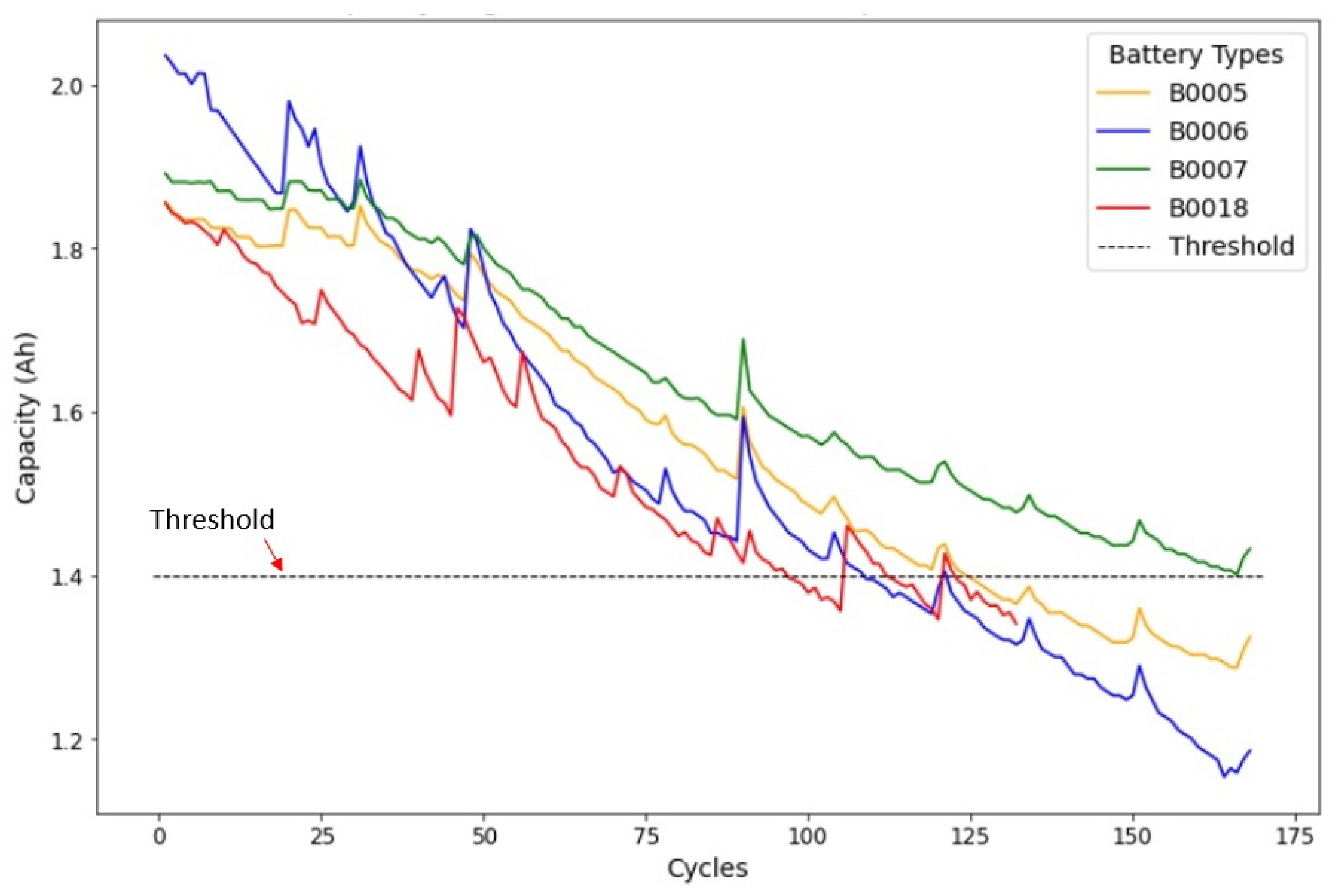
Our study commences with an introductory examination of the dataset in [53], which encompasses four LIBs, namely, B0005, B0006, B0007, and B0018. These batteries have undergone a series of charge, discharge, and impedance operations. The impedance analysis was conducted using electrochemical impedance spectroscopy (EIS) across varying frequencies. Consecutive charge and discharge cycles have led to the expedited aging of the batteries, and this aging process was reflected in the evolving internal battery parameters, as unveiled by the impedance measurements. The selection criteria were their initial state of health (SoH), capacity, and model name. There were two thorough steps in the billing procedure. The end-of-life (EoL) criterion was reached, which signified a 30% capacity decline from the initial rated capacity of 2 ampere-hours (Ahr) to 1.4 Ahr. At that point, the studies were terminated. These datasets hold valuable potential for forecasting the residual charge (within a designated discharge cycle) and the batteries’ RUL. This study’s dataset included aging data for 18,650 lithium cobalt oxide batteries with a 2 Ah capacity, which were generously provided by NASA. The analysis focused on the cycling behavior of four specific lithium batteries, and all analyses were conducted at room temperature. The results of this analysis unveiled the capacity decay curves for B0005, B0006, B0007, and B0018 at a temperature of 24 °C, as illustrated in Figure 8.
4.1. Charge, Discharge and Impedance Profiles
The charge profiles exhibited striking consistency across all battery tests, offering a clear window into the intricate behaviors of the system. The charging procedure was meticulously executed, commencing with a stable power input through a constant current (CC) mode, which was precisely set at 1.5 A. This phase persisted until the battery voltage reached its highest point, peaking at 4.2 V. A transition occurred, moving into a constant voltage (CV) mode. This mode was maintained until the charge current gently diminished to a mere 20 mA. In contrast, the discharge phase presented an array of diversity, with each battery showcasing its distinctive characteristics. The discharge process was meticulously regulated by a controlled CC regimen, spanning a range from 1 A to 4 A, which was tailored to the specific battery under investigation. This discharge process persisted until the battery voltage gracefully descended to well-defined thresholds: 2.7 V, 2.5 V, 2.2 V, and 2.5 V. These distinct thresholds illuminated the batteries’ unique resilience and performance attributes as they navigated the discharge process, offering insights into their behaviors across various energy levels. Furthermore, the impedance measurements furnished a multifaceted understanding of battery dynamics, transcending the boundaries of voltage and current.
The batteries’ internal responses came to life by deploying EIS across frequencies. These measurements uncovered intricate electrochemical processes and material behaviors within the battery systems. Impedance measurements were conducted using EIS with a frequency sweep spanning from 0.1 Hz to 5 kHz. The experiments were concluded when the batteries met specific EoL criteria. For instance, one criterion involved a 30% reduction in rated capacity, declining from 2 Ampere-hours (Ahr) to 1.4 Ahr. Additionally, alternative stopping criteria were employed, including a 20% reduction in a rated capacity. Table 2 presents a summary of the experimental specifications for the battery dataset, including the various charging, discharging, and impedance modes.
4.2. Data Preprocessing
Data preprocessing is essential for predicting the RUL of LIBs. This critical phase includes key techniques that enhance the quality of input data, directly impacting the RUL prediction accuracy. Handling missing values is crucial, as sensor-read gaps (V, I, T, capacity) can disrupt data continuity. Imputing missing values—often by using mean or median imputation methods—ensures data integrity and more precise predictions. Outliers represent extreme deviations or anomalies in the data, introducing unwanted noise during model training. Removing these outliers improves model performance and enables accurate pattern learning in LIB RUL prediction. Also, normalization is a critical step because LIB data come from diverse sensors with varying units and scales. Normalization standardizes these features to a consistent range (usually between 0 and 1), preventing any single feature from dominating the model’s learning process. This facilitates more efficient model convergence and enhances prediction accuracy.
5. Experimental Results and Discussion
This section is divided into three main components; the first part encompasses the evaluation criteria and system configuration of the RUL prediction model. The second part presents the prediction results and comprehensively discusses the RUL prediction model. Finally, the third part provides a summary of the suggested technique.
5.1. Evaluation Criteria and System Configuration
During the model training phase, the CNN network employs the same convolution technique while utilizing 8, 16, and 32 convolution kernels in three convolution layers and one pooling layer. Every battery dataset was first divided into testing and training sets, with a data split of 20% and 80%, respectively. Batteries were combined in many ways for testing, validation, and training, and three situations were employed in our investigation. For example, in scenario 1, battery B0006 and battery B0007 were used as a training set, while battery B0005 was employed for validation, and battery B0018 served as the testing set. Similarly, in scenario 2, battery B0005 and battery B0006 constituted the training sets, with battery B0007 being used for validation and battery B0018 being used as the testing set. This approach allowed the model’s performance to be comprehensively evaluated across different battery datasets and configurations, with the same process being followed for all battery data. To emphasize the comprehensive validation of the experiment, we employed the following four evaluation criteria to assess the CNN-GRU model’s performance in predicting the RUL.
In Equation (4), the mean absolute error (MAE), for which a lower value indicates superior prediction performance, is expressed as follows:
In Equation (5), the root mean square error (RMSE), for which a lower value signifies superior prediction performance, is expressed as follows:
In Equation (6), the mean absolute percentage error (MAPE) provides a meaningful way to assess prediction accuracy, particularly when understanding the relative error is crucial, and lower MAPE values indicate better prediction performance.
In Equation (7), the mean squared error (MSE) is valuable for assessing prediction accuracy and places a higher weight on more significant errors due to the squaring operation. However, it is sensitive to outliers because it works with squared values. Lower MSE values indicate better prediction performance, with zero representing a perfect match between the predicted and actual values.
These metrics are frequently employed in prediction issues in Equations (4) to (7), which represent the MSE, RMSE, MAE, and mean absolute MAPE calculations, respectively. Here, M is the data size, and we denote the predicted capacity of a battery as and the actual capacity as ; additionally, we employed another proposed model to assess and compare its performance with that of the proposed method.
5.2. Performance of the Proposed Framework
The following tables and figures present the LIBs’ life prediction results based on four approaches—GRU, LSTM, CNN-LSTM, and CNN-GRU—for the battery dataset. In scenario 1 (Train) in Table 3, we assessed the prediction accuracy of four different models. The MAE for LSTM was 0.037, with an MSE of 0.002, MAPE of 0.024, and a root RMSE of 0.045. For the GRU, the MAE was 0.024, the MSE was 0.0009, the MAPE was 0.015, and the RMSE was 0.030. CNN-LSTM had an MAE of 0.029, an MSE of 0.001, a MAPE of 0.020, and an RMSE of 0.040. Lastly, CNN-GRU resulted in an MAE of 0.069, an MSE of 0.006, a MAPE of 0.047, and an RMSE of 0.079. These results offer valuable insights into the performance of the models in scenario 1 (Train), enabling a comprehensive comparison of their prediction accuracy.
In scenario 1 in Table 4, we compared the prediction accuracy of the four different models (GRU, LSTM, CNN-LSTM, and CNN-GRU). The MAE for LSTM was 0.043, with an MSE of 0.002, a MAPE of 0.028, and an RMSE of 0.049. For the GRU, the MAE was 0.038, the MSE was 0.001, the MAPE was 0.024, and the RMSE was 0.043. CNN-LSTM had an MAE of 0.055, an MSE of 0.004, a MAPE of 0.035, and an RMSE of 0.067. Lastly, CNN-GRU resulted in an MAE of 0.078, an MSE of 0.008, a MAPE of 0.053, and an RMSE of 0.091. These results provide insights into the comparative performance of these models in scenario 1 (Test), with lower values indicating better prediction accuracy.
Figure 9 provides a visual comparison of the predictive performance of the four models (GRU, LSTM, CNN-LSTM, and CNN-GRU) concerning the discharge capacity (Ah) prediction across multiple cycles in scenario 1; the x-axis shows cycle counts, while the y-axis represents discharge capacity values. The lines correspond to model predictions; the blue line is for LSTM, green is for GRU, magenta is for CNN-LSTM, and cyan is for CNN-GRU, while the black line showing “True” represents the actual data. This graphical representation facilitates the assessment of how these models predict discharge capacity throughout the cycles in scenario 1.
Table 5 compares the prediction accuracy for four distinct models—LSTM, GRU, CNN-LSTM, and CNN-GRU—in scenario 2 (Train). These models are evaluated using key performance metrics, including the MAE, MSE, MAPE, and RMSE. The findings reveal that LSTM achieved an MAE of 0.015, an MSE of 0.0004, an MAPE of 0.009, and an RMSE of 0.020. The GRU demonstrated an MAE of 0.020, an MSE of 0.0007, an MAPE of 0.011, and an RMSE of 0.027. CNN-LSTM attained an MAE of 0.030, an MSE of 0.001, a MAPE of 0.019, and an RMSE of 0.037, while CNN-GRU recorded an MAE of 0.023, an MSE of 0.0008, a MAPE of 0.014, and an RMSE of 0.028. This comprehensive assessment provides valuable insights into these models’ predictive capabilities in scenario 2 (Train) and shows how informed decisions can be made when selecting models for similar predictions.
Table 6 provides a comprehensive comparison of the prediction accuracy for the four distinct models in scenario 2 (Test). The evaluation was based on key performance metrics. LSTM yielded an MAE of 0.034, an MSE of 0.0017, an MAPE of 0.021, and an RMSE of 0.042. The GRU exhibited an MAE of 0.026, an MSE of 0.001, an MAPE of 0.016, and an RMSE of 0.036. CNN-LSTM demonstrated an MAE of 0.039, an MSE of 0.002, a MAPE of 0.024, and an RMSE of 0.050. Finally, CNN-GRU recorded an MAE of 0.050, an MSE of 0.004, a MAPE of 0.030, and an RMSE of 0.067. The model also consistently demonstrated superior performance across the critical evaluation metrics in scenario 2 (Test).
In Figure 10, we visually compare the predictive performance of the four deep learning models for discharge capacity (Ah) prediction over multiple cycles in scenario 3. The x-axis tracks the cycle counts, while the y-axis shows the discharge capacity values. The lines represent model predictions: blue for LSTM, green for GRU, magenta for CNN-LSTM, and cyan for CNN-GRU; in addition, the black line for True represents the actual observations. This visualization helps assess how these models predicted discharge capacity throughout the cycles.
Table 7 provides a comprehensive assessment of the prediction accuracy of the four distinct models for the training dataset in scenario 3. In this scenario, it became evident that the GRU model consistently outperformed the other models, showcasing its remarkable predictive capabilities. The GRU model achieved the lowest values for the key performance metrics. The GRU model attained the lowest MAE, indicating its minimal prediction errors. Furthermore, it exhibited the lowest MSE, signifying its superior precision in prediction. The MAPE metric, which measured prediction accuracy in terms of percentage, was also the lowest for the GRU model, underscoring its reliability in forecasting. Finally, the RMSE value, which represented the standard deviation of prediction errors, was the smallest for the GRU model, reaffirming its consistency and accuracy. Hence, based on the results presented in Table 7, the GRU model emerged as the optimal choice for predictive tasks within the training environment of scenario 3.
Table 8 provides a comprehensive assessment of the prediction accuracy for the four distinct models in scenario 3 (Test). The table details the key performance metrics, including MAE, MSE, MAPE, and RMSE, for each model tested in scenario 3. These metrics are crucial for evaluating predictive capabilities, with lower values indicating better prediction accuracy. Notably, the CNN-GRU model consistently outperformed the other models in all metrics. It achieved the lowest MAE, reflecting precise predictions with minimal absolute errors. The CNN-GRU model also recorded the lowest MSE, demonstrating exceptional accuracy in prediction tasks. Moreover, it exhibited the lowest MAPE, indicating reliable predictions that were closely aligned with the actual values, and it had the smallest RMSE, affirming its consistent and precise performance in forecasting outcomes. These metrics collectively highlight the CNN-GRU model’s superior predictive capabilities compared to those of the other models across all evaluated criteria.
Figure 11 visually presents the predictive performance of various deep learning models, including LSTM, GRU, CNN with LSTM (CNN-LSTM), and CNN with GRU (CNN-GRU), in predicting the discharge capacity in Ampere-hours (Ah) over multiple cycles, as observed in scenario 3. The x-axis represents the cycle number, which reflects the temporal progression of the data. The y-axis displays the discharge capacity (Ah) values. The figure includes several lines: a blue line (LSTM-prediction) for the LSTM model’s predictions, a green line (GRU-prediction) for the GRU model’s forecasts, a magenta line (CNN-LSTM-prediction) for predictions from the CNN-LSTM model, and a cyan line (CNN-GRU-prediction) for predictions from the CNN-GRU model. The black line labeled ’True’ represents the actual observed discharge capacity values.
Table 9 comprehensively compares various RUL prediction models for LIBs. The table assesses the performance of these models based on four key evaluation metrics. Notably, our proposed CNN-GRU hybrid model stands out, demonstrating exceptional performance with significantly lower values for MAE, MSE, MAPE, and RMSE compared to those of alternative models. This comprehensive evaluation highlights the remarkable accuracy of our CNN-GRU model in estimating LIBs’ RUL compared to other models. The success of the CNN-GRU model can be attributed to its effective feature extraction from diverse data sources, including V, I, T, and capacity. Additionally, the use of the GRU over LSTM and other recurrent networks enhances the model’s ability to capture long-term dependencies in sequential data. This superior performance establishes our hybrid model as the preferred choice for LIB RUL prediction.
5.3. Summary and Discussion
LIBs are pivotal in numerous sectors, including those of electric vehicles, the aerospace industry, and industrial production. Accurate RUL prediction for LIBs is essential for prolonging battery lifespan, ensuring equipment safety, maintaining operational stability, streamlining maintenance, and enhancing cost efficiency. Our study highlights the importance of selecting the right deep learning model that is tailored to specific training and testing scenarios. In our research, LSTM demonstrated effectiveness in scenario 1, while the GRU model excelled in scenario 2. However, the CNN-GRU model truly stood out in scenario 3. Furthermore, our study introduced an advanced prediction model based on the CNN-GRU architecture. This novel model significantly improved the accuracy of LIB life prediction, surpassing the performance of LSTM, GRU, and even the CNN-GRU model. These findings emphasize the potential for more precise and reliable battery life predictions, offering substantial benefits across various application domains. Our research underscores the critical role of model selection in deep-learning-based RUL prediction and demonstrates how tailored choices can optimize predictive outcomes for LIBs in diverse scenarios. The proposed CNN-GRU model, with its superior predictive capabilities, represents a promising advancement in this field. It excels at capturing long-term dependencies in sequential data, effectively adapts to various operational settings, and consistently outperforms other models in crucial evaluation metrics. These qualities collectively make it the preferred choice for industries seeking reliable and precise LIB management and maintenance strategies.
6. Conclusions and Future Work
This study presents the key perspectives, contributions, and most significant quantitative results from our research on predicting the RUL of LIBs. Our primary contribution lies in the introduction of an innovative hybrid deep learning model that seamlessly integrates CNN and GRU architectures. This model excels at extracting intricate features from diverse data sources, including V, I, T, and capacity, significantly enhancing prediction accuracy. The model’s architecture, which features parallel CNN layers that separately process individual input features, sets the stage for improved predictions. Furthermore, our model outperforms alternative models, including LSTM, GRU, and CNN-LSTM, with a specific focus on the CNN-GRU model. Rigorous evaluations across three scenarios confirmed the model’s efficacy, resulting in noteworthy reductions in key evaluation metrics, including the RMSE, MSE, MAE, and MAPE. In this study, our proposed method boasted an MAE of 0.041, MSE of 0.002, MAPE of 0.026, and RMSE of 0.048, indicating its high prediction accuracy and excellent performance compared to those of other methods. These results underscore the model’s superior predictive capabilities. In our future work, we will delve into the impact of temperature variations on battery RUL predictions. This research will involve conducting experiments at various operating temperatures to gain a better understanding of the battery’s performance under different environmental conditions. Additionally, we will focus on optimizing our methodology while ensuring efficiency. We will explore advanced optimization techniques to strike a balance between model accuracy and computational efficiency, ensuring that our predictions remain of a high quality without compromising processing time. Moreover, our research will emphasize the improvement of the model’s generalization capabilities. By addressing these areas in our future work, we aim to uphold our overarching goal of enhancing the safety and reliability of energy storage systems.
The table of abbreviations below shows the primary notations employed in the proposed approach.
Author Contributions
Funding acquisition, Y.-C.B.; Investigation, S.J.; Methodology, S.J.; Project administration, Y.-C.B.; Writing—original draft, S.J.; Writing—review and editing, S.J. All authors have read and agreed to the published version of the manuscript.
Funding
This result was supported by “Regional Innovation Strategy (RIS)” through the National Research Foundation of Korea (NRF) funded by the Ministry of Education (MOE), This work was also financially supported by the Ministry Of Trade, Industry & ENERGY (MOTIE) through the fostering project of The Establishment Project of Industry-University Fusion District.
Data Availability Statement
Not applicable.
Acknowledgments
This result was supported by “Regional Innovation Strategy (RIS)” through the National Research Foundation of Korea (NRF) funded by the Ministry of Education (MOE), This work was also financially supported by the Ministry Of Trade, Industry & ENERGY (MOTIE) through the fostering project of The Establishment Project of Industry-University Fusion District.
Conflicts of Interest
The authors declare no conflict of interest.
Abbreviations
The list of abbreviations and formula symbols are shown below.
| Symbols | |
| Voltage | V |
| Curent | I |
| Temperature | T |
| Ampere-hours | Ahr |
| A | Ampere |
| Acronyms | |
| EV | Electric Vehicle |
| SoH | State of Health |
| BMS | Battery Management System |
| RUL | Remaining Useful Life |
| Convolutional Neural Networks | CNN |
| Gated Recurrent Unit | GRU |
| Convolutional Neural Network–Gated Recurrent Unit | CNN-GRU |
| Convolutional Neural Network–Long Short-Term Memory | CNN-LSTM |
| Lithium-Ion Batteries | LIBs |
| Relevance Vector Machines | RVM the |
| Neural Networks | NNs |
| Long Short-Term Memory | LSTM |
| Improved Sparrow Search Algorithm | ISSA |
| Feedforward Neural Network | FNN |
| End-of-Life | EoL |
| Probability Distribution Function | |
| Particle Filter | PF |
| Artificial Bee Colony | ABC |
| Support Vector Regression | SVR |
| Artificial Fish Swarm Algorithm | AFSA |
| Expectation–Maximization | EM |
| Extreme Learning Machine | ELM |
| Support Vector Machines | SVM |
| Multiple Kernel Extreme Learning Machine | MKELM |
| Kernel Extreme Learning Machine | KELM |
| Recurrent Neural Network | RNN |
| Electrochemical Impedance Spectroscopy | EIS |
| Constant Current | CC |
| Constant Voltage | CV |
| Mean Absolute Error | MAE |
| Root Mean Square Error | RMSE |
| Mean Absolute Percentage Error | MAPE |
| Mean Squared Error | MSE |
| Complete Ensemble Empirical Mode Decomposition with Adaptive Noise Improved Gray Wolf Optimize Bidirectional Gated Recurrent Unit | CEEMDAN–IGWO–BiGRU |
References
- Pan, H.; Lü, Z.; Wang, H.; Wei, H.; Chen, L. Novel battery state-of-health online estimation method using multiple health indicators and an extreme learning machine. Energy 2018, 160, 466–477. [Google Scholar] [CrossRef]
- Chen, L.; Xu, L.; Zhou, Y. Novel approach for lithium-ion battery on-line remaining useful life prediction based on permutation entropy. Energies 2018, 11, 820. [Google Scholar] [CrossRef]
- Goebel, K.; Saha, B.; Saxena, A.; Celaya, J.R.; Christophersen, J.P. Prognostics in battery health management. IEEE Instrum. Meas. Mag. 2008, 11, 33–40. [Google Scholar] [CrossRef]
- Zhang, H.; Miao, Q.; Zhang, X.; Liu, Z. An improved unscented particle filter approach for lithium-ion battery remaining useful life prediction. Microelectron. Reliab. 2018, 81, 288–298. [Google Scholar] [CrossRef]
- Zhang, C.; Zhao, S.; He, Y. An integrated method of the future capacity and RUL prediction for lithium-ion battery pack. IEEE Trans. Veh. Technol. 2021, 71, 2601–2613. [Google Scholar] [CrossRef]
- Li, W.; Jiao, Z.; Du, L.; Fan, W.; Zhu, Y. An indirect RUL prognosis for lithium-ion battery under vibration stress using Elman neural network. Int. J. Hydrog. Energy 2019, 44, 12270–12276. [Google Scholar] [CrossRef]
- Nuhic, A.; Terzimehic, T.; Soczka-Guth, T.; Buchholz, M.; Dietmayer, K. Health diagnosis and remaining useful life prognostics of lithium-ion batteries using data-driven methods. J. Power Sources 2013, 239, 680–688. [Google Scholar] [CrossRef]
- Elmahallawy, M.; Elfouly, T.; Alouani, A.; Massoud, A. A Comprehensive Review of Lithium-Ion Batteries Modeling, and State of Health and Remaining Useful Lifetime Prediction. IEEE Access 2022, 10, 119040–119070. [Google Scholar] [CrossRef]
- Hu, C.; Jain, G.; Tamirisa, P.; Gorka, T. Method for estimating capacity and predicting remaining useful life of lithium-ion battery. In Proceedings of the 2014 International Conference on Prognostics and Health Management, Hunan, China, 24–27 August 2014; pp. 1–8. [Google Scholar]
- Haris, M.; Hasan, M.N.; Qin, S. Degradation curve prediction of lithium-ion batteries based on knee point detection algorithm and convolutional neural network. IEEE Trans. Instrum. Meas. 2022, 71, 1–10. [Google Scholar] [CrossRef]
- Yang, Z.; Wang, Y.; Kong, C. Remaining useful life prediction of lithium-ion batteries based on a mixture of ensemble empirical mode decomposition and GWO-SVR model. IEEE Trans. Instrum. Meas. 2021, 70, 1–11. [Google Scholar] [CrossRef]
- Khumprom, P.; Yodo, N. A data-driven predictive prognostic model for lithium-ion batteries based on a deep learning algorithm. Energies 2019, 12, 660. [Google Scholar] [CrossRef]
- Liu, Y.; Sun, J.; Shang, Y.; Zhang, X.; Ren, S.; Wang, D. A novel remaining useful life prediction method for lithium-ion battery based on long short-term memory network optimized by improved sparrow search algorithm. J. Energy Storage 2023, 61, 106645. [Google Scholar] [CrossRef]
- Lyu, Z.; Wang, G.; Gao, R. Li-ion battery prognostic and health management through an indirect hybrid model. J. Energy Storage 2021, 42, 102990. [Google Scholar] [CrossRef]
- Chinomona, B.; Chung, C.; Chang, L.K.; Su, W.C.; Tsai, M.C. Long short-term memory approach to estimate battery remaining useful life using partial data. IEEE Access 2020, 8, 165419–165431. [Google Scholar] [CrossRef]
- Park, K.; Choi, Y.; Choi, W.J.; Ryu, H.Y.; Kim, H. LSTM-based battery remaining useful life prediction with multi-channel charging profiles. IEEE Access 2020, 8, 20786–20798. [Google Scholar] [CrossRef]
- Huang, G.B.; Zhu, Q.Y.; Siew, C.K. Extreme learning machine: Theory and applications. Neurocomputing 2006, 70, 489–501. [Google Scholar] [CrossRef]
- Wu, Y.; Yuan, M.; Dong, S.; Lin, L.; Liu, Y. Remaining useful life estimation of engineered systems using vanilla LSTM neural networks. Neurocomputing 2018, 275, 167–179. [Google Scholar] [CrossRef]
- Liu, D.; Xie, W.; Liao, H.; Peng, Y. An integrated probabilistic approach to lithium-ion battery remaining useful life estimation. IEEE Trans. Instrum. Meas. 2014, 64, 660–670. [Google Scholar]
- Jin, S.; Sui, X.; Huang, X.; Wang, S.; Teodorescu, R.; Stroe, D.I. Overview of machine learning methods for lithium-ion battery remaining useful lifetime prediction. Electronics 2021, 10, 3126. [Google Scholar] [CrossRef]
- Kim, S.; Jung, H.; Lee, M.; Choi, Y.Y.; Choi, J.I. Model-free reconstruction of capacity degradation trajectory of lithium-ion batteries using early cycle data. eTransportation 2023, 17, 100243. [Google Scholar] [CrossRef]
- Chen, Z.; Chen, L.; Shen, W.; Xu, K. Remaining useful life prediction of lithium-ion battery via a sequence decomposition and deep learning integrated approach. IEEE Trans. Veh. Technol. 2021, 71, 1466–1479. [Google Scholar] [CrossRef]
- Liu, Q.; Zhang, J.; Li, K.; Lv, C. The remaining useful life prediction by using electrochemical model in the particle filter framework for lithium-ion batteries. IEEE Access 2020, 8, 126661–126670. [Google Scholar] [CrossRef]
- Guha, A.; Patra, A. State of health estimation of lithium-ion batteries using capacity fade and internal resistance growth models. IEEE Trans. Transp. Electrif. 2017, 4, 135–146. [Google Scholar] [CrossRef]
- Nie, Z.; Li, L.; Cui, W.; Wang, J. Capacity fade modeling and remaining useful life prediction of lithium-ion batteries using an adaptive degradation model. In Proceedings of the 2021 IEEE International Conference on Sensing, Diagnostics, Prognostics, and Control (SDPC), Weihai, China, 13–15 August 2021; pp. 64–68. [Google Scholar]
- Zhang, J.; Tian, J.; Alcaide, A.M.; Leon, J.I.; Vazquez, S.; Franquelo, L.G.; Luo, H.; Yin, S. Lifetime Extension Approach Based on Levenberg-Marquardt Neural Network and Power Routing of DC-DC Converters. IEEE Trans. Power Electron. 2023, 38, 10280–10291. [Google Scholar] [CrossRef]
- Meng, X.; Cai, C.; Wang, Y.; Wang, Q.; Tan, L. Remaining useful life prediction of lithium-ion batteries using CEEMDAN and WOA-SVR model. Front. Energy Res. 2022, 10, 984991. [Google Scholar] [CrossRef]
- Cai, Y.; Yang, L.; Deng, Z.; Zhao, X.; Deng, H. Prediction of lithium-ion battery remaining useful life based on hybrid data-driven method with optimized parameter. In Proceedings of the 2017 2nd International Conference on Power and Renewable Energy (ICPRE), Chengdu, China, 20–23 September 2017; pp. 1–6. [Google Scholar]
- Wu, W.; Lu, S. Remaining Useful Life Prediction of Lithium-Ion Batteries Based on Data Preprocessing and Improved ELM. IEEE Trans. Instrum. Meas. 2023, 72, 2510814. [Google Scholar] [CrossRef]
- Patil, M.A.; Tagade, P.; Hariharan, K.S.; Kolake, S.M.; Song, T.; Yeo, T.; Doo, S. A novel multistage Support Vector Machine based approach for Li ion battery remaining useful life estimation. Appl. Energy 2015, 159, 285–297. [Google Scholar] [CrossRef]
- Qayyum, F.; Afzal, M.T. Identification of important citations by exploiting research articles’ metadata and cue-terms from content. Scientometrics 2019, 118, 21–43. [Google Scholar] [CrossRef]
- Hong, J.; Wang, Z.; Chen, W.; Yao, Y. Synchronous multi-parameter prediction of battery systems on electric vehicles using long short-term memory networks. Appl. Energy 2019, 254, 113648. [Google Scholar] [CrossRef]
- Qayyum, F.; Jamil, H.; Iqbal, N.; Kim, D.; Afzal, M.T. Toward potential hybrid features evaluation using MLP-ANN binary classification model to tackle meaningful citations. Scientometrics 2022, 127, 6471–6499. [Google Scholar] [CrossRef]
- Zou, G.; Song, L.; Yan, Z. Lithium-ion battery remaining useful life prediction based on hybrid model. In Proceedings of the 2022 7th International Conference on Intelligent Computing and Signal Processing (ICSP), Xi’an, China, 15–17 April 2022; pp. 714–719. [Google Scholar]
- Liu, Y.; Zhao, G.; Peng, X. Deep learning prognostics for lithium-ion battery based on ensembled long short-term memory networks. IEEE Access 2019, 7, 155130–155142. [Google Scholar] [CrossRef]
- Ren, X.; Liu, S.; Yu, X.; Dong, X. A method for state-of-charge estimation of lithium-ion batteries based on PSO-LSTM. Energy 2021, 234, 121236. [Google Scholar] [CrossRef]
- Yu, Y.; Si, X.; Hu, C.; Zhang, J. A review of recurrent neural networks: LSTM cells and network architectures. Neural Comput. 2019, 31, 1235–1270. [Google Scholar] [CrossRef] [PubMed]
- Li, P.; Zhang, Z.; Xiong, Q.; Ding, B.; Hou, J.; Luo, D.; Rong, Y.; Li, S. State-of-health estimation and remaining useful life prediction for the lithium-ion battery based on a variant long short term memory neural network. J. Power Sources 2020, 459, 228069. [Google Scholar] [CrossRef]
- Wang, X.; Jiang, B.; Lu, N. Adaptive relevant vector machine based RUL prediction under uncertain conditions. ISA Trans. 2019, 87, 217–224. [Google Scholar] [CrossRef]
- Wang, S.; Jin, S.; Bai, D.; Fan, Y.; Shi, H.; Fernandez, C. A critical review of improved deep learning methods for the remaining useful life prediction of lithium-ion batteries. Energy Rep. 2021, 7, 5562–5574. [Google Scholar] [CrossRef]
- Heidari, A.A.; Abbaspour, R.A.; Chen, H. Efficient boosted grey wolf optimizers for global search and kernel extreme learning machine training. Appl. Soft Comput. 2019, 81, 105521. [Google Scholar] [CrossRef]
- Mittal, D.; Bello, H.; Zhou, B.; Jha, M.S.; Suh, S.; Lukowicz, P. Two-stage Early Prediction Framework of Remaining Useful Life for Lithium-ion Batteries. arXiv 2023, arXiv:2308.03664. [Google Scholar]
- Zhang, J.; Huang, C.; Chow, M.Y.; Li, X.; Tian, J.; Luo, H.; Yin, S. A Data-model Interactive Remaining Useful Life Prediction Approach of Lithium-ion Batteries Based on PF-BiGRU-TSAM. IEEE Trans. Ind. Inform. 2023, 1–11. [Google Scholar] [CrossRef]
- Zhang, J.; Jiang, Y.; Li, X.; Luo, H.; Yin, S.; Kaynak, O. Remaining useful life prediction of lithium-ion battery with adaptive noise estimation and capacity regeneration detection. IEEE/ASME Trans. Mechatronics 2022, 28, 632–643. [Google Scholar] [CrossRef]
- Samanta, A.; Chowdhuri, S.; Williamson, S.S. Machine learning-based data-driven fault detection/diagnosis of lithium-ion battery: A critical review. Electronics 2021, 10, 1309. [Google Scholar] [CrossRef]
- Cui, J.; Zhao, J.; Cui, X.; Liu, D.; Du, W.; Yu, M.; Jiang, L.; Wang, J. Remaining useful life prediction of aviation lithium-ion battery based on SVR-MC. In Proceedings of the 2022 34th Chinese Control and Decision Conference (CCDC), Hefei, China, 21–23 May 2022; pp. 505–510. [Google Scholar]
- Ouyang, M.; Shen, P. Prediction of Remaining Useful Life of Lithium Batteries Based on WOA-VMD and LSTM. Energies 2022, 15, 8918. [Google Scholar] [CrossRef]
- Liu, J.; Chen, Z. Remaining useful life prediction of lithium-ion batteries based on health indicator and Gaussian process regression model. IEEE Access 2019, 7, 39474–39484. [Google Scholar] [CrossRef]
- Zhang, Y.; Chen, L.; Li, Y.; Zheng, X.; Chen, J.; Jin, J. A hybrid approach for remaining useful life prediction of lithium-ion battery with Adaptive Levy Flight optimized Particle Filter and Long Short-Term Memory network. J. Energy Storage 2021, 44, 103245. [Google Scholar] [CrossRef]
- Krichen, M. Convolutional neural networks: A survey. Computers 2023, 12, 151. [Google Scholar] [CrossRef]
- Naved, M.; Devi, V.A.; Gaur, L.; Elngar, A.A. IoT-Enabled Convolutional Neural Networks: Techniques and Applications; CRC Press: Boca Raton, FL, USA, 2023. [Google Scholar]
- Qayyum, F.; Jamil, H.; Jamil, F.; Kim, D. Predictive Optimization Based Energy Cost Minimization and Energy Sharing Mechanism for Peer-to-Peer Nanogrid Network. IEEE Access 2022, 10, 23593–23604. [Google Scholar] [CrossRef]
- Saha, B.; Goebel, K. Battery data set. In NASA AMES Prognostics Data Repository; NASA: Washington, DC, USA, 2007. [Google Scholar]
- Tang, X.; Wan, H.; Wang, W.; Gu, M.; Wang, L.; Gan, L. Lithium-Ion Battery Remaining Useful Life Prediction Based on Hybrid Model. Sustainability 2023, 15, 6261. [Google Scholar] [CrossRef]
- Xu, Q.; Wu, M.; Khoo, E.; Chen, Z.; Li, X. A hybrid ensemble deep learning approach for early prediction of battery remaining useful life. IEEE/CAA J. Autom. Sin. 2023, 10, 177–187. [Google Scholar] [CrossRef]
- Han, Y.; Li, C.; Zheng, L.; Lei, G.; Li, L. Remaining Useful Life Prediction of Lithium-Ion Batteries by Using a Denoising Transformer-Based Neural Network. Energies 2023, 16, 6328. [Google Scholar] [CrossRef]
- Rouhi Ardeshiri, R.; Ma, C. Multivariate gated recurrent unit for battery remaining useful life prediction: A deep learning approach. Int. J. Energy Res. 2021, 45, 16633–16648. [Google Scholar] [CrossRef]
Figure 1.
Classification of RUL prediction methods.

Figure 3.
The basic structure of a 1D CNN.

Figure 4.
The proposed architecture of the LSTM abstraction network.

Figure 5.
The basic structure of a GRU.

Figure 6.
The proposed architecture of the CNN-LSTM network.

Figure 7.
Model structure diagram of the CNN-GRU model.

Figure 8.
A battery’s capacity deterioration curve.

Figure 9.
Prediction results in scenario 1.

Figure 10.
Prediction results for scenario 2.

Figure 11.
Prediction results in scenario 3.


Table 1.
Comparison of several model-based approaches to lithium-ion battery RUL prediction.
| Ref-No. | Approaches | Advantages | Strength of Review |
|---|---|---|---|
| [45] | Machine-learning- based data-driven fault detection diagnosis | Enhanced safety, efficient state prediction, promising feature of ML | Centered on data-driven, machine-learning-based techniques |
| [46] | Support vector regression (SVR) and Markov chain (MC) | Good performance, good accuracy, prospects | Used of real-world data, hybridization strategy, empirical validation |
| [47] | Whale optimization algorithm–variational mode decomposition– long short-term memory (WOA-VMD) and (LSTM) | Safety enhancement, proactive maintenance, problem-specific solutions, innovative fusion approach | Safety-centered focus, practical relevance, innovative hybrid model |
| [48] | Health indicator and Gaussian process regression model (HIGPRM) | Validation with real data, enhanced accuracy, stability | Presented RUL prediction method combining kernel principal component analysis (KPCA) |
| [49] | The hybrid approach combines adaptive Levy flight (ALF), an optimized particle filter (PF), and long short-term memory (LSTM) | Improved prediction accuracy learning, degradation model, outperformance | Used advanced techniques including ALF and LSTM, improving the safety and reliability of energy storage systems |
Table 2.
Experimental specifications of the battery dataset.
| Battery Number | Charging CC | Charging Charge (Cut-Off Voltage) | Discharging CC | Discharge (Cut-Off) | Temperature |
|---|---|---|---|---|---|
| Battery 0005 | 1.5 | 4.2 | 2.0 | 2.7 | 24 °C |
| Battery 0006 | 1.5 | 4.2 | 2.0 | 2.5 | 24 °C |
| Battery 0007 | 1.5 | 4.2 | 2.0 | 2.2 | 24 °C |
| Battery 0018 | 1.5 | 4.2 | 2.0 | 2.5 | 24 °C |
Table 3.
Comparing the prediction accuracy of the four methods in scenario 1 (Train).
| Information | Train | |||||||
|---|---|---|---|---|---|---|---|---|
| Scenario | Train | Validation | Test | Models | MAE | MSE | MAPE | RMSE |
| 1 | Battery B0006 | Battery B0005 | Battery B0018 | LSTM | 0.037 | 0.002 | 0.024 | 0.045 |
| GRU | 0.024 | 0.0009 | 0.015 | 0.030 | ||||
| Battery B0007 | CNN-LSTM | 0.029 | 0.001 | 0.020 | 0.040 | |||
| CNN-GRU | 0.069 | 0.006 | 0.047 | 0.079 | ||||
Table 4.
Comparing the prediction accuracy of the four methods in scenario 1 (Test).
| Information | Test | |||||||
|---|---|---|---|---|---|---|---|---|
| Scenario | Train | Validation | Test | Models | MAE | MSE | MAPE | RMSE |
| 1 | Battery B0006 | Battery B0005 | Battery B0018 | LSTM | 0.043 | 0.002 | 0.028 | 0.049 |
| GRU | 0.038 | 0.001 | 0.024 | 0.043 | ||||
| Battery B0007 | CNN-LSTM | 0.055 | 0.004 | 0.035 | 0.067 | |||
| CNN-GRU | 0.078 | 0.008 | 0.053 | 0.091 | ||||
Table 5.
Comparing the prediction accuracy of the four methods in scenario 2 (Train).
| Information | Train | |||||||
|---|---|---|---|---|---|---|---|---|
| Scenario | Train | Validation | Test | Models | MAE | MSE | MAPE | RMSE |
| 2 | Battery B0005 | Battery B0007 | Battery B0018 | LSTM | 0.015 | 0.0004 | 0.009 | 0.020 |
| GRU | 0.020 | 0.0007 | 0.011 | 0.027 | ||||
| Battery B0006 | CNN-LSTM | 0.030 | 0.001 | 0.019 | 0.037 | |||
| CNN-GRU | 0.023 | 0.0008 | 0.014 | 0.028 | ||||
Table 6.
Comparing the prediction accuracy of the four methods in scenario 2 (Test).
| Information | Test | |||||||
|---|---|---|---|---|---|---|---|---|
| Scenario | Train | Validation | Test | Models | MAE | MSE | MAPE | RMSE |
| 2 | Battery B0005 | Battery B0007 | Battery B0018 | LSTM | 0.034 | 0.0017 | 0.021 | 0.042 |
| GRU | 0.026 | 0.001 | 0.016 | 0.036 | ||||
| Battery B0006 | CNN-LSTM | 0.039 | 0.002 | 0.024 | 0.050 | |||
| CNN-GRU | 0.050 | 0.004 | 0.030 | 0.067 | ||||
Table 7.
Comparing the prediction accuracy of the four methods in scenario 3 (Train).
| Information | Train | |||||||
|---|---|---|---|---|---|---|---|---|
| Scenario | Train | Validation | Test | Models | MAE | MSE | MAPE | RMSE |
| 3 | Battery B0005 | Battery B0006 | Battery B0018 | LSTM | 0.114 | 0.017 | 0.08 | 0.130 |
| GRU | 0.056 | 0.004 | 0.037 | 0.066 | ||||
| Battery B0007 | CNN-LSTM | 0.060 | 0.004 | 0.04 | 0.070 | |||
| CNN-GRU | 0.119 | 0.018 | 0.082 | 0.134 | ||||
Table 8.
Comparing the prediction accuracy of the four methods in scenario 3 (Test).
| Information | Test | |||||||
|---|---|---|---|---|---|---|---|---|
| Scenario | Train | Validation | Test | Models | MAE | MSE | MAPE | RMSE |
| 3 | Battery B0005 | Battery B0006 | Battery B0018 | LSTM | 0.050 | 0.0030 | 0.034 | 0.057 |
| GRU | 0.030 | 0.001 | 0.019 | 0.036 | ||||
| Battery B0007 | CNN-LSTM | 0.040 | 0.002 | 0.027 | 0.047 | |||
| CNN-GRU | 0.041 | 0.002 | 0.026 | 0.048 | ||||
Table 9.
Comparison of evaluation matrices of the proposed method with the current method.
| Ref. | Models | MAE | MSE | MAPE | RMSE |
|---|---|---|---|---|---|
| [54] | Complete Ensemble Empirical Mode Decomposition with Adaptive Noise —Improved GrayWolf Optimize— Bidirectional Gated Recurrent Unit (CEEMDAN–IGWO–BiGRU) | 3.57 | 0.40 | - | 6.30 |
| [55] | Hybrid ensemble deep learning | - | - | 8.54 | 114.05 |
| [56] | Denoising Transformerbased Neural Network (DTNN) | 0.0272 | - | 0.632 | 0.005 |
| [57] | Gated Recurrent Unit- Recurrent Neural Network (GRU-RNN) | - | - | 9.94 | 127.65 |
| Proposed method | CNN-GRU | 0.041 | 0.002 | 0.026 | 0.048 |
Disclaimer/Publisher’s Note: The statements, opinions and data contained in all publications are solely those of the individual author(s) and contributor(s) and not of MDPI and/or the editor(s). MDPI and/or the editor(s) disclaim responsibility for any injury to people or property resulting from any ideas, methods, instructions or products referred to in the content. |
© 2023 by the authors. Licensee MDPI, Basel, Switzerland. This article is an open access article distributed under the terms and conditions of the Creative Commons Attribution (CC BY) license (https://creativecommons.org/licenses/by/4.0/).
Share and Cite
MDPI and ACS Style
Jafari, S.; Byun, Y.-C. A CNN-GRU Approach to the Accurate Prediction of Batteries’ Remaining Useful Life from Charging Profiles. Computers 2023, 12, 219. https://doi.org/10.3390/computers12110219
AMA Style
Jafari S, Byun Y-C. A CNN-GRU Approach to the Accurate Prediction of Batteries’ Remaining Useful Life from Charging Profiles. Computers. 2023; 12(11):219. https://doi.org/10.3390/computers12110219
Chicago/Turabian StyleJafari, Sadiqa, and Yung-Cheol Byun. 2023. "A CNN-GRU Approach to the Accurate Prediction of Batteries’ Remaining Useful Life from Charging Profiles" Computers 12, no. 11: 219. https://doi.org/10.3390/computers12110219
Note that from the first issue of 2016, this journal uses article numbers instead of page numbers. See further details here.