
Model Compression for Deep Neural Networks: A Survey

1
Graduate School of Science and Engineering, Ritsumeikan University, 1-1-1 Noji-higashi, Kusatsu 525-8577, Japan
2
College of Science and Engineering, Ritsumeikan University, 1-1-1 Noji-higashi, Kusatsu 525-8577, Japan
*
Author to whom correspondence should be addressed.
Computers 2023, 12(3), 60; https://doi.org/10.3390/computers12030060
Submission received: 29 January 2023
/
Revised: 28 February 2023
/
Accepted: 1 March 2023
/
Published: 12 March 2023
(This article belongs to the Special Issue Feature Papers in Computers 2023)
Abstract
:Currently, with the rapid development of deep learning, deep neural networks (DNNs) have been widely applied in various computer vision tasks. However, in the pursuit of performance, advanced DNN models have become more complex, which has led to a large memory footprint and high computation demands. As a result, the models are difficult to apply in real time. To address these issues, model compression has become a focus of research. Furthermore, model compression techniques play an important role in deploying models on edge devices. This study analyzed various model compression methods to assist researchers in reducing device storage space, speeding up model inference, reducing model complexity and training costs, and improving model deployment. Hence, this paper summarized the state-of-the-art techniques for model compression, including model pruning, parameter quantization, low-rank decomposition, knowledge distillation, and lightweight model design. In addition, this paper discusses research challenges and directions for future work.
1. Introduction
In recent years, due to the rapid development of artificial intelligence, machine learning has received a great deal of attention from researchers, especially regarding deep neural networks (DNNs) [1,2]. DNNs have been applied to various fields with excellent results, such as image classification [3,4], object detection [5,6,7], and image segmentation [8]. In 2012, AlexNet [9] achieved nearly 11% higher classification accuracy than the second-place finisher to win the ImageNet [10] ILSVRC2012 competition. After this, DNN research became a hotspot in the literature. Since then, researchers have designed various types of DNNs, such as VGG [11], GoogLeNet [12], and ResNet [13], which have emerged one after another. During this time, graphics processing units (GPUs) have been widely used for general-purpose computing with superior performance to central processing units (CPUs). However, hardware updates are quickly rendered inadequate due to the increased computational demand of increasingly complex models, and this increased demand is unlikely to slow down. Therefore, to achieve a feasible compromise between available hardware and computational demands, modern models must be compressed.
Table 1 shows the relationship between accuracy and computation on different models. The more complex the model, the better the classification but the more storage and computing resources consumed. Therefore, reducing the consumption of storage and computing resources has become a focus in the design of DNNs.
Efficient deep-learning methods have a significant impact on distributed systems, embedded devices, and field-programmable gate arrays (FPGAs) for artificial intelligence [17,18,19,20,21,22,23,24,25]. For example, ResNet-50 [13], with 50 convolution layers and 98MB storage space, requires over 3.8 billion floating-point operations to process an image. After pruning the redundant weights, however, the model still operated properly but with 75% fewer parameters and 50% less computational time. Therefore, it is very important to devise methods for model compression, especially for resource-constrained devices, such as mobile phones, Raspberry Pi, and FPGAs. To realize model compression, multiple disciplines must be integrated, including algorithm optimization, computational architecture design, signal processing, and hardware system design.
1.1. Contributions of This Paper
In this paper, we reviewed recent research on DNN model compression. These works have made significant progress in recent years and have received significant attention from researchers. The contribution of this paper was to summarize the methods of model pruning, parameter quantization, low-rank decomposition, knowledge distillation, and lightweight model design. Model pruning was implemented by searching for redundant layers/channels in the model and removing them with little or no impact on the performance. Parameter quantization is a method for converting floating-point calculations to low-bitrate integer calculations. Low-rank decomposition uses matrix/tensor decomposition to estimate the information of the DNNs. Knowledge distillation is used to train a large network (teacher network) that can then train a smaller network (student network) so that the results achieved by the student network are similar to those of the teacher network. A lightweight model is used to design specially structured convolution filters to reduce parameters and computation time. These studies are summarized in Table 2.
In general, model compression has been widely used in the fields of computer vision and natural language processing. In addition, model compression is important for improving the effectiveness of models and increasing their deployment potential. It has the following advantages.
- Conserves storage space, especially on edge devices.
- Reduces computational demand and speeds up model inference.
- Reduces the complexity of the model and prevents over-fitting.
- Reduces training time and computational resource consumption, thus reducing training costs.
- Improves the deployability of the model, as smaller models are easier to deploy on edge devices.
1.2. Organization of This Paper
Figure 1 shows the paper organization as follows: Section 2 introduces the method for model pruning, including structured and unstructured pruning. Section 3 provides an overview of the parameter quantization, post-training quantization, and quantization-aware training. Section 4 outlines the method used for low-rank decomposition. Section 5 presents relevant research concepts and methods for knowledge distillation. Section 6 reports the strategies and recent advances in lightweight model design. Section 7 discusses the current state-of-the-art of model compression and future research directions. Section 8 summarizes this article.
2. Model Pruning
The earliest pruning method was biased weight decay [26]. In the 1990s, the objective function was used in a Taylor expansion method to find the neuron with the least impact on the loss [27,28]. These methods focused on removing inessential components from DNNs without having a significant effect on the performance. As the research progressed, model pruning was divided into structured and unstructured methods.
2.1. Structured Pruning
Structured pruning is normally performed with a channel (filter) as the basic pruning unit [29,30,31,32,33]. When one channel is pruned, the corresponding channels are also removed [34,35]. Channel-based structured pruning was realized by evaluating the importance of channels. Li et al. [34] measured the relative importance of channels in each layer by calculating the sum of the absolute weights of the channels [36]. This approach did not require the support of a sparse convolution library, nor did it produce sparse connections. Meanwhile, it reduced time, as compared to layer-by-layer iterative fine-tuning. The time-saving advantage was particularly evident in the pruning process of deep networks. However, this caused a degradation in model performance. Therefore, Lin et al. [37] proposed a global and dynamic pruning scheme to prune redundant channels. First, a global discriminant function based on the prior global knowledge of each channel removed the insignificant channels from all layers. After that, it dynamically updated the accuracy of the filters by comparing the pruned and sparse networks in order to recover any incorrectly pruned channels. Next, it was retrained to improve the performance of the model. Furthermore, Li et al. [38] proposed a fused max-average pooling operation and an improved channel-attention mechanism by using two pooling functions to enhance the feature representation in DNNs. Kuang et al. [39] obtained the importance of a channel by considering the effect of each channel on a task-dependent loss function. The smaller the loss function value, the less important the channel. According to this characteristic, Li et al. [40] proposed a highly efficient layer-wise refined pruning method for DNNs at the software level that accelerated the inference process at the hardware level [41].
Channel-based pruning has also been applied in the fields of image segmentation and object detection. Sawant et al. [42] proposed an optimal-score-based filter pruning (OSFP) approach to prune redundant filters according to their similarities in the feature space. OSFP removed redundant filters, improved segmentation performance, and accelerated network learning. As a special pruning method, sparse training [43] and mask learning [44] created new connections during the pruning process. Chu et al. [45] proposed a three-stage model-compression method: (1) dynamic sparse training, (2) group channel pruning, and (3) spatial attention distilling, in the field of object detection. Group channel pruning divided the network into multiple groups according to the scale of the feature layers and the similarity of the module architecture in the network. Then, the channels in each group were pruned according to different thresholds. In addition, Chang et al. [46] proposed an automatic channel pruning method. This method first performed hierarchical channel clustering using feature map similarity and initial network pruning simultaneously. Then, a population initialization method was presented to transform the pruned architecture into candidate populations. Finally, the optimal compression architecture was found via particle-swarm optimization. By evaluating the performance of their parameters, Liu et al. [47] presented a method for network slimming, which did not require any special software/hardware accelerators for the model. During the training process, unimportant channels were automatically identified and later pruned. It employed an regularization [48] on the weights of the batch-normalization (BN) [49] layers to achieve the sparsity of the parameters. Then, iterative pruning was used to achieve high pruning rates.
Yang et al. [50] proposed an energy-aware pruning algorithm. The algorithm guided the process by using the computational consumption of the convolutional neural network (CNN). The pruning was implemented layer by layer and was more effective than previously proposed pruning methods by minimizing the errors in the output feature map, rather than the filter weights. To accomplish this, the weights were first pruned by layer. After that, local fine-tuning was performed by closed-form least squares to recover the accuracy after pruning. Finally, the layers were pruned, and the entire network was globally fine-tuned using back-propagation. In 2021, Fan et al. [51] proposed a hierarchical channel pruning to group different layers by reducing the model accuracy of the pruned network. After pruning each layer in a specific order, the network was retrained. There was a small decrease in the accuracy of the network model, but the computational resources deployed on the hardware were greatly reduced. To reduce the computational cost of multiple training, Chen et al. [52] proposed only-train-once (OTO), a training and pruning framework. OTO greatly simplified the complex multi-stage training channel of current pruning methods. Furthermore, the method of a half-space random projection gradient was proposed, which solved the problem of structured sparsity-induced regularization. As compared to multiple fine-tuning processes, OTO required only one, which significantly simplified the pruning process. Chung et al. [53] pruned certain convolution channels in the first layer of a pre-trained CNN. Pruning of the first layer greatly facilitated the channel compression of the subsequent convolution layers. However, the input of the first layer was a single channel. To address these issues, Chen et al. [54] proposed a solution to strategically manipulate neurons by “grafting” appropriate levels of linearized insignificant rectified linear unit (ReLU) neurons to eliminate the non-linear components. However, this method required the associated slopes and intercepts of the replaced linear components to be optimized in order to restore model performance. With the continuous advances in structured pruning algorithms, whether layer-based or filter-based, the original multiple pruning and fine-tuning approaches were developed to only be used once.
2.2. Unstructured Pruning
Unstructured pruning was based on a heuristic approach to zero-out unimportant parameters, such as weight magnitude [55,56], gradients [57], and hessian [27] statistics. It has typically resulted in competitive performance improvements, but it has been difficult to accelerate due to irregular sparsity [58,59].
In 1989, LeCun et al. [27] suggested the concept of optimal brain damage, which used second-derivative information to determine a compromise between network complexity and training-set error, so unimportant weights would be removed from the network. Han et al. [56] described a method, train–prune–retrain, to reduce the storage and computation of neural networks by learning only the important connections. The performance was improved by an order of magnitude without affecting the accuracy. Yang et al. [50] utilized the energy consumption of each layer to determine the pruning order. Yang et al. [60] created latency tables that utilized greed to determine the layers that should be cropped. Furthermore, Yang et al. conducted comparison experiments using and regularization. According to the experimental results, pruning with regularization achieved better accuracy than regularization after pruning and without retraining. This occurred because regularization had converted more parameters closer to zero. However, regularization outperformed after retraining pruning. Guo et al. [61] proposed dynamic network surgery, which reduced network complexity significantly by pruning connections in real time. In contrast to the previous method, Guo et al. included connected splicing throughout the process to avoid incorrect pruning. By adding a learning process to the process of filtering important and unimportant parameters, it was possible to more accurately identify the optimal parameters. Neill et al. [62] proposed two weight regularizers that aimed to maximize the alignment between units of pruned and unpruned networks in order to mitigate alignments in pruned cross-lingual models. Unstructured pruning greatly reduced the number of parameters and computations. However, the unstructured pruning set the redundant neurons to zero, rather than remove them from the network [63]. As a result, the non-regular sparsity was not fully utilized to accelerate the model according to current hardware architectures. Therefore, accelerating unstructured pruning techniques for use on current hardware architectures should be further examined.
3. Parameter Quantization
Parameter quantization reduces the size and inference time of models [64,65,66,67]. Parameter quantization is versatile and applicable to most models and hardware devices. Parameter quantization of neural networks is the process of converting the weights and activation values of a network model from high precision to low precision. Algorithm 1 shows the steps of parameter quantization. Parameter quantization has several advantages:
- Less storage overhead and bandwidth requirements.
- Lower power consumption.
- Faster calculation speed.
| Algorithm 1 Parameter quantization. |
|
Parameter quantization establishes a data-mapping relationship between fixed-point and floating-point data, allowing for better gains at a smaller cost in terms of accuracy loss. This is shown in Equations (1) and (2),
where R denotes a real floating-point number, Q denotes the quantization fixed-point value, Z denotes the quantization fixed-point value corresponding to the zero floating-point value, and S is the scale factor of quantization. In addition, S and Z are quantization parameters, and the data type of S is FP32, and that of Z is INT8. Q and R are derived from Equation (3) and Equation (4), respectively, that is, either the quantization Q or the back-propagated floating-point value R. If they exceed the maximum range that each can represent, then they need to be rounded. The quantization equation from floating point to fixed point is as follows.
The equation for inverse quantization from fixed point to floating point is as follows:
where S and Z are found by the following Equation (5).
After quantization, the parameters of the model usually need to be adjusted. The process of obtaining a model by retraining is called quantization-aware training (QAT). Similarly, the process of obtaining a model without retraining is called post-training quantization (PTQ). Figure 2 shows the difference between QAT and PTQ.
3.1. Quantization-Aware Training
Quantization introduces perturbations into the parameters of the trained model, causing the model to deviate more from the convergence point than when trained with floating-point precision [68,69,70,71,72,73]. To make the model converge to a better loss point, the problem can be solved by retraining the quantization parameters. A commonly employed method has been QAT, which quantifies during both forward and backward propagation [74,75,76]. However, the model’s parameters are quantified after each gradient update. In particular, it is important to perform this calculation after the weight updates in floating-point precision. Similarly, it is important to perform the backward transfer in a floating-point manner, as accumulating gradients with quantization precision can lead to high errors in zero gradients or gradients, especially with low-precision quantization.
3.2. Post-Training Quantization
Post-training quantization was a good alternative to QAT, as it performed quantization and adjusted the weights without any fine-tuning [77,78,79,80,81]. Therefore, the cost of PTQ was very low and negligible. Furthermore, PTQ could be applied with limited or no labeling of data, which was a distinct advantage. However, PTQ required enough training data to retrain but only achieved a low accuracy rate, particularly for low-precision quantization. To address the problem of PTQ’s decreasing accuracy, researchers have proposed various methods [82,83,84,85]. For example, Banner et al. [86] and Finkelstein et al. [87] observed an inherent bias in the mean and the variance of the quantified weight values and proposed a bias-correction method. Meller et al. [88] and Nagel et al. [89] showed that balancing the weight ranges across the layers or channels could reduce the quantization errors. ACIQ [86] analytically calculated the optimal clipping range and channel-bit-width settings for PTQ. Although ACIQ achieved low-precision degradation, the channel-wise activation quantization used in ACIQ was difficult to implement effectively in hardware devices. To address this problem, the OMSE [90] approach eliminated channel quantization at activation and proposed PTQ by optimizing the distance between the quantized tensor and the corresponding floating-point tensor. In addition, to better mitigate the adverse effects of outliers in PTQ, Zhao et al. [91] proposed an outlier channel-splitting method, which duplicated and halved the channels containing outliers. Another notable work was AdaRound [92], which proposed an adaptive rounding method that reduced losses more effectively. Although AdaRound restricted the variation in the quantization weights to within ±1, AdaQuant [93] proposed a more general approach that allowed the weight of the quantization to change as needed. In PTQ, all weights and activation quantization parameters were determined without any retraining of the neural network models. Therefore, PTQ was a very fast way to quantify neural network models. However, PTQ tended to be less accurate than QAT.
4. Low-Rank Decomposition
Low-rank decomposition uses a low-rank matrix to approximate the weight matrix in a neural network [94]. Approaching the weight matrix with a low rank is particularly effective and produces a 3× compression on the fully-connected layer. However, it does not speed up the model significantly, since the computational operations of CNN are mainly in the convolution layer. Therefore, reducing the number of convolution layers improves the compression rate.
This concept of low-rank decomposition was derived from the speculation that there was a structural capacity in a 3-dimensional (3D) tensor. The convolution kernel was viewed as a 3D tensor by [95], and the fully connected (FC) layer was considered as a 2D matrix or 3D tensor. Low-rank filters were used to accelerate convolutional operations. For example, a high-dimensional discrete cosine transform (DCT) and wavelet systems were constructed from 1D DCT transforms and 1D wavelets, respectively, using tensor products. Learning separable 1D filters was proposed by [96] using a dictionary learning approach. Denton et al. [97] proposed clustering schemes with low-rank decomposition and convolution kernel for simple DNN models. They achieved a 2× increase in speed in a single convolution layer. However, the classification accuracy decreased by 1.00%. Jaderberg et al. [98] proposed using a different tensor decomposition scheme and showed a 4.5× increase in speed, while the accuracy of the text recognition decreased by 1.00%.
Low-rank decomposition was an operation on layers, and the analysis was performed layer-by-layer. The parameters of one layer were fixed upon completion, and the layers above were fine-tuned according to the reconstruction error criteria. Figure 3 describes the kernel decomposition of the low-rank decomposition matrix.
Figure 4 describes the kernel decomposition of the low-rank decomposition matrix. Lebedev et al. [99] proposed a canonical polyadic (CP) decomposition of the kernel tensor, using nonlinear least squares to calculate the CP decomposition. Tai et al. [100] proposed a new algorithm for computing low-rank tensor decompositions for training low-rank constrained CNNs from the start. This method used BN to convert the activation of the internal hidden cells. In general, both CP and BN decomposition schemes could train CNNs from scratch. However, there was little difference between the CP and BN decomposition schemes. For example, finding the best low-rank decomposition in the CP decomposition was an unsolvable problem, and the best rank-K (where K is the number of ranks) decomposition did not always exist. Decomposition was always present in BN. Table 3 shows the comparison between the different models on ILSVPRC-2012.
There are several methods for exploiting low rankings in FC layers [97,101]. For example, Denil et al. [102] reduced the number of dynamic parameters in a deep model using a low-rank method. Sainath et al. [103] explored a low-rank matrix factorization of the final weight layer in DNNs for acoustic models. Lu et al. [104] used a truncated singular value decomposition (SVD) to decompose the FC layers to design compact multi-task DNN models. The low-rank decomposition method was straightforward for model compression. However, the low-rank decomposition method was difficult to implement due to the decomposition operation itself. Another problem was that the modern approaches employed layer-by-layer low-rank decomposition, so global parameter compression was not possible since different layers had different information. These methods identified redundant parameters of DNNs by employing the matrix and tensor decomposition. The filter of a neural network was viewed as a tensor with four dimensions: width , height , number of channels , and a number of convolution kernels . As and have a large impact on the overall network architecture, network compression was performed using low-rank decomposition methods based on the characteristics of information redundancy of the convolution kernel () matrix and its low-rank property.
Since the weight vectors were mostly distributed in a low-rank subspace, the convolution kernel matrix was reconstructed with a small number of basis vectors to reduce memory requirements. Low-rank decomposition methods had good compression and speed improvements for large convolution kernels and in small and medium-sized networks. However, new networks increasingly use 1 × 1 convolution in recent years. A 1 × 1 convolution is not conducive to the use of low-rank decomposition. In addition, the matrix decomposition operation is expensive, layer-by-layer decomposition is not conducive to global parameter compression, and it requires significant retraining to achieve convergence. To address this problem, Jaderberg et al. [98] proposed a two-step method for accelerating convolution layers in large convolutional neural networks based on tensor decomposition and discriminative fine-tuning [105].
5. Knowledge Distillation
As shown in Figure 5, knowledge distillation is a teacher–student architecture [106,107,108]. The teacher network is a complex pre-trained network, and the student network is a simple small network. The teacher network provides the student network with prior knowledge so that the student network achieves similar performance to that of the teacher network.
Deploying deep models in mobile devices is challenging due to the limited processing power and memory of these devices. To address these issues, Buciluă et al. [109] first proposed model compression to transfer information from a large model to train a small model without significant accuracy degradation. Henceforth, the training of small models by large models was called knowledge distillation [108,110,111]. Chen et al. [112] posited that feature embedding from deep neural networks could convey complementary information and, thus, proposed a novel knowledge-distilling strategy to improve its performance. The main idea of knowledge distillation was that the student model imitated the teacher model to achieve competitive, or even superior, performance. The key focus was how to transfer knowledge from a large teacher model to a small student model.
In the process of knowledge distillation, knowledge types, distillation strategies, and teacher–student architectures have played key roles in the student learning process. The activations, neurons, and features of the middle layer were available as knowledge to guide the learning of the student model [113,114,115,116,117]. The relationship between different activations, neurons, and features contained the rich knowledge learned by the teacher model [118,119,120,121,122]. As shown in Figure 6, three methods of knowledge distillation were introduced. These three distillation methods are described in detail in the following sections.
5.1. Response-Based Knowledge
Response-based knowledge distillation is a simple and effective model compression method that has been widely used in a variety of tasks [108,110]. Response-based knowledge is the final output layer of the teacher model, and the main idea is to directly mimic the final prediction of the teacher network. The response-based image knowledge is called a soft target, which is the probability of different classes of inputs that can be estimated by the Softmax function, as in Equation (6):
where is the logit for the i-th class, , k is the total number of classes, exp is an exponential operation, and is the temperature parameter to control the importance of each soft target. If , it is the original Softmax function.
5.2. Feature-Based Knowledge
Deep neural networks are excellent at learning multiple-level representations of features. This became defined as representational learning [123,124,125]. Therefore, the feature map, as the output of the final and middle layers, is available as knowledge to supervise the training of student models. The feature-based knowledge from the middle layer is a good extension of the response-based knowledge. The feature-based knowledge-distillation loss was defined by Equation (7):
where and are feature maps of the middle layers of the teacher and student networks, respectively. The transformation functions and transform the feature maps of the teacher and student networks into the same shape, respectively. In addition, is the similarity function used to match the feature maps of the teacher and student networks.
5.3. Relation-Based Knowledge
Both response-based and feature-based knowledge methods use the output of a particular layer in the teacher model. The relation-based knowledge method further explores the relationship between different layers. Yim et al. [118] proposed the flow of the solution process (FSP), which was defined by the Gram matrix between the different layers. The FSP matrix reflected the relationship between the feature map by the inner product between the two layers of features. Correlations between feature maps were used as prior knowledge. Knowledge distillation by SVD extracted information from the feature maps [126].
Zhang et al. [127] proposed a graph-based distillation framework to use the knowledge of multiple teachers. Lee et al. [119] proposed a multi-headed graph-based knowledge-distillation method. The student network simulated the mutual information flow of the paired queuing layers of the teacher network to explore paired-queuing information. Usually, the distillation loss of relation-based knowledge over the relations of the feature map is expressed as Equation (8):
where and are the feature maps of the teacher network and the student network, respectively. , and , are a pair of feature maps in the teacher network and student network, respectively. is the similarity function of a pair of feature maps. denotes the correlation function between the teacher and student feature maps.
6. Lightweight Model Design
Lightweight DNN model design refers to the redesign based on the existing DNN structure to achieve a reduction in the number of parameters and the computational complexity. Table 4 shows the design skills for the lightweight model. Iandola et al. [128] proposed SqueezeNet, which replaced 3 × 3 convolution kernels with a 1 × 1 convolution kernel. The parameters of a 1 × 1 convolution kernel were 1/9 of the parameters of a 3 × 3 convolution kernel. However, this also decreased the number of input channels available as compared to 3 × 3 convolution. By learning ResNet and adding bypass branches to the original network, the classification accuracy was improved by approximately 3%. Howard et al. [129] proposed MobileNet, which divided convolution into depth-wise convolution and point-wise convolution. Each convolution kernel filter of a depth-wise convolution performed convolutional operations on only one specific input channel. Point-wise convolution used a 1 × 1 size convolution kernel to combine the multi-channel outputs of the depth-wise convolution layer. Zhang et al. [130] proposed ShuffleNet, which shuffled the input groups into channels, thus ensuring that the perceptual fields of each convolutional kernel were spread across the inputs of different groups to increase the learning ability of the model.
Gao et al. [134] improved the effectiveness of lightweight models in self-supervised learning.Tan et al. [135] proposed MnasNet, a neural architecture search (NAS) method. The time consumption of the model on the device was incorporated into the search space through multi-objective optimization. Next, using a decomposed hierarchical search space allowed the network to maintain layer diversity while maintaining a simplified search space. This enabled a better compromise between accuracy and time consumption in the search model. Huang et al. [136] proposed that group convolution was learnable. Learning group convolution continued the training by combining the training process with pruning for more accurate pruning. Mehta et al. [137,138] proposed an end-to-end speech processing network (ESPNet), which was a lightweight network for semantic segmentation, and its core was an ESP module. The ESP module contained point-wise convolution and a spatial pyramid of dilated convolution, which were more efficient than to MobileNet and ShuffleNet. Depth-wise separable convolution reduced the computation time and the number of parameters of the network, whereas point-wise convolution used the highest number of parameters. Motivated by this, Gao et al. [139] proposed a channel-wise and depth-wise separable convolution. ChannelNet was constructed by replacing the FC layer and the global pooling layer of the network.
The interleaved group convolution (IGC) series network was an extreme use of group convolution [140,141,142]. IGC decomposed the regular convolution into multiple group convolutions, reducing a large number of parameters. Furthermore, the complementarity principle and the sorting operation ensured the flow of information between groups with a minimum number of parameters. The FBNet series [143,144,145] was a lightweight network series based entirely on the NAS method. FBNet [143] combined DNAS and resource constraints. FBNetV2 [144] added a channel and input resolution search. FBNetV3 [145] used accuracy prediction to perform a fast network structure search. Currently, DNN performance optimization is carried out to improve the following three areas.
- Increase the width of the network.
- Increase the depth of the network.
- Increase the resolution of input images.
It is easy to directly improve the accuracy of a network by revising one dimension. However, revising two or three dimensions of the network at the same time requires tedious manual tuning and is difficult to optimize. To address these problems, Tan et al. [146] proposed a hybrid scaling method for model scaling that could better select the width, depth, and resolution dimensional scaling, thus enabling the model to achieve higher accuracy. Han et al. [147] proposed a Ghost module to extract more features using fewer parameters. First, the Ghost module used the output with the fewest raw convolution operations for the output. Then a series of simple linear operations were used on the output to generate more features. GhostNet was proposed based on the Ghost module, replacing the original convolution layer with the Ghost module. The experimental results showed that GhostNet compressed well and maintained good accuracy. Ma et al. [148] proposed a simple and efficient dynamic generative network, WeightNet, which integrated the features of squeeze and excitation networks (SENet) [16] and CondConv [149] in the weight space. WeightNet dynamically generated convolutional kernel weights based on sample features and adjusted the hyperparameters to achieve a compromise between accuracy and speed. Li et al. [150] proposed MicroNet, which contained micro-factorized convolution and dynamic shift-max. Micro-factorized convolution maintained the input–output connectivity and reduced the number of connections through low-rank decomposition. Dynamic shift-max compensated for the performance degradation caused by the reduced network depth by dynamically fusing features between groups to increase node connectivity and improve non-linearity. Radosavovic et al. [151] proposed RegNet, which was a new network design paradigm that combined the advantages of manually designed networks and NAS. Finally, self-supervised representation learning (SSL) has received significant attention. However, recent studies have concluded that when the model size decreased, its performance decreased substantially.Since current SSL methods rely heavily on contrast learning to train a network, Gao et al. [134] proposed a simple and effective method called distillation contrast learning (DisCo) to alleviate this problem. DisCo aligned the final embedded constraints of lightweight students with those of teachers, maximizing the transfer of teacher knowledge.
7. Discussion
With the rapid development of hardware, DNNs have become the dominant algorithm for computer vision tasks. The growth in overall computational power has improved the data-processing power of DNNs, which has substantially improved the generalization ability of the models. Furthermore, DNN architecture design is a hotspot in the research and may become one of the most widely used artificial intelligence techniques in the future. In addition, deploying models on edge devices facilitates the development of model compression techniques. For the application of DNNs on edge devices, lightweight network architecture is one of the mainstream research topics. In this survey, we summarized the research achievements in recent years. The challenges and prospects of DNN development are as follows.
In model-pruning algorithms, most existing approaches remove redundant connections or neurons from the network. This low-level pruning introduces unstructured risks. Therefore, it is important to propose more effective methods to evaluate the impact of pruned objects on their models.
Parameter quantization greatly reduces the size of the model. However, the quantization operation increases the complexity of the operation. During the quantization process, some special processing is required. Otherwise, the accuracy loss is more severe. In addition, quantization usually results in a loss of accuracy. An appropriate quantization strategy reduces the complexity of the model while minimizing the loss of accuracy. In addition, mixed accuracy quantization strategies have been used to reduce the size of the parameters to a reasonable level on a contribution basis.
Low-rank decomposition speeds up the computational process of the model, and the mathematical principles of the decomposition process are more helpful for explaining the optimization mechanism of the network structure. However, low-rank decomposition is not effective in accelerating models with small convolutional kernels, and it cannot compress the size of the network model.
Knowledge distillation guides the training of student networks by teacher networks. However, the training difficulty varies for different student network architectures. Therefore, building a student network architecture requires designers to have a richer theoretical foundation and nuclear engineering experience.
Currently, the determination of hyperparameters relies on manual expertise and ablation experiments. Over the course of experiments, small changes in hyperparameters have led to inconsistent results overall. Therefore, a standardized design approach for hyperparameter optimization is needed. A neural architecture search algorithm is also necessary to design a network, as it automatically searches for the correct network architecture.
Training DNN models requires powerful hardware resources. Therefore, the deployment of DNN models on mobile devices needs to be explored. Most model-acceleration methods implement optimization for image recognition tasks, and few are dedicated to accelerating tasks in other areas of computer vision. Furthermore, the evaluation system of network compression algorithms is rather weak and generally focuses on comparing network parameters and running time. As a future research direction, researchers should balance the size and speed of a network and provide a network performance evaluation system for different scenarios.
Model compression significantly reduces model size, improves model inference speed, and reduces computational demands. Many model compression techniques have achieved model compression by removing some parameters, which results in the loss of model performance. In addition, model compression increases the training time and may also lead to model over-fitting. Therefore, these limitations should be considered before performing model compression to ensure the accuracy and stability of the model. According to the survey of lightweight model designs, the application of neural architecture search technology increased the speed in the lightweight model designs. For example, both MnasNet and RegNet utilized a neural architecture search approach. Therefore, in the process of designing a lightweight model, it is necessary to consider methods to reduce the resource consumption during neural architecture searches.
8. Conclusions and Future Work
This paper provided a survey of deep neural network model compression. Five deep neural network model compression methods were discussed. Structured and unstructured pruning were discussed from the perspective of model pruning. The advantages and disadvantages of the two quantization methods, quantization-aware training and post-training quantization, were compared. The method of low-rank decomposition was introduced. Three applications of knowledge distillation in model compression were presented. Lightweight models achieved performance improvements by designing efficient architectures and have become the dominant model-compression and -acceleration methods in recent years. By analyzing and discussing areas related to model compression, this literature review intended to provide researchers with new information and research directions and to promote the further development of deep neural network model compression.
In future work on deep neural network model compression, model size should be reduced by utilizing hybrid precision without losing model performance. Model pruning and low-rank decomposition reveal hidden information in the model (e.g., the importance of layers and channels), which facilitates a better understanding of the model and provides insights for model design. Knowledge distillation transfers knowledge between different models, resulting in a shorter training time and better performance. In addition, model compression has been achieved faster and more efficiently by merging multiple model compression methods. For example, by merging knowledge distillation and neural architecture search, a lightweight model is obtained faster. As neural architecture search technology develops, more lightweight models will be discovered. Therefore, neural architecture search will play a crucial role in the design of future lightweight models.
Author Contributions
Conceptualization, L.M. and H.L.; methodology, Z.L.; software, Z.L.; validation, Z.L. and H.L.; formal analysis, Z.L.; investigation, Z.L.; resources, L.M.; data curation, Z.L.; writing—original draft preparation, Z.L.; writing—review and editing, H.L. and L.M.; visualization, Z.L.; supervision, Z.L.; project administration, L.M.; funding acquisition, L.M. All authors have read and agreed to the published version of the manuscript.
Funding
This research received no external funding.
Institutional Review Board Statement
Not applicable.
Informed Consent Statement
Not applicable.
Data Availability Statement
Not applicable.
Conflicts of Interest
The authors declare no conflict of interest.
References
- Yuan, T.; Liu, W.; Han, J.; Lombardi, F. High Performance CNN Accelerators Based on Hardware and Algorithm Co-Optimization. IEEE Trans. Circuits Syst. I Regul. Pap. 2021, 68, 250–263. [Google Scholar] [CrossRef]
- Barinov, R.; Gai, V.; Kuznetsov, G.; Golubenko, V. Automatic Evaluation of Neural Network Training Results. Computers 2023, 12, 26. [Google Scholar] [CrossRef]
- Cong, S.; Zhou, Y. A review of convolutional neural network architectures and their optimizations. Artif. Intell. Rev. 2022, 56, 1905–1969. [Google Scholar] [CrossRef]
- Zhong, C.; Mu, X.; He, X.; Wang, J.; Zhu, M. SAR Target Image Classification Based on Transfer Learning and Model Compression. IEEE Geosci. Remote Sens. Lett. 2019, 16, 412–416. [Google Scholar] [CrossRef]
- Chandio, A.; Gui, G.; Kumar, T.; Ullah, I.; Ranjbarzadeh, R.; Roy, A.M.; Hussain, A.; Shen, Y. Precise single-stage detector. arXiv 2022, arXiv:2210.04252. [Google Scholar]
- Yue, X.; Li, H.; Shimizu, M.; Kawamura, S.; Meng, L. YOLO-GD: A deep learning-based object detection algorithm for empty-dish recycling robots. Machines 2022, 10, 294. [Google Scholar] [CrossRef]
- Ge, Y.; Yue, X.; Meng, L. YOLO-GG: A slight object detection model for empty-dish recycling robot. In Proceedings of the 2022 International Conference on Advanced Mechatronic Systems (ICAMechS), Toyama, Japan, 17–20 December 2022; pp. 59–63. [Google Scholar]
- Minaee, S.; Boykov, Y.; Porikli, F.; Plaza, A.; Kehtarnavaz, N.; Terzopoulos, D. Image Segmentation Using Deep Learning: A Survey. IEEE Trans. Pattern Anal. Mach. Intell. 2022, 44, 3523–3542. [Google Scholar] [CrossRef]
- Krizhevsky, A.; Sutskever, I.; Hinton, G.E. ImageNet Classification with Deep Convolutional Neural Networks. Commun. ACM 2017, 60, 84–90. [Google Scholar] [CrossRef] [Green Version]
- Deng, J.; Dong, W.; Socher, R.; Li, L.; Li, K.; Fei-Fei, L. ImageNet: A large-scale hierarchical image database. In Proceedings of the 2009 IEEE Conference on Computer Vision and Pattern Recognition, Miami, FL, USA, 20–25 June 2009; pp. 248–255. [Google Scholar]
- Simonyan, K.; Zisserman, A. Very Deep Convolutional Networks for Large-Scale Image Recognition. arXiv 2015, arXiv:1409.1556. [Google Scholar]
- Szegedy, C.; Liu, W.; Jia, Y.; Sermanet, P.; Reed, S.E.; Anguelov, D.; Erhan, D.; Vanhoucke, V.; Rabinovich, A. Going deeper with convolutions. In Proceedings of the IEEE Conference on Computer Vision and Pattern Recognition, CVPR, Boston, MA, USA, 7–12 June 2015; IEEE Computer Society: Washington, DC, USA, 2015; pp. 1–9. [Google Scholar]
- He, K.; Zhang, X.; Ren, S.; Sun, J. Deep Residual Learning for Image Recognition. In Proceedings of the 2016 IEEE Conference on Computer Vision and Pattern Recognition, CVPR, Las Vegas, NV, USA, 27–30 June 2016; IEEE Computer Society: Washington, DC, USA, 2016; pp. 770–778. [Google Scholar]
- Huang, G.; Liu, Z.; van der Maaten, L.; Weinberger, K.Q. Densely Connected Convolutional Networks. In Proceedings of the 2017 IEEE Conference on Computer Vision and Pattern Recognition, CVPR, Honolulu, HI, USA, 21–26 July 2017; IEEE Computer Society: Washington, DC, USA, 2017; pp. 2261–2269. [Google Scholar]
- Xie, S.; Girshick, R.B.; Dollár, P.; Tu, Z.; He, K. Aggregated Residual Transformations for Deep Neural Networks. In Proceedings of the 2017 IEEE Conference on Computer Vision and Pattern Recognition, CVPR, Honolulu, HI, USA, 21–26 July 2017; IEEE Computer Society: Washington, DC, USA, 2017; pp. 5987–5995. [Google Scholar]
- Hu, J.; Shen, L.; Sun, G. Squeeze-and-Excitation Networks. In Proceedings of the 2018 IEEE Conference on Computer Vision and Pattern Recognition, CVPR, Salt Lake City, UT, USA, 18–22 June 2018; IEEE Computer Society: Washington, DC, USA, 2018; pp. 7132–7141. [Google Scholar]
- Yue, X.; Li, H.; Fujikawa, Y.; Meng, L. Dynamic Dataset Augmentation for Deep Learning-based Oracle Bone Inscriptions Recognition. J. Comput. Cultural Heritage 2022, 15, 1–20. [Google Scholar] [CrossRef]
- Wen, S.; Deng, M.; Inoue, A. Operator-based robust non-linear control for gantry crane system with soft measurement of swing angle. Int. J. Model. Identif. Control 2012, 16, 86–96. [Google Scholar] [CrossRef]
- Ishibashi, R.; Kaneko, H.; Yue, X.; Meng, L. Grasp Point Calculation and Food Waste Detection for Dish-recycling Robot. In Proceedings of the 2022 International Conference on Advanced Mechatronic Systems (ICAMechS), Toyama, Japan, 17–20 December 2022; pp. 41–46. [Google Scholar]
- Li, Z.; Meng, L. Research on Deep Learning-based Cross-disciplinary Applications. In Proceedings of the 2022 International Conference on Advanced Mechatronic Systems (ICAMechS), Toyama, Japan, 17–20 December 2022; pp. 221–224. [Google Scholar]
- Li, H.; Wang, Z.; Yue, X.; Wang, W.; Tomiyama, H.; Meng, L. A Comprehensive Analysis of Low-Impact Computations in Deep Learning Workloads. In Proceedings of the GLSVLSI ’21: Great Lakes Symposium on VLSI, Virtual Event, 22–25 June 2021; pp. 385–390. [Google Scholar]
- Matsui, A.; Iinuma, M.; Meng, L. Deep Learning Based Real-time Visual Inspection for Harvesting Apples. In Proceedings of the 2022 International Conference on Advanced Mechatronic Systems (ICAMechS), Toyama, Japan, 17–20 December 2022; pp. 76–80. [Google Scholar]
- Lawal, M.O. Tomato detection based on modified YOLOv3 framework. Sci. Rep. 2021, 11, 1–11. [Google Scholar] [CrossRef] [PubMed]
- Marcel, B.; Eldert, V.H.; John, B.; John, R.; Deng, M. IEEE robotics and automation society technical committee on agricultural robotics and automation. IEEE Robot. Autom. Mag. 2013, 20, 20–23. [Google Scholar]
- Zhang, X.; Wang, Y.; Geng, G.; Yu, J. Delay-Optimized Multicast Tree Packing in Software-Defined Networks. IEEE Trans. Serv. Comput. 2021, 16, 261–275. [Google Scholar] [CrossRef]
- Hanson, S.; Pratt, L. Comparing Biases for Minimal Network Construction with Back-Propagation. In Proceedings of the Advances in Neural Information Processing Systems, Denver, CO, USA, 1 January 1988; Volume 1. [Google Scholar]
- LeCun, Y.; Denker, J.; Solla, S. Optimal Brain Damage. In Proceedings of the Advances in Neural Information Processing Systems, Denver, CO, USA, 27–30 November 1989; Volume 2. [Google Scholar]
- Hassibi, B.; Stork, D. Second order derivatives for network pruning: Optimal Brain Surgeon. In Proceedings of the Advances in Neural Information Processing Systems, Denver, CO, USA, 30 November–3 December 1992; Volume 2. [Google Scholar]
- Luo, J.; Zhang, H.; Zhou, H.; Xie, C.; Wu, J.; Lin, W. ThiNet: Pruning CNN Filters for a Thinner Net. IEEE Trans. Pattern Anal. Mach. Intell. 2019, 41, 2525–2538. [Google Scholar] [CrossRef]
- Zhou, H.; Alvarez, J.M.; Porikli, F. Less Is More: Towards Compact CNNs. In Proceedings of the Computer Vision—ECCV 2016—14th European Conference, Amsterdam, The Netherlands, 11–14 October 2016; Volume 9908, pp. 662–677. [Google Scholar]
- Wang, X.; Yu, F.; Dou, Z.; Darrell, T.; Gonzalez, J.E. SkipNet: Learning Dynamic Routing in Convolutional Networks. In Proceedings of the Computer Vision—ECCV 2018—15th European Conference, Munich, Germany, 8–14 September 2018; Volume 11217, pp. 420–436. [Google Scholar]
- Xiang, Q.; Wang, X.; Song, Y.; Lei, L.; Li, R.; Lai, J. One-dimensional convolutional neural networks for high-resolution range profile recognition via adaptively feature recalibrating and automatically channel pruning. Int. J. Intell. Syst. 2021, 36, 332–361. [Google Scholar] [CrossRef]
- Molchanov, P.; Tyree, S.; Karras, T.; Aila, T.; Kautz, J. Pruning convolutional neural networks for resource efficient inference. arXiv 2016, arXiv:1611.06440. [Google Scholar]
- Li, H.; Kadav, A.; Durdanovic, I.; Samet, H.; Graf, H.P. Pruning Filters for Efficient ConvNets. In Proceedings of the 5th International Conference on Learning Representations, ICLR 2017, Toulon, France, 24–26 April 2017. [Google Scholar]
- He, Y.; Liu, P.; Wang, Z.; Hu, Z.; Yang, Y. Filter pruning via geometric median for deep convolutional neural networks acceleration. In Proceedings of the IEEE/CVF Conference on Computer Vision and Pattern Recognition, Long Beach, CA, USA, 16–20 June 2019; pp. 4340–4349. [Google Scholar]
- Li, Q.; Li, H.; Meng, L. Feature Map Analysis-Based Dynamic CNN Pruning and the Acceleration on FPGAs. Electronics 2022, 11, 2887. [Google Scholar] [CrossRef]
- Lin, S.; Ji, R.; Li, Y.; Wu, Y.; Huang, F.; Zhang, B. Accelerating Convolutional Networks via Global & Dynamic Filter Pruning. In Proceedings of the Twenty-Seventh International Joint Conference on Artificial Intelligence (IJCAI), Stockholm, Sweden, 13–19 July 2018; Volume 2, pp. 2425–2432. [Google Scholar]
- Li, H.; Yue, X.; Meng, L. Enhanced mechanisms of pooling and channel attention for deep learning feature maps. PeerJ Comput. Sci. 2022, 8, e1161. [Google Scholar] [CrossRef]
- Kuang, J.; Shao, M.; Wang, R.; Zuo, W.; Ding, W. Network pruning via probing the importance of filters. Int. J. Mach. Learn. Cybern. 2022, 13, 2403–2414. [Google Scholar] [CrossRef]
- Li, H.; Yue, X.; Wang, Z.; Chai, Z.; Wang, W.; Tomiyama, H.; Meng, L. Optimizing the deep neural networks by layer-wise refined pruning and the acceleration on FPGA. Comput. Intell. Neurosci. 2022, 2022, 8039281. [Google Scholar] [CrossRef] [PubMed]
- Li, H.; Yue, X.; Wang, Z.; Wang, W.; Tomiyama, H.; Meng, L. A survey of Convolutional Neural Networks—From software to hardware and the applications in measurement. Meas. Sens. 2021, 18, 100080. [Google Scholar] [CrossRef]
- Sawant, S.S.; Bauer, J.; Erick, F.; Ingaleshwar, S.; Holzer, N.; Ramming, A.; Lang, E.; Götz, T. An optimal-score-based filter pruning for deep convolutional neural networks. Appl. Intell. 2022, 52, 17557–17579. [Google Scholar] [CrossRef]
- Evci, U.; Gale, T.; Menick, J.; Castro, P.S.; Elsen, E. Rigging the lottery: Making all tickets winners. In Proceedings of the International Conference on Machine Learning, ICML, Virtual Event, 13–18 July 2020; pp. 2943–2952. [Google Scholar]
- Huang, Q.; Zhou, K.; You, S.; Neumann, U. Learning to prune filters in convolutional neural networks. In Proceedings of the 2018 IEEE Winter Conference on Applications of Computer Vision (WACV), Lake Tahoe, NV, USA, 12–15 March 2018; pp. 709–718. [Google Scholar]
- Chu, Y.; Li, P.; Bai, Y.; Hu, Z.; Chen, Y.; Lu, J. Group channel pruning and spatial attention distilling for object detection. Appl. Intell. 2022, 52, 16246–16264. [Google Scholar] [CrossRef]
- Chang, J.; Lu, Y.; Xue, P.; Xu, Y.; Wei, Z. Automatic channel pruning via clustering and swarm intelligence optimization for CNN. Appl. Intell. 2022, 52, 17751–17771. [Google Scholar] [CrossRef]
- Liu, Z.; Li, J.; Shen, Z.; Huang, G.; Yan, S.; Zhang, C. Learning efficient convolutional networks through network slimming. In Proceedings of the IEEE International Conference on Computer Vision, ICCV, Venice, Italy, 22–29 October 2017; pp. 2736–2744. [Google Scholar]
- Anwar, S.; Hwang, K.; Sung, W. Structured Pruning of Deep Convolutional Neural Networks. ACM J. Emerg. Technol. Comput. Syst. 2017, 13, 1–18. [Google Scholar] [CrossRef] [Green Version]
- Ioffe, S.; Szegedy, C. Batch Normalization: Accelerating Deep Network Training by Reducing Internal Covariate Shift. In Proceedings of the 32nd International Conference on Machine Learning, ICML, Lille, France, 6–11 July 2015; Volume 37, pp. 448–456. [Google Scholar]
- Yang, T.J.; Chen, Y.H.; Sze, V. Designing energy-efficient convolutional neural networks using energy-aware pruning. In Proceedings of the IEEE Conference on Computer Vision and Pattern Recognition, CVPR, Honolulu, HI, USA, 21–26 July 2017; pp. 5687–5695. [Google Scholar]
- Fan, Y.; Pang, W.; Lu, S. HFPQ: Deep neural network compression by hardware-friendly pruning-quantization. Appl. Intell. 2021, 51, 7016–7028. [Google Scholar] [CrossRef]
- Chen, T.; Ji, B.; Ding, T.; Fang, B.; Wang, G.; Zhu, Z.; Liang, L.; Shi, Y.; Yi, S.; Tu, X. Only Train Once: A One-Shot Neural Network Training And Pruning Framework. In Proceedings of the Advances in Neural Information Processing Systems, NeurIPS, Denver, CO, USA, 6–14 December 2021; Volume 34, pp. 19637–19651. [Google Scholar]
- Chung, G.S.; Won, C.S. Filter pruning by image channel reduction in pre-trained convolutional neural networks. Multimed. Tools Appl. 2021, 80, 30817–30826. [Google Scholar] [CrossRef]
- Chen, T.; Zhang, H.; Zhang, Z.; Chang, S.; Liu, S.; Chen, P.Y.; Wang, Z. Linearity Grafting: Relaxed Neuron Pruning Helps Certifiable Robustness. arXiv 2022, arXiv:2206.07839. [Google Scholar]
- Han, S.; Mao, H.; Dally, W.J. Deep Compression: Compressing Deep Neural Network with Pruning, Trained Quantization and Huffman Coding. In Proceedings of the 4th International Conference on Learning Representations, ICLR 2016, San Juan, Puerto Rico, 2–4 May 2016. [Google Scholar]
- Han, S.; Pool, J.; Tran, J.; Dally, W. Learning both weights and connections for efficient neural network. In Proceedings of the Advances in Neural Information Processing Systems, NeurIPS, Montreal, QC, Canada, 7–12 December 2015; pp. 1135–1143. [Google Scholar]
- Molchanov, P.; Mallya, A.; Tyree, S.; Frosio, I.; Kautz, J. Importance Estimation for Neural Network Pruning. In Proceedings of the IEEE Conference on Computer Vision and Pattern Recognition, CVPR, Long Beach, CA, USA, 16–20 June 2019; pp. 11264–11272. [Google Scholar]
- Dong, X.; Chen, S.; Pan, S. Learning to prune deep neural networks via layer-wise optimal brain surgeon. In Proceedings of the Advances in Neural Information Processing Systems, NeurIPS, Long Beach, CA, USA, 4–9 December 2017; pp. 4857–4867. [Google Scholar]
- Risso, M.; Burrello, A.; Pagliari, D.J.; Conti, F.; Lamberti, L.; Macii, E.; Benini, L.; Poncino, M. Pruning In Time (PIT): A Lightweight Network Architecture Optimizer for Temporal Convolutional Networks. In Proceedings of the 58th ACM/IEEE Design Automation Conference, DAC, San Francisco, CA, USA, 5–9 December 2021; pp. 1015–1020. [Google Scholar]
- Yang, T.J.; Howard, A.; Chen, B.; Zhang, X.; Go, A.; Sandler, M.; Sze, V.; Adam, H. NetAdapt: Platform-Aware Neural Network Adaptation for Mobile Applications. In Proceedings of the European Conference on Computer Vision (ECCV), Munich, Germany, 8–14 September 2018; pp. 289–304. [Google Scholar]
- Guo, Y.; Yao, A.; Chen, Y. Dynamic network surgery for efficient dnns. Adv. Neural Inf. Process. Syst. 2016, 29. [Google Scholar]
- Neill, J.O.; Dutta, S.; Assem, H. Aligned Weight Regularizers for Pruning Pretrained Neural Networks. arXiv 2022, arXiv:2204.01385. [Google Scholar]
- Frankle, J.; Carbin, M. The lottery ticket hypothesis: Finding sparse, trainable neural networks. arXiv 2018, arXiv:1803.03635. [Google Scholar]
- Yue, X.; Li, H.; Meng, L. An Ultralightweight Object Detection Network for Empty-Dish Recycling Robots. IEEE Trans. Instrum. Meas. 2023, 72, 1–12. [Google Scholar]
- Nagel, M.; Fournarakis, M.; Amjad, R.A.; Bondarenko, Y.; van Baalen, M.; Blankevoort, T. A White Paper on Neural Network Quantization. arXiv 2021, arXiv:2106.08295. [Google Scholar]
- Krishnamoorthi, R. Quantizing deep convolutional networks for efficient inference: A whitepaper. arXiv 2018, arXiv:1806.08342. [Google Scholar]
- Wu, J.; Leng, C.; Wang, Y.; Hu, Q.; Cheng, J. Quantized Convolutional Neural Networks for Mobile Devices. In Proceedings of the IEEE Conference on Computer Vision and Pattern Recognition (CVPR), Las Vegas, NV, USA, 27–30 June 2016; pp. 4820–4828. [Google Scholar]
- Courbariaux, M.; Bengio, Y.; David, J. BinaryConnect: Training Deep Neural Networks with binary weights during propagations. In Proceedings of the Advances in Neural Information Processing Systems 28: Annual Conference on Neural Information Processing Systems 2015, Montreal, QC, Canada, 7–12 December 2015; pp. 3123–3131. [Google Scholar]
- Gysel, P. Ristretto: Hardware-Oriented Approximation of Convolutional Neural Networks. arXiv 2016, arXiv:1605.06402. [Google Scholar]
- Gysel, P.; Pimentel, J.J.; Motamedi, M.; Ghiasi, S. Ristretto: A Framework for Empirical Study of Resource-Efficient Inference in Convolutional Neural Networks. IEEE Trans. Neural Netw. Learn. Syst. 2018, 29, 5784–5789. [Google Scholar] [CrossRef]
- Hubara, I.; Courbariaux, M.; Soudry, D.; El-Yaniv, R.; Bengio, Y. Binarized Neural Networks. In Proceedings of the Advances in Neural Information Processing Systems 29: Annual Conference on Neural Information Processing Systems 2016, Barcelona, Spain, 5–10 December 2016; pp. 4107–4115. [Google Scholar]
- Lin, X.; Zhao, C.; Pan, W. Towards Accurate Binary Convolutional Neural Network. In Proceedings of the Advances in Neural Information Processing Systems 30: Annual Conference on Neural Information Processing Systems 2017, Long Beach, CA, USA, 4–9 December 2017; pp. 345–353. [Google Scholar]
- Lin, Z.; Courbariaux, M.; Memisevic, R.; Bengio, Y. Neural Networks with Few Multiplications. In Proceedings of the 4th International Conference on Learning Representations, ICLR 2016, San Juan, Puerto Rico, 2–4 May 2016. [Google Scholar]
- Ni, R.; Chu, H.; Castañeda, O.; Chiang, P.; Studer, C.; Goldstein, T. WrapNet: Neural Net Inference with Ultra-Low-Resolution Arithmetic. arXiv 2020, arXiv:2007.13242. [Google Scholar]
- Rastegari, M.; Ordonez, V.; Redmon, J.; Farhadi, A. XNOR-Net: ImageNet Classification Using Binary Convolutional Neural Networks. In Proceedings of the Computer Vision—ECCV 2016—14th European Conference, Amsterdam, The Netherlands, 11–14 October 2016; Volume 9908, pp. 525–542. [Google Scholar]
- Tailor, S.A.; Fernández-Marqués, J.; Lane, N.D. Degree-Quant: Quantization-Aware Training for Graph Neural Networks. arXiv 2020, arXiv:2008.05000. [Google Scholar]
- Cai, Y.; Yao, Z.; Dong, Z.; Gholami, A.; Mahoney, M.W.; Keutzer, K. ZeroQ: A Novel Zero Shot Quantization Framework. In Proceedings of the 2020 IEEE/CVF Conference on Computer Vision and Pattern Recognition, CVPR 2020, Seattle, WA, USA, 13–19 June 2020; pp. 13166–13175. [Google Scholar]
- Fang, J.; Shafiee, A.; Abdel-Aziz, H.; Thorsley, D.; Georgiadis, G.; Hassoun, J. Near-Lossless Post-Training Quantization of Deep Neural Networks via a Piecewise Linear Approximation. arXiv 2020, arXiv:2002.00104. [Google Scholar]
- Fang, J.; Shafiee, A.; Abdel-Aziz, H.; Thorsley, D.; Georgiadis, G.; Hassoun, J. Post-training Piecewise Linear Quantization for Deep Neural Networks. In Proceedings of the Computer Vision—ECCV 2020, Glasgow, UK, 23–28 August 2020; Volume 12347, pp. 69–86. [Google Scholar]
- Garg, S.; Jain, A.; Lou, J.; Nahmias, M.A. Confounding Tradeoffs for Neural Network Quantization. arXiv 2021, arXiv:2102.06366. [Google Scholar]
- Garg, S.; Lou, J.; Jain, A.; Nahmias, M.A. Dynamic Precision Analog Computing for Neural Networks. arXiv 2021, arXiv:2102.06365. [Google Scholar] [CrossRef]
- Lee, J.H.; Ha, S.; Choi, S.; Lee, W.; Lee, S. Quantization for Rapid Deployment of Deep Neural Networks. arXiv 2018, arXiv:1810.05488. [Google Scholar]
- Li, Y.; Gong, R.; Tan, X.; Yang, Y.; Hu, P.; Zhang, Q.; Yu, F.; Wang, W.; Gu, S. BRECQ: Pushing the Limit of Post-Training Quantization by Block Reconstruction. In Proceedings of the 9th International Conference on Learning Representations, ICLR 2021, Virtual Event, 3–7 May 2021. [Google Scholar]
- Naumov, M.; Diril, U.; Park, J.; Ray, B.; Jablonski, J.; Tulloch, A. On Periodic Functions as Regularizers for Quantization of Neural Networks. arXiv 2018, arXiv:1811.09862. [Google Scholar]
- Shomron, G.; Gabbay, F.; Kurzum, S.; Weiser, U.C. Post-Training Sparsity-Aware Quantization. In Proceedings of the Advances in Neural Information Processing Systems 34: Annual Conference on Neural Information Processing Systems 2021, NeurIPS 2021, Virtual, 6–14 December 2021; pp. 17737–17748. [Google Scholar]
- Banner, R.; Nahshan, Y.; Soudry, D. Post training 4-bit quantization of convolutional networks for rapid-deployment. In Proceedings of the Advances in Neural Information Processing Systems 32: Annual Conference on Neural Information Processing Systems 2019, NeurIPS 2019, Vancouver, BC, Canada, 8–14 December 2019; pp. 7948–7956. [Google Scholar]
- Finkelstein, A.; Almog, U.; Grobman, M. Fighting Quantization Bias with Bias. arXiv 2019, arXiv:1906.03193. [Google Scholar]
- Meller, E.; Finkelstein, A.; Almog, U.; Grobman, M. Same, Same But Different: Recovering Neural Network Quantization Error Through Weight Factorization. In Proceedings of the 36th International Conference on Machine Learning, ICML 2019, Long Beach, CA, USA, 9–15 June 2019; Volume 97, pp. 4486–4495. [Google Scholar]
- Nagel, M.; van Baalen, M.; Blankevoort, T.; Welling, M. Data-Free Quantization Through Weight Equalization and Bias Correction. In Proceedings of the 2019 IEEE/CVF International Conference on Computer Vision, ICCV 2019, Seoul, Republic of Korea, 27 October–2 November 2019; pp. 1325–1334. [Google Scholar]
- Choukroun, Y.; Kravchik, E.; Yang, F.; Kisilev, P. Low-bit Quantization of Neural Networks for Efficient Inference. In Proceedings of the 2019 IEEE/CVF International Conference on Computer Vision Workshops, ICCV Workshops 2019, Seoul, Republic of Korea, 27–28 October 2019; pp. 3009–3018. [Google Scholar]
- Zhao, R.; Hu, Y.; Dotzel, J.; Sa, C.D.; Zhang, Z. Improving Neural Network Quantization without Retraining using Outlier Channel Splitting. In Proceedings of the 36th International Conference on Machine Learning, ICML 2019, Long Beach, CA, USA, 9–15 June 2019; Volume 97, pp. 7543–7552. [Google Scholar]
- Nagel, M.; Amjad, R.A.; van Baalen, M.; Louizos, C.; Blankevoort, T. Up or Down? Adaptive Rounding for Post-Training Quantization. In Proceedings of the 37th International Conference on Machine Learning, ICML 2020, Vienna, Austria, 13–18 July 2020; Volume 119, pp. 7197–7206. [Google Scholar]
- Hubara, I.; Nahshan, Y.; Hanani, Y.; Banner, R.; Soudry, D. Improving Post Training Neural Quantization: Layer-wise Calibration and Integer Programming. arXiv 2020, arXiv:2006.10518. [Google Scholar]
- Li, H.; Wang, Z.; Yue, X.; Wang, W.; Tomiyama, H.; Meng, L. An architecture-level analysis on deep learning models for low-impact computations. Artif. Intell. Rev. 2022, 55, 1–40. [Google Scholar] [CrossRef]
- Lin, S.; Ji, R.; Chen, C.; Tao, D.; Luo, J. Holistic CNN Compression via Low-Rank Decomposition with Knowledge Transfer. IEEE Trans. Pattern Anal. Mach. Intell. 2019, 41, 2889–2905. [Google Scholar] [CrossRef]
- Rigamonti, R.; Sironi, A.; Lepetit, V.; Fua, P. Learning Separable Filters. In Proceedings of the 2013 IEEE Conference on Computer Vision and Pattern Recognition, Portland, OR, USA, 23–28 June 2013; pp. 2754–2761. [Google Scholar]
- Denton, E.L.; Zaremba, W.; Bruna, J.; LeCun, Y.; Fergus, R. Exploiting Linear Structure Within Convolutional Networks for Efficient Evaluation. In Proceedings of the Advances in Neural Information Processing Systems 27: Annual Conference on Neural Information Processing Systems 2014, Montreal, QC, Canada, 8–13 December 2014; pp. 1269–1277. [Google Scholar]
- Jaderberg, M.; Vedaldi, A.; Zisserman, A. Speeding up Convolutional Neural Networks with Low Rank Expansions. In Proceedings of the British Machine Vision Conference, BMVC 2014, Nottingham, UK, 1–5 September 2014. [Google Scholar]
- Lebedev, V.; Ganin, Y.; Rakhuba, M.; Oseledets, I.V.; Lempitsky, V.S. Speeding-up Convolutional Neural Networks Using Fine-tuned CP-Decomposition. In Proceedings of the 3rd International Conference on Learning Representations, ICLR 2015, San Diego, CA, USA, 7–9 May 2015. [Google Scholar]
- Tai, C.; Xiao, T.; Wang, X.; E, W. Convolutional neural networks with low-rank regularization. In Proceedings of the 4th International Conference on Learning Representations, ICLR 2016, San Juan, Puerto Rico, 2–4 May 2016. [Google Scholar]
- Yu, X.; Liu, T.; Wang, X.; Tao, D. On Compressing Deep Models by Low Rank and Sparse Decomposition. In Proceedings of the IEEE Conference on Computer Vision and Pattern Recognition (CVPR), Honolulu, HI, USA, 21–26 July 2017; pp. 67–76. [Google Scholar]
- Denil, M.; Shakibi, B.; Dinh, L.; Ranzato, M.; de Freitas, N. Predicting Parameters in Deep Learning. In Proceedings of the Advances in Neural Information Processing Systems 26: 27th Annual Conference on Neural Information Processing Systems, Lake Tahoe, NV, USA, 5–8 December 2013; pp. 2148–2156. [Google Scholar]
- Sainath, T.N.; Kingsbury, B.; Sindhwani, V.; Arisoy, E.; Ramabhadran, B. Low-rank matrix factorization for Deep Neural Network training with high-dimensional output targets. In Proceedings of the IEEE International Conference on Acoustics, Speech and Signal Processing, ICASSP, Vancouver, BC, Canada, 26–31 May 2013; pp. 6655–6659. [Google Scholar]
- Lu, Y.; Kumar, A.; Zhai, S.; Cheng, Y.; Javidi, T.; Feris, R.S. Fully-Adaptive Feature Sharing in Multi-Task Networks with Applications in Person Attribute Classification. In Proceedings of the 2017 IEEE Conference on Computer Vision and Pattern Recognition, CVPR, Honolulu, HI, USA, 21–26 July 2017; pp. 1131–1140. [Google Scholar]
- Swaminathan, S.; Garg, D.; Kannan, R.; Andrès, F. Sparse low rank factorization for deep neural network compression. Neurocomputing 2020, 398, 185–196. [Google Scholar] [CrossRef]
- Guo, G.; Han, L.; Han, J.; Zhang, D. Pixel Distillation: A New Knowledge Distillation Scheme for Low-Resolution Image Recognition. arXiv 2021, arXiv:2112.09532. [Google Scholar]
- Qin, D.; Bu, J.; Liu, Z.; Shen, X.; Zhou, S.; Gu, J.; Wang, Z.; Wu, L.; Dai, H. Efficient Medical Image Segmentation Based on Knowledge Distillation. IEEE Trans. Med Imaging 2021, 40, 3820–3831. [Google Scholar] [CrossRef] [PubMed]
- Hinton, G.E.; Vinyals, O.; Dean, J. Distilling the Knowledge in a Neural Network. arXiv 2015, arXiv:1503.02531. [Google Scholar]
- Bucilă, C.; Caruana, R.; Niculescu-Mizil, A. Model Compression. In Proceedings of the 12th ACM SIGKDD International Conference on Knowledge Discovery and Data Mining, Philadelphia, PA, USA, 20–23 August 2006; Association for Computing Machinery: New York, NY, USA, 2006; pp. 535–541. [Google Scholar]
- Ba, J.; Caruana, R. Do Deep Nets Really Need to be Deep? In Proceedings of the Advances in Neural Information Processing Systems, Montreal, QC, Canada, 8–13 December 2014; Volume 27, pp. 2654–2662. [Google Scholar]
- Urban, G.; Geras, K.J.; Kahou, S.E.; Aslan, Ö.; Wang, S.; Mohamed, A.; Philipose, M.; Richardson, M.; Caruana, R. Do Deep Convolutional Nets Really Need to be Deep and Convolutional? In Proceedings of the 5th International Conference on Learning Representations, ICLR 2017, Toulon, France, 24–26 April 2017. [Google Scholar]
- Chen, Z.; Zhang, L.; Cao, Z.; Guo, J. Distilling the Knowledge From Handcrafted Features for Human Activity Recognition. IEEE Trans. Ind. Inform. 2018, 14, 4334–4342. [Google Scholar] [CrossRef]
- Romero, A.; Ballas, N.; Kahou, S.E.; Chassang, A.; Gatta, C.; Bengio, Y. FitNets: Hints for Thin Deep Nets. In Proceedings of the 3rd International Conference on Learning Representations, ICLR 2015, San Diego, CA, USA, 7–9 May 2015. [Google Scholar]
- Huang, Z.; Wang, N. Like What You Like: Knowledge Distill via Neuron Selectivity Transfer. arXiv 2017, arXiv:1707.01219. [Google Scholar]
- Ahn, S.; Hu, S.X.; Damianou, A.C.; Lawrence, N.D.; Dai, Z. Variational Information Distillation for Knowledge Transfer. In Proceedings of the IEEE Conference on Computer Vision and Pattern Recognition, CVPR 2019, Long Beach, CA, USA, 16–20 June 2019; pp. 9163–9171. [Google Scholar]
- Heo, B.; Lee, M.; Yun, S.; Choi, J.Y. Knowledge Transfer via Distillation of Activation Boundaries Formed by Hidden Neurons. In Proceedings of the The Thirty-Third AAAI Conference on Artificial Intelligence, Honolulu, HI, USA, 27 January–1 February 2019; pp. 3779–3787. [Google Scholar]
- Zagoruyko, S.; Komodakis, N. Paying More Attention to Attention: Improving the Performance of Convolutional Neural Networks via Attention Transfer. In Proceedings of the 5th International Conference on Learning Representations, ICLR 2017, Toulon, France, 24–26 April 2017. [Google Scholar]
- Yim, J.; Joo, D.; Bae, J.; Kim, J. A Gift from Knowledge Distillation: Fast Optimization, Network Minimization and Transfer Learning. In Proceedings of the 2017 IEEE Conference on Computer Vision and Pattern Recognition, CVPR 2017, Honolulu, HI, USA, 21–26 July 2017; pp. 7130–7138. [Google Scholar]
- Lee, S.; Song, B.C. Graph-based Knowledge Distillation by Multi-head Attention Network. In Proceedings of the 30th British Machine Vision Conference 2019, BMVC 2019, Cardiff, UK, 9–12 September 2019; p. 141. [Google Scholar]
- Liu, Y.; Cao, J.; Li, B.; Yuan, C.; Hu, W.; Li, Y.; Duan, Y. Knowledge Distillation via Instance Relationship Graph. In Proceedings of the IEEE Conference on Computer Vision and Pattern Recognition, CVPR, Long Beach, CA, USA, 16–20 June 2019; pp. 7096–7104. [Google Scholar]
- Tung, F.; Mori, G. Similarity-Preserving Knowledge Distillation. In Proceedings of the 2019 IEEE/CVF International Conference on Computer Vision, ICCV 2019, Seoul, Republic of Korea, 27 October–2 November 2019; pp. 1365–1374. [Google Scholar]
- Yu, L.; Yazici, V.O.; Liu, X.; van de Weijer, J.; Cheng, Y.; Ramisa, A. Learning Metrics From Teachers: Compact Networks for Image Embedding. In Proceedings of the IEEE Conference on Computer Vision and Pattern Recognition, CVPR, Long Beach, CA, USA, 16–20 June 2019; pp. 2907–2916. [Google Scholar]
- Bengio, Y.; Courville, A.C.; Vincent, P. Representation Learning: A Review and New Perspectives. IEEE Trans. Pattern Anal. Mach. Intell. 2013, 35, 1798–1828. [Google Scholar] [CrossRef] [PubMed] [Green Version]
- Lyu, B.; Li, H.; Tanaka, A.; Meng, L. The early Japanese books reorganization by combining image processing and deep learning. CAAI Trans. Intell. Technol. 2022, 7, 627–643. [Google Scholar] [CrossRef]
- Tian, Y.; Krishnan, D.; Isola, P. Contrastive Representation Distillation. arXiv 2019, arXiv:1910.10699. [Google Scholar]
- Lee, S.H.; Kim, D.H.; Song, B.C. Self-supervised Knowledge Distillation Using Singular Value Decomposition. In Proceedings of the Computer Vision—ECCV 2018—15th European Conference, Munich, Germany, 8–14 September 2018; Volume 11210, pp. 339–354. [Google Scholar]
- Zhang, C.; Peng, Y. Better and Faster: Knowledge Transfer from Multiple Self-supervised Learning Tasks via Graph Distillation for Video Classification. In Proceedings of the Twenty-Seventh International Joint Conference on Artificial Intelligence, IJCAI 2018, Stockholm, Sweden, 13–19 July 2018; pp. 1135–1141. [Google Scholar]
- Iandola, F.N.; Moskewicz, M.W.; Ashraf, K.; Han, S.; Dally, W.J.; Keutzer, K. SqueezeNet: AlexNet-level accuracy with 50x fewer parameters and <1MB model size. arXiv 2016, arXiv:1602.07360. [Google Scholar]
- Howard, A.G.; Zhu, M.; Chen, B.; Kalenichenko, D.; Wang, W.; Weyand, T.; Andreetto, M.; Adam, H. MobileNets: Efficient Convolutional Neural Networks for Mobile Vision Applications. arXiv 2017, arXiv:1704.04861. [Google Scholar]
- Zhang, X.; Zhou, X.; Lin, M.; Sun, J. ShuffleNet: An Extremely Efficient Convolutional Neural Network for Mobile Devices. In Proceedings of the 2018 IEEE Conference on Computer Vision and Pattern Recognition, CVPR, Salt Lake City, UT, USA, 18–22 June 2018; pp. 6848–6856. [Google Scholar]
- Gholami, A.; Kwon, K.; Wu, B.; Tai, Z.; Yue, X.; Jin, P.; Zhao, S.; Keutzer, K. SqueezeNext: Hardware-Aware Neural Network Design. In Proceedings of the IEEE Conference on Computer Vision and Pattern Recognition (CVPR) Workshops, Salt Lake City, UT, USA, 18–22 June 2018; pp. 1638–1647. [Google Scholar]
- Sandler, M.; Howard, A.; Zhu, M.; Zhmoginov, A.; Chen, L.C. MobileNetV2: Inverted Residuals and Linear Bottlenecks. In Proceedings of the IEEE Conference on Computer Vision and Pattern Recognition (CVPR), Salt Lake City, UT, USA, 18–22 June 2018. [Google Scholar]
- Ma, N.; Zhang, X.; Zheng, H.T.; Sun, J. ShuffleNet V2: Practical Guidelines for Efficient CNN Architecture Design. In Proceedings of the European Conference on Computer Vision (ECCV), Munich, Germany, 8–14 September 2018; pp. 122–138. [Google Scholar]
- Gao, Y.; Zhuang, J.; Li, K.; Cheng, H.; Guo, X.; Huang, F.; Ji, R.; Sun, X. DisCo: Remedy Self-supervised Learning on Lightweight Models with Distilled Contrastive Learning. arXiv 2021, arXiv:2104.09124. [Google Scholar]
- Tan, M.; Chen, B.; Pang, R.; Vasudevan, V.; Sandler, M.; Howard, A.; Le, Q.V. MnasNet: Platform-Aware Neural Architecture Search for Mobile. In Proceedings of the IEEE Conference on Computer Vision and Pattern Recognition, CVPR, Long Beach, CA, USA, 16–20 June 2019; pp. 2820–2828. [Google Scholar]
- Huang, G.; Liu, S.; van der Maaten, L.; Weinberger, K.Q. CondenseNet: An Efficient DenseNet Using Learned Group Convolutions. In Proceedings of the 2018 IEEE Conference on Computer Vision and Pattern Recognition, CVPR, Salt Lake City, UT, USA, 18–22 June 2018; pp. 2752–2761. [Google Scholar]
- Mehta, S.; Rastegari, M.; Caspi, A.; Shapiro, L.G.; Hajishirzi, H. ESPNet: Efficient Spatial Pyramid of Dilated Convolutions for Semantic Segmentation. In Proceedings of the Computer Vision—ECCV 2018—15th European Conference, Munich, Germany, 8–14 September 2018; Volume 11214, pp. 561–580. [Google Scholar]
- Mehta, S.; Rastegari, M.; Shapiro, L.G.; Hajishirzi, H. ESPNetv2: A Light-Weight, Power Efficient, and General Purpose Convolutional Neural Network. In Proceedings of the IEEE Conference on Computer Vision and Pattern Recognition, CVPR, Long Beach, CA, USA, 16–20 June 2019; pp. 9190–9200. [Google Scholar]
- Gao, H.; Wang, Z.; Ji, S. ChannelNets: Compact and Efficient Convolutional Neural Networks via Channel-Wise Convolutions. IEEE Trans. Pattern Anal. Mach. Intell. 2021, 43, 2570–2581. [Google Scholar] [CrossRef] [PubMed] [Green Version]
- Zhang, T.; Qi, G.; Xiao, B.; Wang, J. Interleaved Group Convolutions. In Proceedings of the IEEE International Conference on Computer Vision, ICCV 2017, Venice, Italy, 22–29 October 2017; pp. 4383–4392. [Google Scholar]
- Xie, G.; Wang, J.; Zhang, T.; Lai, J.; Hong, R.; Qi, G. Interleaved Structured Sparse Convolutional Neural Networks. In Proceedings of the 2018 IEEE Conference on Computer Vision and Pattern Recognition, CVPR, Salt Lake City, UT, USA, 18–22 June 2018; pp. 8847–8856. [Google Scholar]
- Sun, K.; Li, M.; Liu, D.; Wang, J. IGCV3: Interleaved Low-Rank Group Convolutions for Efficient Deep Neural Networks. In Proceedings of the British Machine Vision Conference 2018, BMVC Newcastle, UK, 3–6 September 2018; p. 101. [Google Scholar]
- Wu, B.; Dai, X.; Zhang, P.; Wang, Y.; Sun, F.; Wu, Y.; Tian, Y.; Vajda, P.; Jia, Y.; Keutzer, K. FBNet: Hardware-Aware Efficient ConvNet Design via Differentiable Neural Architecture Search. In Proceedings of the IEEE Conference on Computer Vision and Pattern Recognition, CVPR, Long Beach, CA, USA, 16–20 June 2019; pp. 10734–10742. [Google Scholar]
- Wan, A.; Dai, X.; Zhang, P.; He, Z.; Tian, Y.; Xie, S.; Wu, B.; Yu, M.; Xu, T.; Chen, K.; et al. FBNetV2: Differentiable Neural Architecture Search for Spatial and Channel Dimensions. In Proceedings of the 2020 IEEE/CVF Conference on Computer Vision and Pattern Recognition, CVPR 2020, Seattle, WA, USA, 13–19 June 2020; pp. 12962–12971. [Google Scholar]
- Dai, X.; Wan, A.; Zhang, P.; Wu, B.; He, Z.; Wei, Z.; Chen, K.; Tian, Y.; Yu, M.; Vajda, P.; et al. FBNetV3: Joint Architecture-Recipe Search Using Predictor Pretraining. In Proceedings of the IEEE Conference on Computer Vision and Pattern Recognition, CVPR 2021, Nashville, TN, USA, 19–25 June 2021; pp. 16276–16285. [Google Scholar]
- Tan, M.; Le, Q.V. EfficientNet: Rethinking Model Scaling for Convolutional Neural Networks. In Proceedings of the 36th International Conference on Machine Learning, ICML, Long Beach, CA, USA, 9–15 June 2019; Volume 97, pp. 6105–6114. [Google Scholar]
- Han, K.; Wang, Y.; Tian, Q.; Guo, J.; Xu, C.; Xu, C. GhostNet: More Features From Cheap Operations. In Proceedings of the 2020 IEEE/CVF Conference on Computer Vision and Pattern Recognition, CVPR, Seattle, WA, USA, 13–19 June 2020; pp. 1577–1586. [Google Scholar]
- Ma, N.; Zhang, X.; Huang, J.; Sun, J. WeightNet: Revisiting the Design Space of Weight Networks. In Proceedings of the Computer Vision—ECCV 2020—16th European Conference, Glasgow, UK, 23–28 August 2020; Volume 12360, pp. 776–792. [Google Scholar]
- Yang, B.; Bender, G.; Le, Q.V.; Ngiam, J. CondConv: Conditionally Parameterized Convolutions for Efficient Inference. In Proceedings of the Advances in Neural Information Processing Systems 32: Annual Conference on Neural Information Processing Systems, Vancouver, BC, Canada, 8–14 December 2019; pp. 1305–1316. [Google Scholar]
- Li, Y.; Chen, Y.; Dai, X.; Chen, D.; Liu, M.; Yuan, L.; Liu, Z.; Zhang, L.; Vasconcelos, N. MicroNet: Improving Image Recognition With Extremely Low FLOPs. In Proceedings of the IEEE/CVF International Conference on Computer Vision (ICCV), Montreal, QC, Canada, 10–17 October 2021; pp. 468–477. [Google Scholar]
- Radosavovic, I.; Kosaraju, R.P.; Girshick, R.B.; He, K.; Dollár, P. Designing Network Design Spaces. In Proceedings of the 2020 IEEE/CVF Conference on Computer Vision and Pattern Recognition, CVPR, Seattle, WA, USA, 13–19 June 2020; pp. 10425–10433. [Google Scholar]
Figure 1.
Organization of the survey.

Figure 2.
Comparison of quantization-aware training (QAT, left) and post-training quantization (PTQ, right). ⊕ denotes training data, ⊗ denotes calibration data. In QAT, a pre-trained model is quantized and then fine-tuned using the training data to adjust parameters and recover from accuracy degradation. In PTQ, the pre-trained model is calibrated utilizing calibration data (a small portion of the training data) to calculate the shear range and scaling factor. Then, the model is quantified based on the calibration results. The calibration process is usually performed at the same time as the fine-tuning of the QAT.

Figure 3.
Kernel approximation of low-rank decomposition matrix.

Figure 4.
A typical framework for low-rank regularization methods, with the original convolutional layer on the left and the low-rank, constrained convolutional layer with rank-K on the right.
Figure 4.
A typical framework for low-rank regularization methods, with the original convolutional layer on the left and the low-rank, constrained convolutional layer with rank-K on the right.

Figure 5.
Model compression based on knowledge distillation.

Figure 6.
(a) The generic response-based knowledge distillation. (b) The generic feature-based knowledge distillation. (c) The generic instance-relation-based knowledge distillation.
Figure 6.
(a) The generic response-based knowledge distillation. (b) The generic feature-based knowledge distillation. (c) The generic instance-relation-based knowledge distillation.


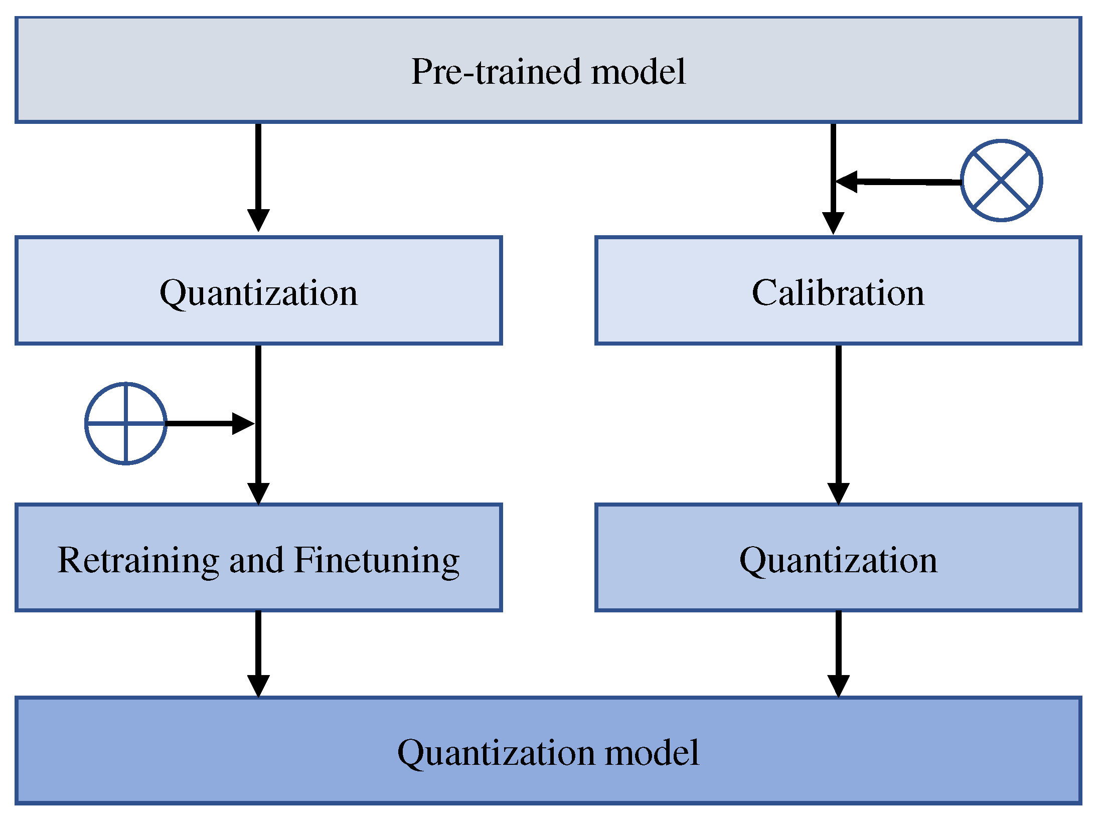
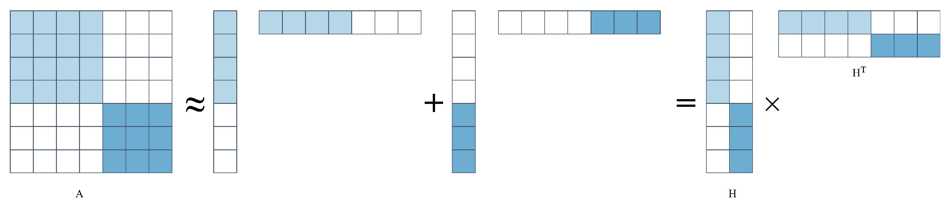
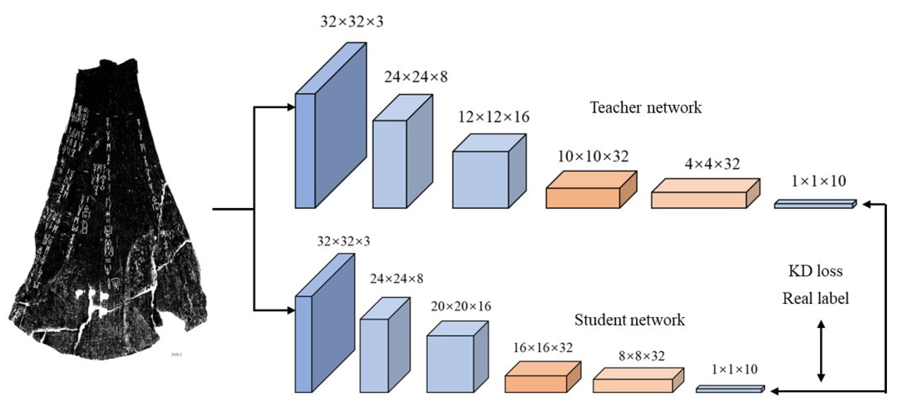
Table 1.
Classification accuracy and computation complexity of different DNN models on ImageNet. †
| Model | Layers | Parameter | FLOPs | Top-1 Error (%) |
|---|---|---|---|---|
| AlexNet [9] | 8 | 233(MB) | 4.4G | 43.45 |
| GoogLeNet [12] | 22 | 51(MB) | 8.9G | 34.20 |
| VGGNet-16 [11] | 16 | 528(MB) | 15.5G | 27.30 |
| VGGNet-19 [11] | 19 | 548(MB) | 19.7G | 25.50 |
| DenseNet-121 [14] | 121 | 31(MB) | 13.4G | 25.35 |
| ResNet-50 [13] | 50 | 98(MB) | 17.9G | 24.60 |
| ResNet-152 [13] | 152 | 230(MB) | 49.1G | 23.00 |
| ResNeXt-101 [15] | 101 | 319(MB) | 71.4G | 20.81 |
| SENet-154 [16] | 154 | 440(MB) | 93.8G | 18.68 |
† The FLOPs in the table are the number of floating operations the network makes in inferring a 512 × 512 image. The number of parameters is computed based on FP32.
Table 2.
Summary of different approaches for model compression.
| Core Idea | Operating Object | Architecture | Representative | Advantage | Disadvantage | |
|---|---|---|---|---|---|---|
| Model pruning | Designs parameter evaluation criteria to measure parameter importance. Removes unimportant parameters. | Con layer FC layer | Alter | Structured pruning, unstructured pruning. | Structured pruning narrows the network for hardware acceleration. Unstructured pruning compresses the network to any degree. | Structured pruning leads to accuracy reduction. Unstructured pruning leads to irregular architecture and is difficult to accelerate effectively. |
| Parameter quantization | Convers floating-point calculations to low-bitrate integer calculations. | Conv layer FC layer | Unaltered | Post-training quantization, quantization-aware training. | It reduces parameter storage space and memory, speeds up operation, and reduces equipment energy consumption. | It takes a long time to train and fine-tune and is inflexible. |
| Low-rank decomposition | Decomposes the original tensor into several low-rank tensors. | Conv layer. | Alter | Binary decomposition, multivariate decomposition. | It has good compression and acceleration effects on large convolution kernels and small and medium-sized networks. | Difficult to decompose simplified convolution kernels, layer-by-layer decomposition is not conducive to global parameter compression. |
| Knowledge distillation | Uses a large network with high complexity as a teacher network to guide low-complexity student networks. | Conv layer FC layer | Unaltered | Knowledge distillation for output layer, mutual information, correlation, and adversarial. | Large-scale models are compressed into small models and deployed to resource-constrained devices. | The network needs to be trained at least twice, and the training time is long. |
| Lightweight model design | Employs a compact and efficient network architecture and designs a network for deployment in mobile devices. | The entire network. | Alter | Convolution kernel level, layer level, network architecture level. | The network is simple, the training time is short, and the small network with a small storage amount, low calculation amount, and good performance can be obtained. | It is difficult to combine the special architecture with other compression and acceleration methods; poor generalization is not suitable as a pre-trained model to help other models. |
Table 3.
A simple comparison of the two methods is presented to measure the performance of each, based on the actual increases in speed and the compression ratio.
Table 3.
A simple comparison of the two methods is presented to measure the performance of each, based on the actual increases in speed and the compression ratio.
| Model | Top 5 Accuracy | Speed-Up | Compression Rate |
|---|---|---|---|
| AlexNet | 80.03% | 1.00 | 1.00 |
| BN Low-rank | 80.56% | 1.09 | 4.94 |
| CP Low-rank | 79.66% | 1.82 | 5.00 |
| VGG16 | 90.60% | 1.00 | 1.00 |
| BN Low-rank | 90.47% | 1.53 | 2.72 |
| CP Low-rank | 90.31% | 2.05 | 2.75 |
| GoogleNet | 92.21% | 1.00 | 1.00 |
| BN Low-rank | 91.88% | 1.08 | 2.79 |
| CP Low-rank | 91.79% | 1.20 | 2.84 |
Table 4.
Skills for lightweight models.
| Model | Methods |
|---|---|
| SqueezeNet [128] |
|
| SqueezeNext [131] |
|
| MobileNetV1 [129] |
|
| MobileNetV2 [132] |
|
| ShuffleNetV1 [130] |
|
| ShuffleNetV2 [133] |
|
Disclaimer/Publisher’s Note: The statements, opinions and data contained in all publications are solely those of the individual author(s) and contributor(s) and not of MDPI and/or the editor(s). MDPI and/or the editor(s) disclaim responsibility for any injury to people or property resulting from any ideas, methods, instructions or products referred to in the content. |
© 2023 by the authors. Licensee MDPI, Basel, Switzerland. This article is an open access article distributed under the terms and conditions of the Creative Commons Attribution (CC BY) license (https://creativecommons.org/licenses/by/4.0/).
Share and Cite
MDPI and ACS Style
Li, Z.; Li, H.; Meng, L. Model Compression for Deep Neural Networks: A Survey. Computers 2023, 12, 60. https://doi.org/10.3390/computers12030060
AMA Style
Li Z, Li H, Meng L. Model Compression for Deep Neural Networks: A Survey. Computers. 2023; 12(3):60. https://doi.org/10.3390/computers12030060
Chicago/Turabian StyleLi, Zhuo, Hengyi Li, and Lin Meng. 2023. "Model Compression for Deep Neural Networks: A Survey" Computers 12, no. 3: 60. https://doi.org/10.3390/computers12030060
Note that from the first issue of 2016, this journal uses article numbers instead of page numbers. See further details here.