

Convolutional Neural Networks: A Survey

1
Department of Information Technology, Faculty of Computer Science and Information Technology, Al-Baha University, Al-Baha 65528, Saudi Arabia
2
ReDCAD Laboratory, University of Sfax, Sfax 3038, Tunisia
Computers 2023, 12(8), 151; https://doi.org/10.3390/computers12080151
Submission received: 17 June 2023
/
Revised: 25 July 2023
/
Accepted: 25 July 2023
/
Published: 28 July 2023
(This article belongs to the Special Issue Artificial Intelligence Models, Tools and Applications with A Social and Semantic Impact)
Abstract
:Artificial intelligence (AI) has become a cornerstone of modern technology, revolutionizing industries from healthcare to finance. Convolutional neural networks (CNNs) are a subset of AI that have emerged as a powerful tool for various tasks including image recognition, speech recognition, natural language processing (NLP), and even in the field of genomics, where they have been utilized to classify DNA sequences. This paper provides a comprehensive overview of CNNs and their applications in image recognition tasks. It first introduces the fundamentals of CNNs, including the layers of CNNs, convolution operation (Conv_Op), Feat_Maps, activation functions (Activ_Func), and training methods. It then discusses several popular CNN architectures such as LeNet, AlexNet, VGG, ResNet, and InceptionNet, and compares their performance. It also examines when to use CNNs, their advantages and limitations, and provides recommendations for developers and data scientists, including preprocessing the data, choosing appropriate hyperparameters (Hyper_Param), and evaluating model performance. It further explores the existing platforms and libraries for CNNs such as TensorFlow, Keras, PyTorch, Caffe, and MXNet, and compares their features and functionalities. Moreover, it estimates the cost of using CNNs and discusses potential cost-saving strategies. Finally, it reviews recent developments in CNNs, including attention mechanisms, capsule networks, transfer learning, adversarial training, quantization and compression, and enhancing the reliability and efficiency of CNNs through formal methods. The paper is concluded by summarizing the key takeaways and discussing the future directions of CNN research and development.
1. Introduction
Artificial intelligence (AI) and classic programming represent two fundamentally different approaches to solving problems with machines [1,2]. Classical programming involves explicitly defining a set of rules and instructions for the machine to follow, which are based on the programmer’s understanding of the problem and the desired outcome. While classical programming can be effective for solving well-defined problems, it can quickly become unwieldy for complex tasks that involve a high degree of uncertainty or variability.
In contrast, AI involves training machines to learn from data and adapt their behavior based on experience, making it a more flexible and versatile approach to problem solving (Figure 1). AI systems can analyze large amounts of data, identify patterns and correlations, and use this information to make predictions or take actions without being explicitly programmed to do so. This makes AI particularly well-suited for tasks that involve complex decision making, such as natural language processing, image recognition, and autonomous driving.
Another key difference between AI and classical programming is the level of human intervention required [3]. In classical programming, the programmer must carefully design and write the program to achieve the desired outcome, often requiring significant time and effort. In contrast, AI systems can learn and improve on their own, reducing the need for human intervention and empowering machines to perform tasks that were previously thought to be beyond their capabilities [4,5].
AI has been a rapidly growing field in recent years, encompassing a range of techniques and approaches to enable machines to perform tasks that typically require human intelligence. With the increasing availability of data and advances in computing power, AI has become an essential tool for businesses and organizations to unlock insights, automate processes, and enhance decision-making capabilities [6,7].
The different phases of ML and AI include the following (Figure 2):
- Data collection: This refers to the process of gathering relevant data from various sources such as databases, APIs, or sensors, to use as input for machine learning or AI algorithms. The quality of the data collected will have a significant impact on the results produced by the algorithms.
- Data preprocessing: This involves cleaning, organizing, and transforming the raw data collected in the previous step into a format suitable for analysis. This includes tasks such as removing missing values, handling outliers, and scaling the data to ensure that it is normalized and consistent.
- Model selection and training: In this phase, a suitable machine learning or AI model is selected based on the specific problem being addressed. The model is then trained on the preprocessed data to learn patterns and make predictions. The training process involves adjusting the model parameters to minimize the error between predicted and actual values.
- Model evaluation: Once the model has been trained, it needs to be evaluated to assess its performance. This involves testing the model on a set of data that it has not seen before and comparing the predicted results to the actual values. Various metrics can be used to evaluate the model’s performance, such as accuracy, precision, recall, and F1 score.
- Deployment: After the model has been evaluated and validated, it can be deployed to perform the intended task. This involves integrating the model into a larger software system or application and providing a user interface for interaction with the model.
- Monitoring and maintenance: Once the model has been deployed, it is important to continuously monitor its performance and make necessary adjustments or updates to ensure that it remains accurate and effective. This includes tasks such as monitoring data input, tracking model behavior, and detecting potential errors or anomalies. Regular maintenance and updates are also required to keep the model up-to-date and relevant to changing conditions or requirements.
As illustrated in Figure 3, machine learning (ML) is a subset of AI that involves training machines on large datasets to learn patterns and make predictions [8]. Deep learning (DL) [9,10,11], which involves training neural networks with multiple layers, is a powerful subclass of ML that has shown remarkable success in various applications such as image and speech recognition [12,13].
Convolutional neural networks (CNNs) [14,15,16] are a popular type of ML model that have been widely utilized for various tasks, including image recognition [17,18,19,20], speech recognition [21,22,23,24,25], and NLP [26,27,28,29,30]. CNNs have been particularly successful in image recognition tasks, achieving state-of-the-art results on several benchmarks. Their success is due to their ability to capture spatial features and patterns in images by using a hierarchical architecture of layers that perform convolution operations and extract features at different levels of abstraction [31,32].
This paper provides a comprehensive overview of CNNs, covering their fundamentals, architectures, and recent developments. It also discusses the advantages and limitations of CNNs, provides recommendations for developers and data scientists, examines the existing platforms and libraries for CNNs, and estimates the cost of using CNNs. Our contributions include:
- A detailed discussion of the fundamentals of CNNs, including the layers of CNNs, the convolution operation, feature maps, activation functions, and training methods.
- A comparison of several popular CNN architectures, including LeNet, AlexNet, VGG, ResNet, and InceptionNet, and a discussion of their strengths and weaknesses.
- Recommendations for developers and data scientists on how to preprocess data, choose appropriate Hyper_Param, use regularization techniques, and evaluate model performance.
- A discussion of existing platforms and libraries for CNNs, including TensorFlow, Keras, PyTorch, Caffe, and MXNet, and a comparison of their features and functionalities.
- An estimation of the cost of using CNNs, including factors that impact cost such as hardware, dataset size, and model complexity, as well as potential cost-saving strategies.
- An examination of when to use CNNs, including tasks suited for CNNs, their computational requirements, and their advantages and limitations.
- A review of the security aspects of CNNs, including potential vulnerabilities and strategies for improving the security of CNNs.
- A discussion of the future directions of CNN research and development.
The paper is organized as follows: Section 2 provides an overview of the fundamentals of convolutional neural networks (CNNs), and Section 3 compares several popular CNN architectures. Section 4 explains the situations in which it is appropriate to use CNNs, and Section 5 discusses the advantages and limitations of CNNs. Section 6 describes some existing platforms and libraries to create CNN models, while Section 7 compares CNN models with other models. Next, Section 8 provides recommendations for developers and data scientists, and Section 9 estimates the cost of using CNNs. Section 10 reviews recent developments in CNNs, and Section 11 discusses the use of formal methods for enhancing the reliability and efficiency of CNNs. Finally, the paper concludes in Section 12.
2. Fundamentals of CNNs
CNNs are a powerful type of neural network that are widely used in image recognition tasks. They consist of a series of convolutional and pooling layers that extract relevant features from the input image, followed by one or more fully connected layers that use these features to make a prediction. To use a CNN for image recognition, it must first be trained on a large dataset of labeled images containing the objects of interest. During training, the CNN learns to associate the extracted features with the correct labels through a process of back propagation and optimization [35,36,37,38]. Once the CNN has been trained, it can be used to make predictions on new, unseen images by passing the image through the network and selecting the label with the highest predicted probability.
Figure 4 shows a simplified illustration of a CNN used for image classification [39,40,41]. The input of the network is an image of a car, which is fed into the input layer. The input layer passes the image to the first hidden layer, which applies a set of filters to the image. Each filter extracts specific features from the image, such as edges or textures. The output of the first hidden layer is then passed to the next hidden layer, where more filters are applied to extract higher-level features. This process is repeated through several hidden layers until the final hidden layer, which produces a set of features that are passed to the output layer. The output layer produces a probability distribution over the three classes: car, bus, and plane. The network then makes a decision based on the class with the highest probability. The weights of the filters in each layer are learned through a process called back propagation, which adjusts the weights to minimize the error between the predicted output and the actual output.
2.1. Layers of CNNs
A CNN typically consists of multiple layers, each with a specific function in the network:
- Convolutional layer: The convolutional layer is the core building block of a CNN [42,43]. It performs a convolution operation on the input image with a set of learnable filters. The filters are small matrices that slide over the input image, computing a dot product between the filter and a small region of the input at each step. The output of the convolutional layer is a set of feature maps that represent different features in the input image.
- Pooling layer: The pooling layer is used to reduce the spatial dimensions of the feature maps produced by the convolutional layer [44,45]. It operates on each feature map independently and downsamples it by taking the maximum or average value of non-overlapping regions. Pooling helps to reduce the computational complexity of the network and also makes the network more robust to small translations in the input image.
In addition to these layers, there are also specialized layers that are used in certain types of CNNs. For example, in a recurrent CNN (RCNN), a recurrent layer is added to the network to capture temporal dependencies in the input sequence [57,58]. In a long short-term memory (LSTM) CNN, an LSTM layer is used to learn long-term dependencies in the input sequence [59,60,61].
Table 1 presents a summary of the layers commonly used in CNNs and their respective functions in the network. Overall, the different types of layers in a CNN work together to learn and extract features from the input image, and ultimately produce an accurate prediction or classification. By understanding the role of each layer, researchers and practitioners can design more effective CNN architectures for a wide range of computer vision tasks [62,63,64].
2.2. Convolution Operation
The convolution operation (Conv_Op) is a mathematical operation that is commonly used in signal processing, image processing, and computer vision [65,66,67]. It is used to combine two signals or functions to produce a third signal that represents the influence of one signal on the other, weighted by the shape of the other signal. In computer vision, convolution is used to extract features from images using CNNs.
The mathematical definition of the convolution operation is:
Here, f and g are two functions that can be discrete or continuous, and n is the position or time index of the output signal. The convolution operation is denoted by the symbol ∗. When the input signals are discrete, the above equation can be written as:
where is the sampling interval. When the input signals are continuous, the convolution operation can be defined as:
where t is the time index of the output signal.
In computer vision, the convolution operation is used to extract features from an image using CNNs. The Conv_Op is a fundamental operation in CNNs that involves sliding a filter or kernel over an input image and computing the dot product at each position to produce an output feature map.
The Conv_Op is applied to each channel of the input image separately, and the resulting feature maps are combined to form the output. The size of the filter is a crucial parameter that determines the size of the receptive field, which is the region of the input that affects the output at a particular position. The stride determines the distance between adjacent filter positions. The amount of zero padding around the input image can also be adjusted to control the size and resolution of the output feature map.
The Conv_Op can be performed using various methods, including the direct method, the Fourier method, and the fast Fourier transform (FFT) method [68,69,70,71,72,73]. The direct method is the most straightforward, but it can be computationally expensive, especially for large input volumes and filters. The Fourier method and the FFT method can significantly speed up the convolution operation by exploiting the convolution theorem, which states that convolution in the spatial domain is equivalent to multiplication in the frequency domain.
In summary, convolution is a mathematical operation that is used to combine two signals or functions to produce a third signal that represents the influence of one signal on the other, weighted by the shape of the other signal. In computer vision, convolution is used to extract features from images using CNNs. The Conv_Op involves sliding a filter over an input image and computing the dot product at each position to produce an output feature map. The size of the filter, the stride, and the amount of zero padding are adjustable parameters that can be used to control the size and resolution of the output. The convolution operation can be performed using various methods, and the choice of activation function is also an important consideration.
2.3. Feature Maps
In CNNs, a feature map (Feat_Map) is a crucial component that represents the output of a convolutional layer [74,75,76,77,78,79]. The Feat_Map is a two-dimensional array that reflects the degree to which the local regions of the input image match the filters that were applied to them. Each element of the Feat_Map corresponds to the activation of a neuron in the layer and captures some specific aspect of the input image.
The Feat_Map is computed by convolving a set of filters with the input image. Each filter generates a single-channel Feat_Map that highlights a specific feature or pattern in the input image. The Feat_Maps produced by different filters in the same layer can be stacked together to create a multi-channel Feat_Map that captures different aspects of the input image.
Mathematically, the computation of a Feat_Map can be represented as:
where is the value of the k-th Feat_Map at position in the output tensor, is the weight of the k-th filter at position , is the value of the n-th input Feat_Map at position , and is the bias term for the k-th Feat_Map.
In this equation, F represents the height and width of the filter, represents the number of channels in the input tensor, and is a scalar bias term that is added to each element of the k-th Feat_Map. The weights are learned during the training process using back propagation and gradient descent, and they determine how each filter responds to the local regions of the input image.
The computation of a Feat_Map involves sliding the filter over the input image and computing the dot product between the filter and the corresponding local region of the input image at each position. The resulting values are then summed and passed through an activation function to obtain the final values of the Feat_Map. This process is repeated for each filter in the layer, resulting in a set of Feat_Maps that collectively capture different aspects of the input image.
Overall, the Feat_Map is a powerful tool in CNNs that allows them to extract and capture important features from the input image, enabling them to perform a wide range of visual recognition tasks.
2.4. Activation Functions
Activation functions (Activ_Funcs) are an essential component in CNNs that introduce non-linearity into the model [80,81,82,83,84,85]. This non-linearity is crucial because many real-world phenomena exhibit complex, non-linear behavior, and a model that only uses linear operations will not be able to capture these phenomena accurately. Thus, Activ_Funcs help to make CNNs more expressive and able to model a wider range of functions.
Commonly used Activ_Funcs in CNNs include the rectified linear unit (ReLU), the sigmoid function, and the hyperbolic tangent (tanh) function (Figure 5). ReLU is the most widely used Activ_Func in modern CNNs because of its simplicity and effectiveness in reducing the vanishing gradient problem during training.
Mathematically, the ReLU Activ_Func is defined as:
where x is the input to the neuron. This function returns the maximum of 0 and x, effectively “turning off” any negative values and leaving positive values unchanged. This simple non-linear function allows for better learning of complex features in CNNs and helps to prevent the saturation of neurons during training.
The sigmoid function, on the other hand, is defined as:
where x is the input to the neuron. The sigmoid function has a characteristic S-shape and maps any real number to a value between 0 and 1, making it a good choice for binary classification problems. However, it suffers from the vanishing gradient problem when used in deep neural networks due to its saturating nature, which can slow down the training process.
The hyperbolic tangent (tanh) function is similar to the sigmoid function but maps any real number to a value between −1 and 1. It is also a non-linear function that is useful for introducing non-linearity into the model. However, like the sigmoid function, it can suffer from the vanishing gradient problem in deep neural networks.
In addition to these commonly used Activ_Funcs, there are also other functions such as the softmax function, which is used in the output layer of CNNs for multi-class classification problems. The softmax function maps the output of the last layer to a probability distribution over the classes, making it suitable for probability-based classification tasks.
Overall, the choice of Activ_Funcs in CNNs can have a significant impact on the performance and convergence of the model. Different functions have different strengths and weaknesses, and choosing the right function for the task at hand is an important part of designing a successful CNN.
2.5. Padding, Stride, and Filters
Padding, stride, and filters are important parameters in CNNs that determine the size and resolution of the output feature maps (Feat_Maps) [86,87,88,89,90,91,92,93]. These parameters play a crucial role in controlling the amount of information that is retained in the Feat_Maps and can greatly impact the performance of the network.
Padding involves adding extra rows and columns of zeros around the input image before applying the filters. This can help to preserve the spatial dimensions of the image as it passes through the convolutional layers. Padding is typically used to ensure that the output Feat_Maps have the same spatial dimensions as the input image or to control the size of the output Feat_Maps.
Stride is another important parameter in CNNs that determines the distance between adjacent filter positions as the filter is slid over the input image. By adjusting the stride, it is possible to control the resolution of the output Feat_Maps. A larger stride results in a lower resolution output Feat_Map, while a smaller stride leads to a higher resolution output Feat_Map.
Filters are the small matrices that are applied to the input image to produce the Feat_Map. The filters are learned during the training process, and their values are updated using back propagation. The size of the filter is an important parameter that determines the size and complexity of the features that the filter can capture. Larger filters can capture more complex features but require more computation and are more prone to overfitting.
The size of the output Feat_Map depends on the size of the input image, the size of the filter, the stride, and the amount of padding. The output Feat_Map size can be calculated using the following formula:
where W is the width (or height) of the input image, F is the width (or height) of the filter, P is the amount of padding, and S is the stride. This formula gives the number of positions where the filter can be applied to the input image to produce the output Feat_Map.
Adjusting the padding, stride, and filter size is an important part of designing a CNN architecture that can effectively capture the features of the input image and produce high-quality Feat_Maps. These parameters provide a degree of flexibility in the design of convolutional layers, allowing the network to be tailored to the specific task at hand. For example, a network designed for image classification may use larger filters and smaller strides to capture more complex features, while a network designed for object detection may use smaller filters and larger strides to reduce the computation required and speed up the detection process.
Overall, understanding the role of padding, stride, and filters in CNNs is critical for designing effective neural network architectures that can accurately capture and classify complex visual patterns in images and other signals.
2.6. Training CNNs
Training a CNN involves adjusting the weights and biases of the model so that it produces accurate predictions on the training data [94,95,96,97,98,99]. This is achieved using an optimization algorithm that minimizes a loss function (Loss_Func), which measures the difference between the predicted output of the model and the true output. The most commonly utilized optimization algorithm for training CNNs is stochastic gradient descent (SGD), which updates the weights and biases of the model in small steps based on the gradient of the Loss_Func with respect to these parameters. The process of updating the weights and biases using the gradient is called back propagation, and it involves propagating the error from the output layer (Out_Lay) back through the network to update the weights and biases of each layer. This is achieved using the chain rule of calculus to compute the derivative of the Loss_Func with respect to each parameter in the network. The learning rate is a Hyper_Param that controls the size of the updates made to the weights and biases at each iteration of the optimization algorithm. It is important to choose a suitable learning rate, as a value that is too small may cause the optimization algorithm to converge slowly, while a value that is too large may cause the algorithm to overshoot the optimal weights and biases and fail to converge. Other Hyper_Params that can be tuned to improve the performance of the model include the number of layers in the network, the size of the filters, the number of filters in each layer, the type of Activ_Func utilized, and the amount of padding and stride utilized in the convolutional layers and Pool_Lays.
2.7. Back Propagation
Back propagation is an algorithm utilized to efficiently compute the gradients of the Loss_Func with respect to the weights and biases of a neural network [100,101,102,103]. It works by propagating the error from the Out_Lay back through the network and computing the derivative of the Loss_Func with respect to each parameter in the network using the chain rule of calculus. The back propagation algorithm is utilized in conjunction with an optimization algorithm to update the weights and biases of the network during training. An illustration of this notion is shown in Figure 6.
Mathematically, the back propagation algorithm can be represented as:
- Compute the output of the network for a given input.
- Compute the error between the predicted output and the true output.
- Compute the gradient of the Loss_Func with respect to the output of the network.
- Use the chain rule to compute the gradient of the Loss_Func with respect to the weights and biases of each layer in the network:where L is the Loss_Func, is the weight connecting neuron i in layer to neuron j in layer l, is the bias of neuron i in layer l, and is the weighted sum of the inputs to neuron i in layer l.
- Update the weights and biases of the network using an optimization algorithm.
- Repeat steps 1–5 for each training example.
- Repeat steps 1–6 for a fixed number of epochs or until convergence.
2.8. Optimization Algorithms
Optimization algorithms are utilized to update the weights and biases of a neural network during training to minimize the Loss_Func [104,105]. The most commonly utilized optimization algorithm for training neural networks is stochastic gradient descent (SGD), which updates the weights and biases of the network in small steps based on the gradient of the Loss_Func with respect to these parameters.
Other optimization algorithms that have been developed include the following:
- Momentum: This algorithm adds a momentum term to the gradient update, which helps to smooth out the updates and accelerate convergence. The update rule for momentum can be written as:where is the momentum at time t, is the momentum coefficient, is the gradient of the Loss_Func with respect to the weights at time , is the learning rate, and is the updated weights.
- AdaGrad: This algorithm adapts the learning rate for each weight based on the magnitude of the gradients seen so far, which allows for faster convergence on flat directions and slower convergence on steep directions. The update rule for AdaGrad can be written as:where is the diagonal matrix of sums of squares of past gradients up to time t, is a small constant to avoid division by zero, and all other variables are as previously defined.
- RMSProp: This algorithm uses a moving average of the squared gradients to adapt the learning rate for each weight, which helps to prevent the learning rate from becoming too large. The update rule for RMSProp can be written as:where is the moving average of the squared gradients up to time t, is the decay rate, and all other variables are as previously defined.
- Adam: This algorithm combines ideas from momentum and AdaGrad to create an adaptive learning rate algorithm that works well in practice for a wide range of neural networks. The update rule for Adam can be written as:where and are the first and second moment estimates of the gradients, and are the decay rates for the first and second moments, and are bias-corrected estimates of the first and second moments, is a small constant to avoid division by zero, and all other variables are as previously defined.
Table 2 summarizes several optimization algorithms that are commonly used to update the weights and biases of neural networks during training to minimize the Loss_Func, including SGD, momentum, AdaGrad, RMSProp, and Adam, each with their own unique characteristics that can have a significant impact on the performance of the network.
2.9. Regularization Techniques
Regularization techniques are utilized to prevent overfitting in neural networks, which occurs when the model performs well on the training data but poorly on new unseen data [106,107,108,109,110]. Regularization techniques work by adding a penalty term to the Loss_Func that encourages the model to have simpler weights or to reduce the magnitude of the weights.
Some commonly utilized regularization techniques include:
- L1 regularization: This technique adds a penalty to the Loss_Func proportional to the absolute value of the weights, which encourages the model to have sparse weights and can lead to feature selection [111,112,113,114]. The regularized Loss_Func for L1 regularization can be written as:where is the original Loss_Func, is the ith weight in the network, n is the total number of weights, and is the regularization strength.
- L2 regularization: This technique adds a penalty to the Loss_Func proportional to the square of the weights, which encourages the model to have small weights and can help to prevent overfitting [115,116,117,118]. The regularized Loss_Func for L2 regularization can be written as:where all variables are as previously defined.
- Dropout: This technique randomly drops out some of the neurons in the network during training, which helps to prevent the model from relying too heavily on any one feature and can improve generalization performance [119,120,121]. The dropout regularization can be implemented by randomly setting the output of each neuron to zero with a certain probability p during training. The dropout regularization can be written as:where y is the output of a layer, is the regularized output, r is a binary mask that is randomly generated for each training example, and ⊙ denotes element-wise multiplication. During testing, the dropout is turned off and the output is scaled by to compensate for the effect of dropout.
- Early stopping: This technique stops the training process early based on a validation set performance metric, which helps to prevent the model from overfitting to the training data [122,123,124,125]. The idea is to monitor the validation loss or accuracy during training and stop the training process when the validation
Table 3 summarizes several commonly utilized regularization techniques for preventing overfitting in neural networks, including L1 and L2 regularization, dropout, and early stopping, each with their own unique approach to encouraging simpler weights or preventing over-reliance on any one feature, ultimately improving the generalization performance of the model.
2.10. Evaluation Metrics
One of the most common challenges faced by training algorithms is the need to prevent overfitting, which is addressed in this study through the use of regularization. To assess the learning performance of the CNN model, a confusion matrix is employed as a conventional evaluation technique. In the field of image categorization, the confusion matrix is used to evaluate the predicted results against the actual values and measure the model’s performance. Through the confusion matrix, we can not only identify accurate and inaccurate predictions but also gain insights into the specific types of errors made. To calculate the confusion matrix, a set of test data and validation data containing the obtained results’ values are required. This traditional method can be used to identify six types of welding flaws, and the evaluation measure is depicted in Figure 7.
The results are divided into four categories:
- True positive (): The “true positive” category in the confusion matrix represents the number of instances in which the model accurately predicts the positive class or event out of all the true positive instances in the dataset.
- True negative (): In the confusion matrix, “true negative” refers to the number of instances in which the model correctly predicts the negative class out of all the true negative instances in the dataset.
- False positive (): The “false positive” represents the model’s error when it incorrectly predicts the presence of a specific condition or event that is not actually present. This type of error is also called a type I error and can lead to incorrect decisions if not properly managed.
- False negative (): A “false negative” in the confusion matrix is when the model incorrectly predicts the absence of an event among all actual positive instances in the data. It measures the model’s tendency to miss positive cases or make type II errors.
3. CNN Architectures
Over the years, several different CNN architectures have been developed, each with its own unique features and performance characteristics.
3.1. LeNet
LeNet is one of the earliest CNN architectures, developed by Yann L.C. et al. in 1998 for recognizing handwritten digits. The LeNet architecture consists of two Conv_Lays, followed by two fully connected layers [126,127,128,129]. The Conv_Lays use small filters and Pool_Lays to extract features from the input image, and the fully connected layers use a softmax activation to output a probability distribution over the possible classes.
Mathematically, the LeNet architecture can be represented as:
- Conv_Lay with 6 filters of size 5 × 5, followed by a 2 × 2 max Pool_Lay.
- Conv_Lay with 16 filters of size 5 × 5, followed by a 2 × 2 max Pool_Lay.
- Fully connected layer with 120 units and a sigmoid Activ_Func.
- Fully connected layer with 84 units and a sigmoid Activ_Func.
- Out_Lay with 10 units and a softmax Activ_Func.
3.2. AlexNet
AlexNet is a CNN architecture developed by Alex Krizhevsky et al. in 2012, which achieved state-of-the-art performance on the ImageNet dataset [130,131,132]. The AlexNet architecture consists of five Conv_Lays, followed by three fully connected layers. The Conv_Lays use larger filters than LeNet and also include local response normalization and overlapping Pool_Lays. The fully connected layers use ReLU activation to introduce non-linearity into the network.
Mathematically, the AlexNet architecture can be represented as:
- Conv_Lay with 96 filters of size 11 × 11, followed by a 2 × 2 max Pool_Lay.
- Conv_Lay with 256 filters of size 5 × 5, followed by a 2 × 2 max Pool_Lay.
- Conv_Lay with 384 filters of size 3 × 3.
- Conv_Lay with 384 filters of size 3 × 3.
- Conv_Lay with 256 filters of size 3 × 3, followed by a 2 × 2 max Pool_Lay.
- Fully connected layer with 4096 units and a ReLU Activ_Func.
- Fully connected layer with 4096 units and a ReLU Activ_Func.
- Out_Lay with 1000 units and a softmax Activ_Func.
3.3. VGG
VGG is a CNN architecture developed by Karen Simonyan and Andrew Zisserman in 2014, which achieved state-of-the-art performance on the ImageNet dataset [133,134,135,136,137]. The VGG architecture consists of multiple layers of small 3 × 3 convolutional filters, followed by max Pool_Lays. The fully connected layers use ReLU activation and dropout regularization to prevent overfitting.
Mathematically, the VGG architecture can be represented as:
- Conv_Lay with 64 filters of size 3 × 3, followed by a 2 × 2 max Pool_Lay.
- Conv_Lay with 128 filters of size 3 × 3, followed by a 2 × 2 max Pool_Lay.
- Conv_Lay with 256 filters of size 3 × 3, followed by a 2 × 2 max Pool_Lay.
- Conv_Lay with 512 filters of size 3 × 3, followed by a 2 × 2 max Pool_Lay.
- Conv_Lay with 512 filters of size 3 × 3, followed by a 2 × 2 max Pool_Lay.
- Fully connected layer with 4096 units and a ReLU Activ_Func, followed by dropout regularization.
- Fully connected layer with 4096 units and a ReLU Activ_Func, followed by dropout regularization.
- Out_Lay with 1000 units and a softmax Activ_Func.
3.4. ResNet
ResNet is a CNN architecture developed by Kaiming He et al. in 2015, which introduced the concept of residual connections to address the problem of vanishing gradients in deep networks [138,139,140,141,142,143]. The ResNet architecture consists of multiple residual blocks, each of which includes multiple Conv_Lays and shortcut connections that bypass the Conv_Lays and add the original input to the output of the block. The fully connected layers use a softmax activation to output a probability distribution over the possible classes.
Mathematically, the ResNet architecture can be represented as:
- Conv_Lay with 64 filters of size 7 × 7, followed by a 3 × 3 max Pool_Lay.
- Multiple residual blocks, each of which consists of:
- Conv_Lay with 64 filters of size 3 × 3.
- Conv_Lay with 64 filters of size 3 × 3.
- Shortcut connection that adds the original input to the output of the block.
- Multiple residual blocks, each of which consists of:
- Conv_Lay with 128 filters of size 3 × 3, followed by a 2 × 2 max Pool_Lay.
- Conv_Lay with 128 filters of size 3 × 3.
- Conv_Lay with 128 filters of size 3 × 3.
- Shortcut connection that adds the original input to the output of the block.
- Multiple residual blocks, each of which consists of:
- Conv_Lay with 256 filters of size 3 × 3, followed by a 2 × 2 max Pool_Lay.
- Conv_Lay with 256 filters of size 3 × 3.
- Conv_Lay with 256 filters of size 3 × 3.
- Shortcut connection that adds the original input to the output of the block.
- Multiple residual blocks, each of which consists of:
- Conv_Lay with 512 filters of size 3 × 3, followed by a 2 × 2 max Pool_Lay.
- Conv_Lay with 512 filters of size 3 × 3.
- Conv_Lay with 512 filters of size 3 × 3.
- Shortcut connection that adds the original input to the output of the block.
- Fully connected layer with 1000 units and a softmax Activ_Func.
3.5. InceptionNet
InceptionNet, also known as GoogLeNet, is a CNN architecture developed by Christian Szegedy et al. in 2014, which introduced the concept of inception modules to allow for efficient use of computational resources [144,145,146,147,148]. Inception modules consist of multiple convolutional filters of different sizes and Pool_Lays, which are concatenated together to form the output of the module. The InceptionNet architecture also includes auxiliary classifiers to help with training and to regularize the network.
Mathematically, the InceptionNet architecture can be represented as:
- Conv_Lay with 64 filters of size 7 × 7, followed by a 2 × 2 max Pool_Lay.
- Conv_Lay with 64 filters of size 1 × 1, followed by a Conv_Lay with 192 filters of size 3 × 3, and a 2 × 2 max Pool_Lay.
- Multiple inception modules, each of which consists of:
- Conv_Lay with 64 filters of size 1 × 1.
- Conv_Lay with 96 filters of size 3 × 3.
- Conv_Lay with 128 filters of size 5 × 5.
- Max Pool_Lay with a 3 × 3 filter and stride 1.
- Concatenation of the outputs of the previous layers.
- Multiple inception modules, each of which consists of:
- Conv_Lay with 192 filters of size 1 × 1.
- Conv_Lay with 96 filters of size 3 × 3.
- Conv_Lay with 208 filters of size 5 × 5.
- Max Pool_Lay with a 3 × 3 filter and stride 1.
- Concatenation of the outputs of the previous layers.
- Multiple inception modules, each of which consists of:
- Conv_Lay with 160 filters of size 1 × 1.
- Conv_Lay with 112 filters of size 3 × 3.
- Conv_Lay with 224 filters of size 5 × 5.
- Max Pool_Lay with a 3 × 3 filter and stride 1.
- Concatenation of the outputs of the previous layers.
3.6. Comparison of CNN Architectures
The goal of this section is to provide a comparison of the key details and performance of several popular CNN architectures, including LeNet, AlexNet, VGG, ResNet, and InceptionNet. The details of each architecture, including the number of layers, filters, and top-1 and top-5 error rates, are summarized in Table 4.
Note that the number of layers and filters is approximate, as it varies depending on the specific implementation of each architecture. The top-1 and top-5 error rates are the percentage of images in the ImageNet dataset that are misclassified by the model, with the top-1 error rate indicating the percentage of images for which the correct class is not in the top predicted class, and the top-5 error rate indicating the percentage of images for which the correct class is not in the top-5 predicted classes.
In terms of performance, ResNet and InceptionNet have achieved the lowest error rates on the ImageNet dataset, with ResNet achieving a top-5 error rate of just 1.6%. VGG also achieved impressive performance, with a top-5 error rate of 8.7%. AlexNet achieved a top-5 error rate of 17.0%, which was a significant improvement over previous state-of-the-art models at the time. LeNet was one of the earliest CNN architectures and was designed for recognizing handwritten digits, so its performance is not directly comparable to the other architectures.
One notable trend in these architectures is the increasing depth of the models over time. LeNet had just 5 layers, while AlexNet had 8 and VGG had 19. ResNet and InceptionNet took this trend to the extreme, with ResNet having 152 layers and InceptionNet having 22 layers. However, these architectures also introduced new techniques to help with training deeper models, such as residual connections and inception modules.
Another trend is the use of smaller filters, which allows for more layers to be added without significantly increasing the number of parameters in the model. LeNet utilized 5 × 5 filters, while AlexNet utilized a mix of 11 × 11 and 5 × 5 filters. VGG utilized only 3 × 3 filters, which allowed for a very deep architecture with relatively few parameters. ResNet and InceptionNet also utilized a mix of small filters, with InceptionNet using a variety of filter sizes in its inception modules.
Overall, each of these architectures has made important contributions to the field of computer vision and deep learning (DL). LeNet was one of the first successful CNN architectures, while AlexNet demonstrated the potential of DL for image classification tasks. VGG showed that very deep architectures could achieve state-of-the-art performance, while ResNet and InceptionNet introduced new techniques for training even deeper models.
4. When to Use CNN?
4.1. Some Examples
Table 5 summarizes selected research papers and their key findings related to the use of CNNs, including automated welding fault detection, lip reading, olive leaf disease detection, mask recognition for COVID-19, visual spam classification, and driver sleepiness detection. The table highlights the proposed methods, the accuracy rates achieved, and the potential applications of the developed models. More details about each example are provided next.
The proposed method in [149] uses a convolutional neural network (CNN) and data augmentation to identify multi-class welding errors in X-ray pictures (see Figure 8 and Figure 9). Detecting weld faults with X-rays is expensive and time consuming, requiring experienced specialists who may make mistakes owing to weariness and distraction. Data augmentation techniques such as random rotation, shearing, zooming, brightness adjustment, and horizontal flips are used to train a generalized CNN network to identify welding flaws in a multi-class dataset. The suggested approach is tested using 4479 industrial X-ray images of cavity, cracks, inclusion slag, absence of fusion, shape defects, and normal flaws. The proposed method for automated welding flaw detection and categorization had a 92% accuracy rate. Thus, this work proposes an automated method for detecting multi-class welding faults in X-ray pictures using data augmentation and a CNN, which could reduce manual inspection expenses and errors.
The work reported in [150] developed a Kannada language dataset and machine-learning-based VSR technique. VSR is a lip-reading method that can help hearing-impaired, laryngeal, and loud people. The authors created a dataset of five random Kannada sentences with an average video time of 1 to 1.2 s. Using a VGG16 CNN and ReLU activation function, they extracted and classified features with 91.90% accuracy. The suggested system outperformed HCNN, ResNet-LSTM, Bi-LSTM, and GLCM-ANN. Thus, this work developed a novel dataset and machine-learning-based VSR technique for Kannada, which may aid hearing-impaired or loud people.
The work discussed in [151] developed a novel deep ensemble learning technique that uses CNN and vision transformer models to detect and classify olive leaf illnesses. Disease detection algorithms based on deep learning are becoming increasingly essential in agriculture, but the diversity of plant species and regional features of many species make them difficult to build. Due to the range of pathogens that can infect olive groves, olive leaf diseases are difficult to diagnose. The authors built binary and multi-classification methods using deep convolutional models. The proposed deep ensemble learning technique uses CNN and vision transformer models to achieve 96% multi-class classification accuracy and 97% binary classification accuracy, beating other models. This study suggests that the proposed approach could detect and classify olive leaf illnesses, which could assist olive growers by enabling timely disease identification and treatment. Thus, the work developed a novel deep ensemble learning technique for olive leaf disease detection and classification, which could increase olive grove profitability and sustainability.
The work discussed in [105] developed a strong mask detection model utilizing computer vision to tackle COVID-19. The authors remark that the COVID-19 epidemic has motivated the artificial intelligence community to research new ways to fight the disease, and computer vision, a sub-discipline of AI, has been effective in many sectors. The authors have since contributed a few articles using computer vision for COVID-19 tasks. The suggested mask detection model can identify persons wearing prescribed masks, those not wearing masks, and those not wearing masks properly. Experiments prove the model’s power and robustness. Thus, this work developed a computer vision-based mask recognition algorithm to help battle COVID-19 by detecting those who are not wearing masks or wearing them improperly.
The work discussed in [152] explores visual spam classification using deep convolutional neural networks (DCNNs) and transfer-learning-based pre-trained CNN models. Image spam, which uses images to bypass text-based spam filters, was classified using two DCNN models and several pre-trained ImageNet architectures on three datasets. Cost-sensitive learning was also tested for data imbalance. In the best situation, several of the presented models approach 99% accuracy with zero false positives, improving picture spam classification. This study proposes employing DCNNs and transfer-learning-based pre-trained CNN models to improve visual spam categorization.
The work discussed in [153] developed a neural-network-based approach for detecting driver micro-naps and sleepiness. In this work, the authors use facial landmarks detected by a camera as input to a convolutional neural network to categorize tiredness instead of a multi-layer perceptron. The suggested CNN-based model obtains high accuracy rates, with more than 88% for the category without glasses, more than 85% for the category night without glasses, and an overall average accuracy of more than 83% in all categories. The proposed model has a maximum size of 75 KB and is smaller, simpler, and more storage-efficient than the benchmark model. This lightweight and accurate CNN-based model might be used to construct a real-time driver sleepiness detection system for embedded systems and Android devices, according to the authors. Thus, this work proposes a lightweight classification model for driver sleepiness detection that is accurate and easy to use.
4.2. Tasks Suited for CNNs
CNNs are particularly well-suited for tasks that involve analyzing visual data, such as image classification, object detection, and segmentation. This is because CNNs are able to learn hierarchical representations of visual data, where higher-level features are built upon lower-level features, allowing the model to understand complex patterns in the data and make accurate predictions.
CNNs are also well-suited for tasks that involve analyzing sequential data, such as speech recognition and NLP, where the data has a spatial or temporal structure that can be exploited by the Conv_Lays. For example, in speech recognition, the input waveform can be viewed as a sequence of frames, and the Conv_Lays can be utilized to extract features from these frames that capture the phonetic content of the speech. In NLP, the Conv_Lays can be utilized to extract features from the input text that capture the meaning of the words and their relationships to each other.
4.3. Best Utilized with Large Amounts of Training Data
CNNs require a large amount of labeled training data to perform well. This is because the models have millions of parameters that need to be learned from the data, and they require a significant amount of variation in the data to avoid overfitting. In general, the more data that is available for training, the better the performance of the model will be. However, collecting large amounts of labeled training data can be time consuming and expensive, especially for tasks that involve fine-grained classification or segmentation. In such cases, transfer learning can be a useful technique, where a pre-trained model is utilized as a starting point and fine-tuned on a smaller dataset. This can significantly reduce the amount of labeled data required for training and improve the performance of the model.
It is also worth noting that CNNs can be sensitive to the quality of the training data. If the data is noisy or contains biases, the model may learn to recognize these artifacts rather than the underlying patterns in the data. Therefore, it is important to carefully curate and preprocess the training data to ensure that it is representative of the task at hand.
4.4. Computational Requirements
Training CNNs can be computationally expensive, especially for large models with many layers. This is because CNNs typically require a lot of memory and processing power to train. However, recent advances in hardware and software have made it possible to train large CNNs on a single GPU or even multiple GPUs in parallel.
In addition to the computational requirements for training, there are also computational requirements for inference, where the model is utilized to make predictions on new data. The computational requirements for inference depend on the size of the model and the complexity of the task, but they are generally less than the requirements for training. In some cases, it may be necessary to optimize the model architecture or use specialized hardware, such as tensor processing units (TPUs), to achieve real-time performance.
To reduce the computational requirements of training and inference, various techniques have been developed, including model pruning, quantization, and compression. These techniques aim to reduce the size of the model and the number of operations required for inference, without significantly degrading the performance of the model. Additionally, pre-trained models are available for many tasks, which can significantly reduce the computational requirements for training new models. These pre-trained models can be fine-tuned on a smaller dataset, which can lead to improved performance and reduced training time.
Overall, while CNNs can be computationally expensive, they are a powerful tool for analyzing visual and sequential data. They are best suited for tasks that require the analysis of complex patterns in the data and are most effective when trained on large amounts of labeled data. With recent advances in hardware and software, CNNs are becoming increasingly accessible to researchers and practitioners, and are likely to continue to play a significant role in the field of ML and computer vision.
5. Advantages and Limitations of CNNs
5.1. Advantages
CNNs have several advantages that make them a powerful tool for analyzing visual and sequential data. One of the main advantages of CNNs is their ability to learn hierarchical representations of the input data, where higher-level features are built upon lower-level features. This allows the model to understand complex patterns in the data and make accurate predictions.
Another advantage of CNNs is their ability to handle inputs of varying sizes and aspect ratios. This is because the Conv_Lays are able to learn features that are translation-invariant, meaning that they can recognize the same pattern regardless of its location in the input. Additionally, max-pooling layers can be utilized to downsample the input, allowing the model to handle inputs of varying sizes and aspect ratios.
CNNs also have the ability to generalize well to new data, meaning that they are able to make accurate predictions on data that they have not seen before. This is because the models learn features that are relevant to the task, rather than memorizing specific examples from the training data. Additionally, transfer learning can be utilized to transfer knowledge from pre-trained models to new tasks, which can improve the accuracy of the model and reduce the amount of training data required.
5.2. Limitations
While CNNs have several advantages, they also have some limitations that should be considered when using them. One limitation of CNNs is that they require a large amount of labeled training data to perform well. This is because the models have millions of parameters that need to be learned from the data, and they require a significant amount of variation in the data to avoid overfitting. Collecting and labeling large amounts of training data can be time consuming and expensive, especially for tasks that involve fine-grained classification or segmentation.
Another limitation of CNNs is that they can be sensitive to the quality of the training data. If the data is noisy or contains biases, the model may learn to recognize these artifacts rather than the underlying patterns in the data. Therefore, it is important to carefully curate and preprocess the training data to ensure that it is representative of the task at hand.
Additionally, CNNs can be computationally expensive to train and evaluate, especially for large models with many layers. This is because CNNs typically require a lot of memory and processing power to train. However, recent advances in hardware and software have made it possible to train large CNNs on a single GPU or even multiple GPUs in parallel. Additionally, various techniques have been developed to reduce the computational requirements of training and inference, such as model pruning, quantization, and compression.
Finally, CNNs are not always the best choice for every task. For example, if the input data has a different structure, such as a graph or a tree, then other types of neural networks, such as graph neural networks or recursive neural networks, may be more appropriate. Additionally, if the task requires reasoning over symbolic or logical representations, then other types of models, such as rule-based systems or logic-based systems, may be more suitable. Therefore, it is important to carefully consider the specific requirements of the task when choosing a model architecture.
Table 6 summarizes the advantages and limitations of CNNs, highlighting their ability to learn hierarchical representations of input data, handle inputs of varying sizes and aspect ratios, and generalize well to new data, while also noting their requirements for large amounts of labeled training data, sensitivity to the quality of training data, and computational expense.
6. Existing Platforms and Libraries
There are several platforms and libraries available for building CNNs and other types of neural networks. These platforms and libraries provide a wide range of tools and functions for building, training, and deploying models. Here, a more detailed overview of some of the most popular platforms and libraries is provided.
6.1. TensorFlow
TensorFlow is an open-source ML platform developed by Google. It is one of the most widely utilized platforms for building and deploying ML models, including CNNs [154,155,156,157,158]. TensorFlow provides a wide range of tools and libraries for building and deploying models, including high-level APIs, such as Keras, and low-level APIs, such as TensorFlow Core, which allow for greater flexibility and control over the model architecture. TensorFlow also includes tools for distributed training, which can be utilized to train large models on multiple machines in parallel.
One of the key benefits of TensorFlow is its compatibility with a wide range of hardware, including CPUs, GPUs, and TPUs. This allows for efficient computation and training of models, which can be especially important for tasks that require large amounts of data and computation. TensorFlow also includes tools for model optimization and deployment, which can help to improve the performance and efficiency of models.
6.2. Keras
Keras is a high-level API for building neural networks, including CNNs, that runs on top of TensorFlow. Keras provides a simple and intuitive interface for building and training neural networks, making it an ideal choice for beginners or for rapid prototyping [159,160,161,162,163]. Keras supports a wide range of model architectures and includes tools for data preprocessing, model evaluation, and visualization. One of the key benefits of Keras is its ease of use, which allows users to quickly build and train models without needing to have a deep understanding of the underlying mathematics or programming.
Keras also includes a wide range of pre-trained models, such as the VGG16, Inception, and ResNet models, which can be utilized for various computer vision tasks, such as image classification, object detection, and segmentation. These pre-trained models can be fine-tuned for specific tasks, which can help to reduce the amount of data and computation required for training.
6.3. PyTorch
PyTorch is an open-source ML framework developed by Facebook. It provides a dynamic computational graph, which allows for greater flexibility and ease of use when building and training neural networks, including CNNs [164,165,166,167,168]. PyTorch also includes tools for distributed training and supports both high-level APIs, such as TorchVision, and low-level APIs, which allow for greater control over the model architecture.
One of the key benefits of PyTorch is its dynamic computational graph, which allows users to define and modify the model architecture on the fly. This can be especially useful for tasks that require experimentation and exploration of different model architectures. PyTorch also includes tools for visualization, model evaluation, and deployment, which can help to simplify the development and deployment process.
6.4. Caffe
Caffe is an open-source DL library developed by Berkeley AI Research (BAIR). It is designed for efficient computation of deep neural networks, including CNNs, and includes a wide range of pre-trained models that can be utilized for various computer vision tasks [169,170,171,172,173]. Caffe also includes tools for visualization, model evaluation, and deployment.
One of the key benefits of Caffe is its efficiency, which allows for fast computation and training of models. This can be especially important for tasks that require large amounts of data and computation. Caffe also includes a wide range of pre-trained models, such as the AlexNet, GoogLeNet, and YOLO models, which can be utilized for various computer vision tasks.
6.5. MXNet
MXNet is an open-source DL framework developed by Apache. It provides a wide range of tools and libraries for building and deploying DL models, including CNNs [174,175]. MXNet supports both high-level APIs, such as Gluon, and low-level APIs, which allow for greater control over the model architecture. MXNet also includes tools for distributed training and supports a wide range of programming languages, including Python, R, and Scala.
One of the key benefits of MXNet is its flexibility, which allows for customization of the model architecture and computation. MXNet also includes a wide range of pre-trained models, such as the ResNet, SqueezeNet, and SSD models, which can be utilized for various computer vision tasks. MXNet is also known for its scalability, which allows for efficient computation and training of models on large datasets.
6.6. Comparison of Platforms and Libraries
To summarize the differences between these platforms and libraries, a comparison table is provided below. A summary of this comparison is provided in Table 7
From the comparison table, it can be seen that TensorFlow and MXNet are ideal choices for tasks that require high computation efficiency and scalability, while Keras and PyTorch are better suited for tasks that require ease of use and flexibility. Caffe is useful for tasks that require efficient computation and a wide range of pre-trained models, while also being low level and less flexible.
It is important to note that this comparison is not exhaustive and the specific requirements of the task should be considered when choosing a platform or library. For example, if the task requires deploying the model to mobile devices, TensorFlow Lite may be the best choice, while if the task requires integration with other Python libraries, such as NumPy or pandas, then PyTorch may be the better choice.
It is also worth noting that these platforms and libraries are constantly evolving, with new features and updates being released regularly. As such, it is important to stay up-to-date with the latest developments and best practices in the field. Additionally, hybrid approaches, which combine multiple platforms or libraries, can be utilized to take advantage of the strengths of each. For example, TensorFlow and PyTorch can be utilized together to take advantage of the high-level APIs and distributed training capabilities of TensorFlow and the flexibility and ease of use of PyTorch’s dynamic computational graph. Similarly, Keras and Caffe can be utilized together to take advantage of Keras’ simplicity and Caffe’s efficient computation capabilities.
7. Comparison with Other Model Architectures
While CNNs are a powerful tool for analyzing visual and sequential data, they are not always the best choice for every task. There are several alternative model architectures that can be utilized in place of CNNs, depending on the specific requirements of the task. Here, a more detailed comparison between CNNs and some of the alternative model architectures is provided. A summary of this comparison is provided in Table 8.
CNNs vs. Fully Connected Neural Networks (FCNs): FCNs are similar to traditional feedforward neural networks but can handle inputs of variable size and shape. FCNs have been utilized for tasks such as object detection and segmentation, but they are less effective than CNNs for tasks that involve analyzing images or other visual data. This is because FCNs do not take into account the spatial relationships between pixels in an image, which is a key feature of CNNs. In addition, FCNs are more prone to overfitting than CNNs, especially when dealing with large and complex datasets.
CNNs vs. Recurrent Neural Networks (RNNs): RNNs are designed for processing sequential data, such as speech or text. RNNs have been utilized for tasks such as speech recognition and language translation, but they are less effective than CNNs for tasks that involve analyzing visual data. This is because RNNs are less able to capture the spatial relationships between pixels in an image, which is a key feature of CNNs. In addition, RNNs are more computationally expensive than CNNs, especially when dealing with long sequences, which can make them less practical for some tasks.
CNNs vs. Graph Neural Networks (GNNs): GNNs are designed for processing data that has a graph structure, such as social networks or chemical molecules. GNNs have been utilized for tasks such as node classification and link prediction, but they are less effective than CNNs for tasks that involve analyzing visual data. This is because GNNs are less able to capture the spatial relationships between pixels in an image, which is a key feature of CNNs. In addition, GNNs can be computationally expensive, especially when dealing with large graphs, which can make them less practical for some tasks.
CNNs vs. Rule-based and Logic-based Systems: Rule-based systems and logic-based systems are designed for tasks that require reasoning over symbolic or logical representations. These systems are less effective than CNNs for tasks that involve analyzing visual data, but they are more suitable for tasks such as expert systems, decision making, and knowledge representation. Rule-based systems and logic-based systems can be more interpretable than CNNs, which can be an advantage in some applications. However, they are less able to handle noisy or ambiguous data, which is a key strength of CNNs.
In general, the choice of model architecture depends on the specific requirements of the task. If the task involves analyzing visual or sequential data, then CNNs or RNNs are likely to be the most effective choice. If the data has a graph structure, then GNNs may be the most appropriate choice. If the task involves reasoning over symbolic or logical representations, then rule-based systems or logic-based systems may be the most suitable choice.
It is also worth noting that hybrid architectures, which combine multiple types of models, can be utilized to improve performance on complex tasks. For example, a CNN can be utilized to extract features from an image, which are then fed into an RNN for sequence modeling and prediction. Another example is the use of attention mechanisms, which can be utilized to focus on specific regions of an image or sequence, improving the performance of both CNNs and RNNs. Ultimately, the choice of model architecture should be informed by the specific requirements of the task and the available data, and a careful consideration of the strengths and limitations of each model architecture.
8. Recommendations for Developers and Data Scientists
As summarized in Table 9, building and training CNNs can be a complex task that requires careful consideration of several factors. Here, some recommendations for developers and data scientists who are building CNNs are provided.
8.1. Preprocessing the Data
Preprocessing the data is an important step in building a CNN. This involves transforming the raw input data into a format that can be utilized by the CNN. Preprocessing can include resizing the images, normalizing the pixel values, and augmenting the data with techniques such as flipping or rotating the images. Proper preprocessing can help to improve the accuracy and generalization of the model. When preprocessing the data, it is important to consider the characteristics of the dataset and the requirements of the model. For example, if the dataset contains images of different sizes, it may be necessary to resize the images to a common size to ensure that they can be processed by the CNN. Similarly, if the pixel values of the images have a large range, it may be necessary to normalize the values to a smaller range to ensure that the model can learn effectively.
8.2. Choosing Appropriate Hyper_Param
Choosing appropriate Hyper_Param such as the learning rate, batch size, and number of epochs can greatly affect the performance of the model. Hyper_Param can be tuned using techniques such as grid search or random search. It is important to avoid overfitting the model by using techniques such as early stopping or reducing the learning rate over time. When choosing Hyper_Param, it is important to consider the characteristics of the dataset and the complexity of the model. For example, if the dataset is large, it may be necessary to use a smaller learning rate to ensure that the model converges effectively. Similarly, if the model is complex, it may be necessary to use a smaller batch size to prevent the model from overfitting on the training data.
8.3. Using Regularization Techniques
Regularization techniques such as L1 or L2 regularization, dropout, or batch normalization can also be utilized to prevent overfitting of the model. Regularization can help to improve the generalization of the model and prevent it from memorizing the training data. When using regularization techniques, it is important to consider the specific requirements of the task and the architecture of the model. For example, if the model is deep, it may be necessary to use dropout to prevent overfitting, while if the model is shallow, L2 regularization may be more appropriate.
8.4. Hardware Considerations
Hardware considerations such as the available GPUs or TPUs, can greatly affect the performance and efficiency of the model. CNNs are computationally intensive and require large amounts of processing power, so it is important to choose hardware that can handle the workload. Distributed training can also be utilized to train large models on multiple machines in parallel. Additionally, choosing appropriate batch sizes and optimizing the memory usage can help to improve the efficiency of the model. When considering hardware constraints, it is important to balance the computational requirements of the model with the available resources. For example, if the model requires a large amount of memory, it may be necessary to use a smaller batch size to ensure that the model can fit into the available memory. Similarly, if the hardware has limited processing power, it may be necessary to use a simpler model architecture or to train the model over a longer period of time. Distributed training can also be utilized to train large models on multiple machines in parallel, which can greatly reduce the time required to train the model. However, distributed training can also introduce additional complexity and require specialized knowledge and infrastructure.
8.5. Evaluating Model Performance
Evaluating the performance of the model is an important step in building a CNN. This involves splitting the data into training, validation, and testing sets, and using metrics such as accuracy, precision, recall, and F1 score to evaluate the performance of the model. It is also important to visualize the results using techniques such as confusion matrices or ROC curves. When evaluating the performance of the model, it is important to consider the specific requirements of the task. For example, if the model is being utilized for a medical diagnosis, it may be more important to maximize the sensitivity of the model to detect true positives, even at the cost of increased false positives. Similarly, if the model is being utilized for a self-driving car, it may be more important to minimize the false positives to ensure the safety of the passengers. It is also important to consider the potential biases and ethical implications of the model. CNNs can be utilized for a wide range of applications, including facial recognition, object detection, and surveillance. It is important to consider the potential biases and ethical implications of these applications and to ensure that the models are transparent, explainable, and fair. For example, facial recognition systems have been shown to exhibit bias against certain groups of people, such as people with darker skin tones or women. It is important to ensure that these biases are identified and addressed to ensure that the model is fair and unbiased.
8.6. Security Aspects
Data privacy and security should also be considered when building and deploying CNNs, as these models may be trained on sensitive data or utilized to make decisions that affect people’s lives. It is important to ensure that the data utilized to train the model is anonymized and that proper measures are taken to protect the privacy and security of the data. Additionally, it is important to ensure that the model is deployed in a secure environment and that appropriate measures are taken to protect against attacks such as adversarial examples or model poisoning attacks. Adversarial examples are inputs that are specifically crafted to cause the model to misclassify them, and they can be created by adding small perturbations to the inputs. Adversarial attacks can have serious consequences, such as causing self-driving cars to misidentify traffic signs or causing facial recognition systems to misidentify people. To prevent adversarial attacks, it is important to use techniques such as adversarial training or defensive distillation, which involve training the model with adversarial examples to improve its robustness. Model poisoning attacks involve an attacker intentionally injecting malicious data into the training dataset to compromise the model’s performance or introduce backdoors that can be exploited later. To prevent model poisoning attacks, it is important to ensure that the training data is properly sanitized and that only trusted sources are utilized to collect the data.
In addition to these technical measures, it is important to ensure that appropriate policies and regulations are in place to govern the use of CNNs. This includes ensuring that the models are utilized ethically and responsibly, and that they do not violate the rights of individuals or groups. By following these recommendations and staying up-to-date with the latest developments in the field, developers and data scientists can build models that are accurate, efficient, and secure.
9. Estimation of the Cost of Using CNNs
Building and training CNNs can be a computationally intensive process that requires significant resources. Estimating the cost of using CNNs can help developers and data scientists to plan and budget for the necessary resources.
9.1. Factors Impacting Cost (Hardware, Dataset Size, Model Complexity)
Several factors can impact the cost of using CNNs, including the hardware utilized to train the models, the size of the dataset, and the complexity of the model architecture. Hardware requirements can vary depending on the size and complexity of the model, as well as the size of the dataset. Larger models and datasets may require more powerful hardware, such as graphics processing units (GPUs) or tensor processing units (TPUs), to achieve reasonable training times. The cost of these hardware components can vary depending on the manufacturer, model, and specifications. The size of the dataset can also impact the cost of using CNNs. Larger datasets may require more storage space and may take longer to preprocess before training. This can increase the cost of storage and computing resources. Finally, the complexity of the model architecture can impact the cost of using CNNs. More complex models may require more training time, more hardware resources, and more data preprocessing. This can increase the cost of using CNNs.
9.2. Cloud-Based Services and Renting Hardware to Reduce Costs
One way to reduce the cost of using CNNs is to leverage cloud-based services or to rent hardware. Cloud-based services offer the advantage of on-demand access to computing resources, which can be scaled up or down as needed. This can help to reduce the upfront costs of hardware and infrastructure, as well as the ongoing costs of maintaining and upgrading the hardware. Cloud-based services also offer the advantage of flexibility and scalability. Developers and data scientists can choose to use the cloud for specific tasks, such as data preprocessing or model training, and then scale back the resources when the task is completed. This can help to reduce the overall cost of using CNNs. Another option for reducing the cost of using CNNs is to rent hardware from cloud providers or third-party vendors. This can be a cost-effective solution for developers and data scientists who need access to high-performance computing resources but cannot afford to invest in the hardware themselves. Renting hardware can also offer the advantage of flexibility and scalability. Developers and data scientists can choose to rent hardware for specific tasks or projects, and then return the hardware when the task is completed. This can help to reduce the overall cost of using CNNs and provide access to the latest hardware technologies.
9.3. Considering Potential Benefits of Using CNNs
While the cost of using CNNs can be significant, it is important to consider the potential benefits of using these models. CNNs can offer significant improvements in accuracy and efficiency compared to traditional ML algorithms, particularly for tasks such as image classification, object detection, and natural language processing [176,177]. By accurately classifying and detecting objects in images and videos, CNNs can help to improve a wide range of applications, from self-driving cars to medical diagnosis. In NLP, CNNs can be utilized for sentiment analysis, language translation, and speech recognition. The potential benefits of using CNNs can also extend beyond improving accuracy and efficiency. CNNs can offer insights into complex data and help to identify patterns and relationships that may not be apparent through traditional data analysis. This can lead to new discoveries and innovations in fields such as healthcare, finance, and engineering. Moreover, the use of CNNs can also lead to cost savings and increased productivity in the long run. By automating tasks that would otherwise require significant human effort, such as image and speech recognition, CNNs can help to reduce labor costs and improve efficiency. In summary, while the cost of using CNNs can be significant, it is important to consider the potential benefits of using these models. By leveraging cloud-based services or renting hardware, developers and data scientists can reduce the upfront costs associated with using CNNs. Additionally, the potential benefits of using CNNs, such as improved accuracy, insights into complex data, and cost savings, can make them a worthwhile investment for a wide range of applications.
10. Recent Developments
As summarized in Table 10, CNNs have been the subject of extensive research and development in recent years, leading to several innovative approaches to improve performance and efficiency.
10.1. Attention Mechanisms
Attention mechanisms are a powerful tool for improving the performance of CNNs [178,179,180,181,182]. They allow the model to selectively focus on specific regions of an image or sequence of data, rather than processing the entire input at once. This can help improve accuracy and reduce computational requirements, making attention mechanisms particularly useful for tasks such as image captioning and machine translation. In CNNs, attention mechanisms can be integrated at various levels of the network architecture, such as within individual Conv_Lays or across multiple layers. Recent research has shown that attention mechanisms can significantly improve the performance of CNNs, particularly for tasks that require understanding of long-range dependencies or complex relationships between the input data.
10.2. Capsule Networks
Capsule networks are a recent development in CNNs that aim to improve the ability of the model to represent hierarchical relationships between objects in an image [183,184,185,186,187]. In traditional CNNs, the model learns to identify objects by detecting specific patterns of pixels in the input image. However, this approach can be limited in its ability to capture the relationships between objects in the image. Capsule networks address this limitation by representing objects as capsules, which are vectors that capture the properties of the object, such as its position, orientation, and texture. Capsules can then be combined to represent higher-level objects and relationships between objects in the image, resulting in a more robust representation of the input data. Recent research has shown that capsule networks can achieve state-of-the-art performance on several image classification tasks, particularly when the training dataset is small or noisy.
10.3. Transfer Learning
Transfer learning is a technique that allows CNNs to leverage the knowledge learned from one task to improve performance on a second, related task [188,189,190,191,192]. This can be particularly useful when training data for the second task is limited or unavailable. In transfer learning, the CNN is first trained on a large, labeled dataset, such as ImageNet, and then the learned features are transferred to a second, related task. This can significantly reduce the amount of training data required for the second task and improve the accuracy of the model. Recent research has shown that transfer learning can be particularly effective for tasks such as object detection and image segmentation, where the model needs to identify specific objects in an image.
10.4. Adversarial Training
Adversarial training is a technique that improves the robustness of CNNs to adversarial attacks. Adversarial attacks are a type of attack where an attacker adds small, imperceptible perturbations to the input data, causing the model to misclassify the input [193,194,195,196,197]. In adversarial training, the CNN is trained on both the original, clean dataset and a modified version of the dataset that includes adversarial examples. This helps the model to learn to be robust to these attacks and improve its overall performance. Recent research has shown that adversarial training can significantly improve the robustness of CNNs to adversarial attacks, particularly for tasks such as image classification and object detection.
10.5. Quantization and Compression
Quantization and compression are techniques that reduce the memory and computational requirements of CNNs [198,199,200,201]. In quantization, the weights and activations of the CNN are represented using fewer bits, reducing the amount of memory required to store the model. In compression, the CNN is pruned to remove unnecessary weights or neurons, resulting in a smaller and more efficient model. Recent research has shown that these techniques can significantly reduce the memory and computational requirements of CNNs without sacrificing performance. This can be particularly useful for deploying CNNs on resource-constrained devices, such as mobile phones or embedded systems.
In summary, recent developments in CNNs have led to several innovative approaches to improve performance, efficiency, and robustness. Attention mechanisms, capsule networks, transfer learning, adversarial training, and quantization and compression are just a few examples of these recent developments. By incorporating these techniques into their CNN models, developers and data scientists can achieve state-of-the-art performance while reducing the computational and memory requirements of their models.
11. Enhancing Reliability and Efficiency of CNNs through Formal Methods
As already mentioned in previous sections, CNNs are a powerful tool for a wide range of applications, including image and speech recognition, NLP, and autonomous vehicles. However, designing and verifying CNNs can be a complex and error-prone process, particularly as the size and complexity of the model increases. Formal methods can help to address these challenges by providing a rigorous approach to designing and verifying CNNs. Formal methods are a set of mathematical techniques for specifying, modeling, and verifying systems [202,203,204,205,206]. They are particularly useful for systems that require high levels of reliability, safety, and security, such as those utilized in aerospace, defense, and medical applications. Formal methods can provide a high degree of confidence in the correctness of a system by proving that it meets a set of formal specifications and requirements [207,208,209,210].
In the context of CNNs, formal methods can be utilized to verify that the model meets certain specifications, such as accuracy, efficiency, or robustness. This can help to identify potential errors or weaknesses in the model architecture or training process before deployment, reducing the risk of errors or failures in the field. Formal methods can also be utilized to generate adversarial examples, which are inputs that are designed to cause the model to misclassify the input. Adversarial examples can be utilized to evaluate the robustness of the model and identify potential vulnerabilities that could be exploited by attackers. By using formal methods to generate adversarial examples, developers and data scientists can ensure that the model is robust to a wide range of potential attacks and improve the overall security of the system. Moreover, formal methods can help to improve the efficiency and scalability of CNN models. As CNNs become more complex and larger, finding optimal configurations for the model Hyper_Param can become increasingly challenging. Formal methods can be utilized to systematically explore the search space of Hyper_Param and identify the optimal configuration that meets the desired specifications and requirements. In addition, formal methods can also be utilized to develop automated tools for designing and verifying CNNs. These tools can help to reduce the time and effort required for designing and verifying CNNs, while also improving the reliability and quality of the models.
Table 11 summarizes the various benefits of using formal methods to enhance the reliability and efficiency of CNNs, including verification of model specifications, generation of adversarial examples, optimization of Hyper_Param configurations, and development of automated tools, each contributing to the overall quality and robustness of the models. In summary, the use of formal methods can provide a rigorous approach to designing and verifying CNNs, improving the reliability, safety, and security of the models. Formal methods can help to identify potential errors or vulnerabilities in the model architecture and training process, while also improving the efficiency and scalability of the models. By incorporating formal methods into the CNN design and verification process, developers and data scientists can achieve a high degree of confidence in the correctness and robustness of their models, making them suitable for a wide range of applications in diverse industries.
12. Conclusions
In conclusion, CNNs have become a powerful tool for image recognition tasks, achieving state-of-the-art results on several benchmarks. In this paper, a comprehensive overview of CNNs was provided, covering their fundamentals, architectures, and recent developments. The article also discussed the advantages and limitations of CNNs, provided recommendations for developers and data scientists, examined the existing platforms and libraries for CNNs, and estimated the cost of using CNNs. It started by discussing the fundamentals of CNNs, including the layers of CNNs, Conv_Op, Feat_Maps, Activ_Funcs, and training methods. It then compared several popular CNN architectures, including LeNet, AlexNet, VGG, ResNet, and InceptionNet, and examined when to use CNNs. It also discussed the advantages and limitations of CNNs, highlighting their ability to learn complex patterns from large datasets, but also noting their computational requirements and potential vulnerabilities to adversarial attacks. We provided recommendations for developers and data scientists on how to preprocess data, choose appropriate Hyper_Param, use regularization techniques, and evaluate model performance. It also examined the existing platforms and libraries for CNNs, including TensorFlow, Keras, PyTorch, Caffe, and MXNet, and compared their features and functionalities. It estimated the cost of using CNNs, including factors that impact cost, such as hardware, dataset size, and model complexity, as well as potential cost-saving strategies. We reviewed recent developments in CNNs, including attention mechanisms, capsule networks, transfer learning, adversarial training, quantization and compression, and enhancing the reliability and efficiency of CNNs through formal methods. It highlighted the potential benefits of these techniques for improving the accuracy, efficiency, and robustness of CNN models. It also discussed the security aspects of CNNs, including potential vulnerabilities and strategies for improving the security of CNNs.
In summary, CNNs have revolutionized the field of image recognition, but their applications extend far beyond that. With the increasing availability of data and computing resources, CNNs have the potential to transform a wide range of industries, from healthcare and finance to transportation and entertainment. However, developing and deploying CNNs can be a complex and error-prone process, requiring careful consideration of the model architecture, training process, and performance evaluation. Our paper provides a comprehensive guide to CNNs, covering their fundamentals, architectures, recent developments, advantages and limitations, recommendations for developers and data scientists, existing platforms and libraries, cost estimation, and security aspects. By incorporating these insights into their CNN models, developers and data scientists can improve the accuracy, efficiency, and robustness of their models and achieve state-of-the-art performance. As CNN research and development continue to evolve, it is quite probable that CNNs will become even more powerful and versatile, driving advances in AI and ML and transforming the way people live, work, and interact with technology.
There are still several areas where CNNs can be improved and further developed. One of the future directions of CNN research is to improve their interpretability and explainability. Currently, CNNs are often treated as black-box models, and it can be challenging to understand how they make decisions. Therefore, future research can focus on developing methods to interpret and explain the decisions made by CNNs, such as feature visualization, saliency maps, and attention mechanisms. Another area of future research is to enhance the robustness and security of CNNs. CNNs are susceptible to adversarial attacks, where subtle changes to the input can cause the model to make incorrect predictions. Therefore, future research can explore ways to make CNNs more robust and secure, such as adversarial training, robust optimization, and model-based verification. Finally, CNNs can be further developed to deal with more complex tasks, such as video recognition, 3D object recognition, and natural language processing. This requires the development of new CNN architectures and training methods that can handle the temporal and spatial complexities of these tasks. Overall, future research can focus on improving the interpretability, robustness, and versatility of CNNs to enable their use in a wider range of applications and domains.
One potential limitation of this survey paper is that it mainly focuses on convolutional neural networks (CNNs) and may not provide a comprehensive overview of other types of machine learning models and techniques that are relevant to various applications. To overcome this limitation, future research can explore other types of machine learning models, such as recurrent neural networks (RNNs), decision trees, support vector machines (SVMs), and Gaussian mixture models (GMMs), and compare their strengths and weaknesses with CNNs. Additionally, since CNNs are often used in conjunction with other techniques, future research can also investigate the integration of CNNs with other models, such as generative adversarial networks (GANs), reinforcement learning (RL), and transfer learning. This would provide a more comprehensive understanding of the different approaches to machine learning and their potential applications.
Funding
This research received no external funding.
Data Availability Statement
All data were presented in the main text.
Conflicts of Interest
The author declares no conflict of interest.
Abbreviations
| Artificial intelligence | AI |
| Machine learning | ML |
| Convolutional neural network | CNN |
| Convolution operation | Conv_Op |
| Feature map | Feat_Map |
| Pooling layer | Pool_Lay |
| Pooling operation | Pool_Op |
| Output layer | Out_Lay |
| Loss function | Loss_Func |
| Hyperparameter | Hyper_Param |
| Activation function | Activ_Func |
| Natural language processing | NLP |
| Stochastic gradient descent | SGD |
| Deep learning | DL |
References
- Ertel, W. Introduction to Artificial Intelligence; Springer: Berlin/Heidelberg, Germany, 2018. [Google Scholar]
- Jackson, P.C. Introduction to Artificial Intelligence; Courier Dover Publications: Mineola, NY, USA, 2019. [Google Scholar]
- Krichen, M.; Mihoub, A.; Alzahrani, M.Y.; Adoni, W.Y.H.; Nahhal, T. Are Formal Methods Applicable to Machine Learning And Artificial Intelligence? In Proceedings of the 2022 2nd International Conference of Smart Systems and Emerging Technologies (SMARTTECH), Riyadh, Saudi Arabia, 9–11 May 2022; pp. 48–53. [Google Scholar]
- Chowdhury, S.; Dey, P.; Joel-Edgar, S.; Bhattacharya, S.; Rodriguez-Espindola, O.; Abadie, A.; Truong, L. Unlocking the value of artificial intelligence in human resource management through AI capability framework. Hum. Resour. Manag. Rev. 2023, 33, 100899. [Google Scholar] [CrossRef]
- Makridakis, S. The forthcoming Artificial Intelligence (AI) revolution: Its impact on society and firms. Futures 2017, 90, 46–60. [Google Scholar] [CrossRef]
- Duan, Y.; Edwards, J.S.; Dwivedi, Y.K. Artificial intelligence for decision making in the era of Big Data–evolution, challenges and research agenda. Int. J. Inf. Manag. 2019, 48, 63–71. [Google Scholar] [CrossRef]
- Jarrahi, M.H. Artificial intelligence and the future of work: Human-AI symbiosis in organizational decision making. Bus. Horizons 2018, 61, 577–586. [Google Scholar] [CrossRef]
- Müller, V.C.; Bostrom, N. Future progress in artificial intelligence: A survey of expert opinion. Fundam. Issues Artif. Intell. 2016, 376, 555–572. [Google Scholar]
- LeCun, Y.; Bengio, Y.; Hinton, G. Deep learning. Nature 2015, 521, 436–444. [Google Scholar] [CrossRef] [PubMed]
- Goodfellow, I.; Bengio, Y.; Courville, A. Deep Learning; MIT Press: Cambridge, MA, USA, 2016. [Google Scholar]
- Bengio, Y.; Goodfellow, I.; Courville, A. Deep Learning; MIT Press: Cambridge, MA, USA, 2017; Volume 1. [Google Scholar]
- Xiong, J.; Yu, D.; Liu, S.; Shu, L.; Wang, X.; Liu, Z. A review of plant phenotypic image recognition technology based on deep learning. Electronics 2021, 10, 81. [Google Scholar] [CrossRef]
- Phinyomark, A.; Scheme, E. EMG pattern recognition in the era of big data and deep learning. Big Data Cogn. Comput. 2018, 2, 21. [Google Scholar] [CrossRef] [Green Version]
- Li, Z.; Liu, F.; Yang, W.; Peng, S.; Zhou, J. A survey of convolutional neural networks: Analysis, applications, and prospects. IEEE Trans. Neural Netw. Learn. Syst. 2021, 33, 6999–7019. [Google Scholar] [CrossRef]
- Gu, J.; Wang, Z.; Kuen, J.; Ma, L.; Shahroudy, A.; Shuai, B.; Liu, T.; Wang, X.; Wang, G.; Cai, J.; et al. Recent advances in convolutional neural networks. Pattern Recognit. 2018, 77, 354–377. [Google Scholar] [CrossRef] [Green Version]
- Albawi, S.; Mohammed, T.A.; Al-Zawi, S. Understanding of a convolutional neural network. In Proceedings of the 2017 International Conference on Engineering and Technology (ICET), Antalya, Turkey, 21–23 August 2017; pp. 1–6. [Google Scholar]
- Guo, T.; Dong, J.; Li, H.; Gao, Y. Simple convolutional neural network on image classification. In Proceedings of the 2017 IEEE 2nd International Conference on Big Data Analysis (ICBDA), Beijing, China, 10–12 March 2017; pp. 721–724. [Google Scholar]
- Sharma, N.; Jain, V.; Mishra, A. An analysis of convolutional neural networks for image classification. Procedia Comput. Sci. 2018, 132, 377–384. [Google Scholar] [CrossRef]
- Rawat, W.; Wang, Z. Deep convolutional neural networks for image classification: A comprehensive review. Neural Comput. 2017, 29, 2352–2449. [Google Scholar] [CrossRef]
- Naranjo-Torres, J.; Mora, M.; Hernández-García, R.; Barrientos, R.J.; Fredes, C.; Valenzuela, A. A review of convolutional neural network applied to fruit image processing. Appl. Sci. 2020, 10, 3443. [Google Scholar] [CrossRef]
- Huang, J.T.; Li, J.; Gong, Y. An analysis of convolutional neural networks for speech recognition. In Proceedings of the 2015 IEEE International Conference on Acoustics, Speech and Signal Processing (ICASSP), South Brisbane, QLD, Australia, 19–24 April 2015; pp. 4989–4993. [Google Scholar]
- Dua, S.; Kumar, S.S.; Albagory, Y.; Ramalingam, R.; Dumka, A.; Singh, R.; Rashid, M.; Gehlot, A.; Alshamrani, S.S.; AlGhamdi, A.S. Developing a Speech Recognition System for Recognizing Tonal Speech Signals Using a Convolutional Neural Network. Appl. Sci. 2022, 12, 6223. [Google Scholar] [CrossRef]
- Van Trinh, L.; Dao Thi Le, T.; Le Xuan, T.; Castelli, E. Emotional speech recognition using deep neural networks. Sensors 2022, 22, 1414. [Google Scholar] [CrossRef]
- Kubanek, M.; Bobulski, J.; Kulawik, J. A method of speech coding for speech recognition using a convolutional neural network. Symmetry 2019, 11, 1185. [Google Scholar] [CrossRef] [Green Version]
- Yin, S.; Liu, C.; Zhang, Z.; Lin, Y.; Wang, D.; Tejedor, J.; Zheng, T.F.; Li, Y. Noisy training for deep neural networks in speech recognition. EURASIP J. Audio Speech Music. Process. 2015, 2015, 2. [Google Scholar] [CrossRef] [Green Version]
- Fesseha, A.; Xiong, S.; Emiru, E.D.; Diallo, M.; Dahou, A. Text classification based on convolutional neural networks and word embedding for low-resource languages: Tigrinya. Information 2021, 12, 52. [Google Scholar] [CrossRef]
- Alani, A.A. Arabic handwritten digit recognition based on restricted Boltzmann machine and convolutional neural networks. Information 2017, 8, 142. [Google Scholar] [CrossRef] [Green Version]
- Wang, W.; Gang, J. Application of convolutional neural network in natural language processing. In Proceedings of the 2018 International Conference on Information Systems and Computer aided Education (ICISCAE), Changchun, China, 6–8 July 2018; pp. 64–70. [Google Scholar]
- Li, P.; Li, J.; Wang, G. Application of convolutional neural network in natural language processing. In Proceedings of the 2018 15th International Computer Conference on Wavelet Active Media Technology and Information Processing (ICCWAMTIP), Changchun, China, 6–8 July 2018; pp. 120–122. [Google Scholar]
- Gimenez, M.; Palanca, J.; Botti, V. Semantic-based padding in convolutional neural networks for improving the performance in natural language processing. A case of study in sentiment analysis. Neurocomputing 2020, 378, 315–323. [Google Scholar] [CrossRef]
- Chen, Y.; Jiang, H.; Li, C.; Jia, X.; Ghamisi, P. Deep feature extraction and classification of hyperspectral images based on convolutional neural networks. IEEE Trans. Geosci. Remote Sens. 2016, 54, 6232–6251. [Google Scholar] [CrossRef] [Green Version]
- Tu, F.; Yin, S.; Ouyang, P.; Tang, S.; Liu, L.; Wei, S. Deep convolutional neural network architecture with reconfigurable computation patterns. IEEE Trans. Very Large Scale Integr. (Vlsi) Syst. 2017, 25, 2220–2233. [Google Scholar] [CrossRef]
- Krichen, M.; Maâlej, A.J.; Lahami, M. A model-based approach to combine conformance and load tests: An eHealth case study. Int. J. Crit. Comput.-Based Syst. 2018, 8, 282–310. [Google Scholar] [CrossRef]
- Krichen, M. Model-Based Testing for Real-Time Systems. Ph.D. Thesis, Universit Joseph Fourier, Saint-Martin-dères, France, December 2007. [Google Scholar]
- Shen, L.; Lin, Z.; Huang, Q. Relay backpropagation for effective learning of deep convolutional neural networks. In Proceedings of the Computer Vision–ECCV 2016: 14th European Conference, Amsterdam, The Netherlands, 11–14 October 2016; Proceedings, Part VII 14. Springer: Berlin/Heidelberg, Germany, 2016; pp. 467–482. [Google Scholar]
- Dogo, E.M.; Afolabi, O.; Nwulu, N.; Twala, B.; Aigbavboa, C. A comparative analysis of gradient descent-based optimization algorithms on convolutional neural networks. In Proceedings of the 2018 International Conference on Computational Techniques, Electronics and Mechanical Systems (CTEMS), Belgaum, India, 21–22 December 2018; pp. 92–99. [Google Scholar]
- Ren, Y.; Cheng, X. Review of convolutional neural network optimization and training in image processing. In Proceedings of the Tenth International Symposium on Precision Engineering Measurements and Instrumentation, SPIE, Kunming, China, 8–10 August 2018; Volume 11053, pp. 788–797. [Google Scholar]
- Habib, G.; Qureshi, S. Optimization and acceleration of convolutional neural networks: A survey. J. King Saud Univ.-Comput. Inf. Sci. 2022, 34, 4244–4268. [Google Scholar] [CrossRef]
- Alam, N.A.; Ahsan, M.; Based, M.A.; Haider, J. Intelligent system for vehicles number plate detection and recognition using convolutional neural networks. Technologies 2021, 9, 9. [Google Scholar] [CrossRef]
- Zhong, J.; Lei, T.; Yao, G. Robust vehicle detection in aerial images based on cascaded convolutional neural networks. Sensors 2017, 17, 2720. [Google Scholar] [CrossRef] [PubMed] [Green Version]
- Dong, Z.; Wu, Y.; Pei, M.; Jia, Y. Vehicle type classification using a semisupervised convolutional neural network. IEEE Trans. Intell. Transp. Syst. 2015, 16, 2247–2256. [Google Scholar] [CrossRef]
- Pandian, J.A.; Kanchanadevi, K.; Kumar, V.D.; Jasińska, E.; Goňo, R.; Leonowicz, Z.; Jasiński, M. A five convolutional layer deep convolutional neural network for plant leaf disease detection. Electronics 2022, 11, 1266. [Google Scholar] [CrossRef]
- Lu, T.C. CNN Convolutional layer optimisation based on quantum evolutionary algorithm. Connect. Sci. 2021, 33, 482–494. [Google Scholar] [CrossRef]
- Galanis, N.I.; Vafiadis, P.; Mirzaev, K.G.; Papakostas, G.A. Convolutional Neural Networks: A Roundup and Benchmark of Their Pooling Layer Variants. Algorithms 2022, 15, 391. [Google Scholar] [CrossRef]
- Jie, H.J.; Wanda, P. RunPool: A Dynamic Pooling Layer for Convolution Neural Network. Int. J. Comput. Intell. Syst. 2020, 13, 66–76. [Google Scholar] [CrossRef] [Green Version]
- Ouyang, W.; Xu, B.; Hou, J.; Yuan, X. Fabric defect detection using activation layer embedded convolutional neural network. IEEE Access 2019, 7, 70130–70140. [Google Scholar] [CrossRef]
- Khan, I.D.; Farooq, O.; Khan, Y.U. Automatic Seizure Detection Using Modified CNN Architecture and Activation Layer. J. Phys. Conf. Ser. 2022, 2318, 012013. [Google Scholar] [CrossRef]
- Gan, J.Y.; Zhai, Y.k.; Huang, Y.; Zeng, J.Y.; Jiang, K.Y. Research of facial beauty prediction based on deep convolutional features using double activation layer. Acta Electonica Sin. 2019, 47, 636. [Google Scholar]
- Wang, S.H.; Hong, J.; Yang, M. Sensorineural hearing loss identification via nine-layer convolutional neural network with batch normalization and dropout. Multimed. Tools Appl. 2020, 79, 15135–15150. [Google Scholar] [CrossRef]
- Sledevic, T. Adaptation of convolution and batch normalization layer for CNN implementation on FPGA. In Proceedings of the 2019 Open Conference of Electrical, Electronic and Information Sciences (eStream), Vilnius, Lithuania, 25–25 April 2019; pp. 1–4. [Google Scholar]
- Dileep, P.; Das, D.; Bora, P.K. Dense layer dropout based CNN architecture for automatic modulation classification. In Proceedings of the 2020 National Conference on Communications (NCC), Kharagpur, India, 21–23 February 2020; pp. 1–5. [Google Scholar]
- Setiawan, W. Character Recognition using Adjustment Convolutional Network with Dropout Layer. IOP Conf. Ser. Mater. Sci. Eng. 2021, 1125, 012049. [Google Scholar] [CrossRef]
- Yang, C.; Yang, Z.; Hou, J.; Su, Y. A Lightweight Full Homomorphic Encryption Scheme on Fully-connected Layer for CNN Hardware Accelerator achieving Security Inference. In Proceedings of the 2021 28th IEEE International Conference on Electronics, Circuits, and Systems (ICECS), Dubai, United Arab Emirates, 28 November–1 December 2021; pp. 1–4. [Google Scholar]
- Ramachandran, D.; Kumar, R.S.; Alkhayyat, A.; Malik, R.Q.; Srinivasan, P.; Priya, G.G.; Gosu Adigo, A. Classification of Electrocardiography Hybrid Convolutional Neural Network-Long Short Term Memory with Fully Connected Layer. Comput. Intell. Neurosci. 2022, 2022, 6348424. [Google Scholar] [CrossRef]
- Zheng, T.; Wang, Q.; Shen, Y.; Lin, X. Gradient rectified parameter unit of the fully connected layer in convolutional neural networks. Knowl.-Based Syst. 2022, 248, 108797. [Google Scholar] [CrossRef]
- Nakahara, H.; Fujii, T.; Sato, S. A fully connected layer elimination for a binarizec convolutional neural network on an FPGA. In Proceedings of the 2017 27th International Conference on Field Programmable Logic and Applications (FPL), Ghent, Belgium, 4–8 September 2017; pp. 1–4. [Google Scholar]
- Safder, I.; Hassan, S.U.; Aljohani, N.R. AI cognition in searching for relevant knowledge from scholarly big data, using a multi-layer perceptron and recurrent convolutional neural network model. In Proceedings of the Companion Proceedings of the the Web Conference 2018, Lyon, France, 23–24 April 2018; pp. 251–258. [Google Scholar]
- Zhao, J.; Fang, Y.; Li, G. Recurrence along depth: Deep convolutional neural networks with recurrent layer aggregation. Adv. Neural Inf. Process. Syst. 2021, 34, 10627–10640. [Google Scholar]
- Simon, A.; Vinayakumar, R.; Sowmya, V.; Soman, K. Shallow cnn with lstm layer for tuberculosis detection in microscopic images. Int. J. Recent Technol. Eng. 2019, 7, 56–60. [Google Scholar]
- Ullah, F.U.M.; Ullah, A.; Haq, I.U.; Rho, S.; Baik, S.W. Short-term prediction of residential power energy consumption via CNN and multi-layer bi-directional LSTM networks. IEEE Access 2019, 8, 123369–123380. [Google Scholar] [CrossRef]
- Yao, R.; Wang, N.; Liu, Z.; Chen, P.; Sheng, X. Intrusion detection system in the advanced metering infrastructure: A cross-layer feature-fusion CNN-LSTM-based approach. Sensors 2021, 21, 626. [Google Scholar] [CrossRef] [PubMed]
- Liu, H.; Zhang, C.; Deng, Y.; Xie, B.; Liu, T.; Zhang, Z.; Li, Y.F. TransIFC: Invariant cues-aware feature concentration learning for efficient fine-grained bird image classification. IEEE Trans. Multimed. 2023, 1–14. [Google Scholar] [CrossRef]
- Liu, T.; Liu, H.; Yang, B.; Zhang, Z. LDCNet: Limb Direction Cues-aware Network for Flexible Human Pose Estimation in Industrial Behavioral Biometrics Systems. IEEE Trans. Ind. Inform. 2023, 1–11. [Google Scholar] [CrossRef]
- Liu, H.; Liu, T.; Chen, Y.; Zhang, Z.; Li, Y.F. EHPE: Skeleton cues-based gaussian coordinate encoding for efficient human pose estimation. IEEE Trans. Multimed. 2022, 1–12. [Google Scholar] [CrossRef]
- Ma, Y.; Cao, Y.; Vrudhula, S.; Seo, J.s. Optimizing the convolution operation to accelerate deep neural networks on FPGA. IEEE Trans. Very Large Scale Integr. (Vlsi) Syst. 2018, 26, 1354–1367. [Google Scholar] [CrossRef]
- Li, Y.; Tang, Y. Design on intelligent feature graphics based on convolution operation. Mathematics 2022, 10, 384. [Google Scholar] [CrossRef]
- Zhao, B.; Hua, X.; Yu, K.; Tao, W.; He, X.; Feng, S.; Tian, P. Evaluation of Convolution Operation Based on the Interpretation of Deep Learning on 3-D Point Cloud. IEEE J. Sel. Top. Appl. Earth Obs. Remote Sens. 2020, 13, 5088–5101. [Google Scholar] [CrossRef]
- Kiran Kumar, G.; Parimalasundar, E.; Elangovan, D.; Sanjeevikumar, P.; Lannuzzo, F.; Holm-Nielsen, J.B. Fault investigation in cascaded H-bridge multilevel inverter through fast fourier transform and artificial neural network approach. Energies 2020, 13, 1299. [Google Scholar] [CrossRef] [Green Version]
- Chung, Y.C.; Cheng, P.H.; Liu, C.W. Energy efficient CNN inference accelerator using fast fourier transform. In Proceedings of the 2019 International Symposium on VLSI Design, Automation and Test (VLSI-DAT), Hsinchu, Taiwan, 22–25 April 2019; pp. 1–4. [Google Scholar]
- He, Y.; Chen, H.; Liu, D.; Zhang, L. A framework of structural damage detection for civil structures using fast fourier transform and deep convolutional neural networks. Appl. Sci. 2021, 11, 9345. [Google Scholar] [CrossRef]
- Ding, C.; Wang, Z.; Ding, Q.; Yuan, Z. Convolutional neural network based on fast Fourier transform and gramian angle field for fault identification of HVDC transmission line. Sustain. Energy Grids Netw. 2022, 32, 100888. [Google Scholar] [CrossRef]
- Fang, C.; He, L.; Wang, H.; Wei, J.; Wang, Z. Accelerating 3D convolutional neural networks using 3D fast Fourier transform. In Proceedings of the 2021 IEEE International Symposium on Circuits and Systems (ISCAS), Daegu, Republic of Korea, 22–28 May 2021; pp. 1–5. [Google Scholar]
- Kushchenko, A.S.; Ternovoy, N.E.; Popov, M.G.; Yakunin, A.N. Implementation of Convolution Function Through Fast Fourier Transform in Convolution Neural Networks Computation. In Proceedings of the 2022 Conference of Russian Young Researchers in Electrical and Electronic Engineering (ElConRus), Saint Petersburg, Russian Federation, 25–28 January 2022; pp. 368–370. [Google Scholar]
- Jiang, P.; Xue, Y.; Neri, F. Convolutional neural network pruning based on multi-objective feature map selection for image classification. Appl. Soft Comput. 2023, 139, 110229. [Google Scholar] [CrossRef]
- Kim, J.; Cho, J. Low-cost embedded system using convolutional neural networks-based spatiotemporal feature map for real-time human action recognition. Appl. Sci. 2021, 11, 4940. [Google Scholar] [CrossRef]
- Jeong, D.U.; Lim, K.M. Convolutional neural network for classification of eight types of arrhythmia using 2D time–frequency feature map from standard 12-lead electrocardiogram. Sci. Rep. 2021, 11, 20396. [Google Scholar] [CrossRef] [PubMed]
- Lu, W.; Sun, H.; Chu, J.; Huang, X.; Yu, J. A novel approach for video text detection and recognition based on a corner response feature map and transferred deep convolutional neural network. IEEE Access 2018, 6, 40198–40211. [Google Scholar] [CrossRef]
- Wang, F.; Yang, C.; Huang, S.; Wang, H. Automatic modulation classification based on joint feature map and convolutional neural network. IET Radar Sonar Navig. 2019, 13, 998–1003. [Google Scholar] [CrossRef]
- Zou, J.; Rui, T.; Zhou, Y.; Yang, C.; Zhang, S. Convolutional neural network simplification via feature map pruning. Comput. Electr. Eng. 2018, 70, 950–958. [Google Scholar] [CrossRef]
- Hao, W.; Yizhou, W.; Yaqin, L.; Zhili, S. The role of activation function in CNN. In Proceedings of the 2020 2nd International Conference on Information Technology and Computer Application (ITCA), Guangzhou, China, 18–20 December 2020; pp. 429–432. [Google Scholar]
- Dewa, C.K.; Afiahayati. Suitable CNN weight initialization and activation function for Javanese vowels classification. Procedia Comput. Sci. 2018, 144, 124–132. [Google Scholar] [CrossRef]
- Mondal, A.; Shrivastava, V.K. A novel Parametric Flatten-p Mish activation function based deep CNN model for brain tumor classification. Comput. Biol. Med. 2022, 150, 106183. [Google Scholar] [CrossRef]
- Khagi, B.; Kwon, G.R. A novel scaled-gamma-tanh (SGT) activation function in 3D CNN applied for MRI classification. Sci. Rep. 2022, 12, 14978. [Google Scholar] [CrossRef]
- Jannat, T.; Hossain, M.A.; Sayeed, A. An effective approach for hyperspectral image classification based on 3d cnn with mish activation function. In Proceedings of the 2022 25th International Conference on Computer and Information Technology (ICCIT), Cox’s Bazar, Bangladesh, 17–19 December 2022; pp. 1074–1079. [Google Scholar]
- Jiang, Y.; Xie, J.; Zhang, D. An Adaptive Offset Activation Function for CNN Image Classification Tasks. Electronics 2022, 11, 3799. [Google Scholar] [CrossRef]
- Wiranata, A.; Wibowo, S.A.; Patmasari, R.; Rahmania, R.; Mayasari, R. Investigation of padding schemes for faster R-CNN on vehicle detection. In Proceedings of the 2018 International Conference on Control, Electronics, Renewable Energy and Communications (ICCEREC), Bandung, Indonesia, 5–7 December 2018; pp. 208–212. [Google Scholar]
- Naseri, H.; Mehrdad, V. Novel CNN with investigation on accuracy by modifying stride, padding, kernel size and filter numbers. Multimed. Tools Appl. 2023, 82, 23673–23691. [Google Scholar] [CrossRef]
- Tummalapalli, S.; Kumar, L.; Bhanu Murthy, N.L. Web Service Anti-patterns Detection Using CNN with Varying Sequence Padding Size. In Proceedings of the Mobile Application Development: Practice and Experience: 12th Industry Symposium in Conjunction with 18th ICDCIT, Bhubaneswar, Odisha, India, 19–23 January 2022; pp. 153–165. [Google Scholar]
- Yang, C.; Wang, Y.; Wang, X.; Geng, L. A stride-based convolution decomposition method to stretch CNN acceleration algorithms for efficient and flexible hardware implementation. IEEE Trans. Circuits Syst. I Regul. Pap. 2020, 67, 3007–3020. [Google Scholar] [CrossRef]
- Guo, C.; Liu, Y.l.; Jiao, X. Study on the influence of variable stride scale change on image recognition in CNN. Multimed. Tools Appl. 2019, 78, 30027–30037. [Google Scholar] [CrossRef]
- Luo, J.H.; Zhang, H.; Zhou, H.Y.; Xie, C.W.; Wu, J.; Lin, W. Thinet: Pruning cnn filters for a thinner net. IEEE Trans. Pattern Anal. Mach. Intell. 2018, 41, 2525–2538. [Google Scholar] [CrossRef]
- Barroso-Laguna, A.; Mikolajczyk, K. Key. net: Keypoint detection by handcrafted and learned cnn filters revisited. IEEE Trans. Pattern Anal. Mach. Intell. 2022, 45, 698–711. [Google Scholar] [CrossRef]
- Ahmed, W.S.; Karim, A.a.A. The impact of filter size and number of filters on classification accuracy in CNN. In Proceedings of the 2020 International Conference on Computer Science and Software Engineering (CSASE), Duhok, Iraq, 16–18 April 2020; pp. 88–93. [Google Scholar]
- Dryden, N.; Maruyama, N.; Moon, T.; Benson, T.; Snir, M.; Van Essen, B. Channel and filter parallelism for large-scale CNN training. In Proceedings of the Proceedings of the International Conference for High Performance Computing, Networking, Storage and Analysis, Denver, CO, USA, 17–22 November 2019; pp. 1–20. [Google Scholar]
- Geng, T.; Wang, T.; Sanaullah, A.; Yang, C.; Xu, R.; Patel, R.; Herbordt, M. FPDeep: Acceleration and load balancing of CNN training on FPGA clusters. In Proceedings of the 2018 IEEE 26th Annual International Symposium on Field-Programmable Custom Computing Machines (FCCM), Boulder, CO, USA, 29 April 2018–1 May 2018; pp. 81–84. [Google Scholar]
- Dryden, N.; Maruyama, N.; Benson, T.; Moon, T.; Snir, M.; Van Essen, B. Improving strong-scaling of CNN training by exploiting finer-grained parallelism. In Proceedings of the 2019 IEEE International Parallel and Distributed Processing Symposium (IPDPS), Rio de Janeiro, Brazil, 20–24 May 2019; pp. 210–220. [Google Scholar]
- Zhang, H.; Chang, H.; Ma, B.; Wang, N.; Chen, X. Dynamic R-CNN: Towards high quality object detection via dynamic training. In Proceedings of the Computer Vision–ECCV 2020: 16th European Conference, Glasgow, UK, 23–28 August 2020; Proceedings, Part XV 16. Springer: Berlin/Heidelberg, Germany, 2020; pp. 260–275. [Google Scholar]
- Tian, C.; Xu, Y.; Zuo, W.; Du, B.; Lin, C.W.; Zhang, D. Designing and training of a dual CNN for image denoising. Knowl.-Based Syst. 2021, 226, 106949. [Google Scholar] [CrossRef]
- Venkataramanaiah, S.K.; Ma, Y.; Yin, S.; Nurvithadhi, E.; Dasu, A.; Cao, Y.; Seo, J.s. Automatic compiler based FPGA accelerator for CNN training. In Proceedings of the 2019 29th International Conference on Field Programmable Logic and Applications (FPL), Barcelona, Spain, 8–12 September 2019; pp. 166–172. [Google Scholar]
- Dang, D.; Chittamuru, S.V.R.; Pasricha, S.; Mahapatra, R.; Sahoo, D. BPLight-CNN: A photonics-based backpropagation accelerator for deep learning. ACM J. Emerg. Technol. Comput. Syst. (JETC) 2021, 17, 1–26. [Google Scholar] [CrossRef]
- Raj, V.; Kumar, R.; Kumar, N.S. An Scrupulous Framework to Forecast the Weather using CNN with Back Propagation Method. In Proceedings of the 2022 4th International Conference on Advances in Computing, Communication Control and Networking (ICAC3N), Greater Noida, India, 16–17 December 2022; pp. 177–181. [Google Scholar]
- Jaramillo-Munera, Y.; Sepulveda-Cano, L.M.; Castro-Ospina, A.E.; Duque-Muñoz, L.; Martinez-Vargas, J.D. Classification of Epileptic Seizures Based on CNN and Guided Back-Propagation for Interpretation Analysis. In Proceedings of the International Conference on Smart Technologies, Systems and Applications, Cuenca, Ecuador, 16–18 November 2022; Springer: Berlin/Heidelberg, Germany, 2022; pp. 212–226. [Google Scholar]
- Mazouz, A.; Bridges, C.P. Automated CNN back-propagation pipeline generation for FPGA online training. J. Real-Time Image Process. 2021, 18, 2583–2599. [Google Scholar] [CrossRef]
- Xie, N.; Li, X.; Li, K.; Yang, Y.; Shen, H.T. Statistical karyotype analysis using CNN and geometric optimization. IEEE Access 2019, 7, 179445–179453. [Google Scholar] [CrossRef]
- Ndong, P.S.B.; Adoni, W.Y.H.; Nahhal, T.; Kimpolo, C.; Krichen, M.; Byed, A.E.; Assayad, I.; Mutombo, F.K. A face-mask detection system based on deep learning convolutional neural networks. In Advances on Smart and Soft Computing: Proceedings of ICACIn 2021; Springer: Berlin/Heidelberg, Germany, 2021; pp. 273–283. [Google Scholar]
- Wang, F.; Huang, H.; Liu, J. Variational-based mixed noise removal with CNN deep learning regularization. IEEE Trans. Image Process. 2019, 29, 1246–1258. [Google Scholar] [CrossRef] [PubMed] [Green Version]
- Zhao, D.; Ma, H.; Yang, Z.; Li, J.; Tian, W. Finger vein recognition based on lightweight CNN combining center loss and dynamic regularization. Infrared Phys. Technol. 2020, 105, 103221. [Google Scholar] [CrossRef]
- Zheng, Q.; Yang, M.; Yang, J.; Zhang, Q.; Zhang, X. Improvement of generalization ability of deep CNN via implicit regularization in two-stage training process. IEEE Access 2018, 6, 15844–15869. [Google Scholar] [CrossRef]
- Hui, T.W.; Tang, X.; Loy, C.C. A lightweight optical flow CNN—Revisiting data fidelity and regularization. IEEE Trans. Pattern Anal. Mach. Intell. 2020, 43, 2555–2569. [Google Scholar] [CrossRef] [PubMed] [Green Version]
- ElSayed, M.S.; Le-Khac, N.A.; Albahar, M.A.; Jurcut, A. A novel hybrid model for intrusion detection systems in SDNs based on CNN and a new regularization technique. J. Netw. Comput. Appl. 2021, 191, 103160. [Google Scholar] [CrossRef]
- Wei, Q.; Wang, B. Research on image retrieval using deep convolutional neural network combining L1 regularization and PRelu activation function. IOP Conf. Ser. Earth Environ. Sci. 2017, 69, 012156. [Google Scholar]
- Rangra, A.; Kumar Sehgal, V.; Shukla, S. Sentiment Analysis of Tweets by Convolution Neural Network with L1 and L2 Regularization. In Proceedings of the Advanced Informatics for Computing Research: Second International Conference, ICAICR 2018, Shimla, India, 14–15 July 2018; Revised Selected Papers, Part I 2. Springer: Berlin/Heidelberg, Germany, 2019; pp. 355–365. [Google Scholar]
- Mehdi, C.A.; Nour-Eddine, J.; Mohamed, E. Check for updates Regularization in CNN: A Mathematical Study for L1, L2 and Dropout Regularizers. In Proceedings of the International 4th Conference on Advanced Intelligent Systems for Sustainable Development: Volume 1-Advanced Intelligent Systems on Artificial Intelligence, Software, and Data Science, Rabat, Morocco, 22–27 May 2022; Springer Nature: Berlin/Heidelberg, Germany, 2023; Volume 637, p. 442. [Google Scholar]
- Bao, Y.; Liu, Z.; Luo, Z.; Yang, S. Smooth Group L1/2 Regularization for Pruning Convolutional Neural Networks. Symmetry 2022, 14, 154. [Google Scholar] [CrossRef]
- Roy, S.S.; Goti, V.; Sood, A.; Roy, H.; Gavrila, T.; Floroian, D.; Paraschiv, N.; Mohammadi-Ivatloo, B. L2 regularized deep convolutional neural networks for fire detection. J. Intell. Fuzzy Syst. 2022, 43, 1799–1810. [Google Scholar] [CrossRef]
- Mehdi, C.A.; Nour-Eddine, J.; Mohamed, E. Regularization in CNN: A Mathematical Study for L 1, L 2 and Dropout Regularizers. In Proceedings of the International Conference on Advanced Intelligent Systems for Sustainable Development, Rabat, Morocco, 22–27 May 2022; Springer: Cham, Switzerland, 2022; pp. 442–450. [Google Scholar]
- Zhai, Y.; Deng, W.; Xu, Y.; Ke, Q.; Gan, J.; Sun, B.; Zeng, J.; Piuri, V. Robust SAR automatic target recognition based on transferred MS-CNN with L 2-regularization. Comput. Intell. Neurosci. 2019, 2019, 9140167. [Google Scholar] [CrossRef] [Green Version]
- Aruna, R.; Devi, M.S.; Anand, A.; Dutta, U.; Sagar, C.N.S. Inception Nesterov Momentum Adam L2 Regularized Learning Rate CNN for Sugarcane Disease Classification. In Proceedings of the 2023 Third International Conference on Advances in Electrical, Computing, Communication and Sustainable Technologies (ICAECT), Bhilai, India, 5–6 January 2023; pp. 1–4. [Google Scholar]
- Zheng, Y.; Gao, Z.; Wang, Y.; Fu, Q. MOOC dropout prediction using FWTS-CNN model based on fused feature weighting and time series. IEEE Access 2020, 8, 225324–225335. [Google Scholar] [CrossRef]
- Khan, S.H.; Hayat, M.; Porikli, F. Regularization of deep neural networks with spectral dropout. Neural Netw. 2019, 110, 82–90. [Google Scholar] [CrossRef] [Green Version]
- Ali, A.A.A.; Mallaiah, S. Intelligent handwritten recognition using hybrid CNN architectures based-SVM classifier with dropout. J. King Saud Univ.-Comput. Inf. Sci. 2022, 34, 3294–3300. [Google Scholar] [CrossRef]
- Li, M.; Soltanolkotabi, M.; Oymak, S. Gradient descent with early stopping is provably robust to label noise for overparameterized neural networks. In Proceedings of the International Conference on Artificial Intelligence and Statistics, PMLR, Naha, Okinawa, Japan, 16–18 April 2020; pp. 4313–4324. [Google Scholar]
- Ferro, M.V.; Mosquera, Y.D.; Pena, F.J.R.; Bilbao, V.M.D. Early stopping by correlating online indicators in neural networks. Neural Netw. 2023, 159, 109–124. [Google Scholar] [CrossRef] [PubMed]
- Sato, N.; Fukuyama, Y.; Iizaka, T.; Matsui, T. A correntropy based artificial neural network using early stopping for daily peak load forecasting. In Proceedings of the 2020 59th Annual Conference of the Society of Instrument and Control Engineers of Japan (SICE), Chiang Mai, Thailand, 23–26 September 2020; pp. 581–586. [Google Scholar]
- Ameryan, M.; Schomaker, L. How to limit label dissipation in neural-network validation: Exploring label-free early-stopping heuristics. ACM J. Comput. Cult. Herit. 2023, 16, 1–20. [Google Scholar] [CrossRef]
- Kayed, M.; Anter, A.; Mohamed, H. Classification of garments from fashion MNIST dataset using CNN LeNet-5 architecture. In Proceedings of the 2020 International Conference on Innovative Trends in Communication and Computer Engineering (ITCE), Aswan, Egypt, 8–9 February 2020; pp. 238–243. [Google Scholar]
- Wei, G.; Li, G.; Zhao, J.; He, A. Development of a LeNet-5 gas identification CNN structure for electronic noses. Sensors 2019, 19, 217. [Google Scholar] [CrossRef] [Green Version]
- Wan, L.; Chen, Y.; Li, H.; Li, C. Rolling-element bearing fault diagnosis using improved LeNet-5 network. Sensors 2020, 20, 1693. [Google Scholar] [CrossRef] [Green Version]
- Islam, M.R.; Matin, A. Detection of COVID 19 from CT image by the novel LeNet-5 CNN architecture. In Proceedings of the 2020 23rd International Conference on Computer and Information Technology (ICCIT), DHAKA, Bangladesh, 19–21 December 2020; pp. 1–5. [Google Scholar]
- Chen, H.C.; Widodo, A.M.; Wisnujati, A.; Rahaman, M.; Lin, J.C.W.; Chen, L.; Weng, C.E. AlexNet convolutional neural network for disease detection and classification of tomato leaf. Electronics 2022, 11, 951. [Google Scholar]
- Arya, S.; Singh, R. A Comparative Study of CNN and AlexNet for Detection of Disease in Potato and Mango leaf. In Proceedings of the 2019 International Conference on Issues and Challenges in Intelligent Computing Techniques (ICICT), Ghaziabad, India, 27–28 September 2019; Volume 1, pp. 1–6. [Google Scholar]
- Samir, S.; Emary, E.; El-Sayed, K.; Onsi, H. Optimization of a pre-trained AlexNet model for detecting and localizing image forgeries. Information 2020, 11, 275. [Google Scholar] [CrossRef]
- Paymode, A.S.; Malode, V.B. Transfer learning for multi-crop leaf disease image classification using convolutional neural network VGG. Artif. Intell. Agric. 2022, 6, 23–33. [Google Scholar] [CrossRef]
- Sudha, V.; Ganeshbabu, T. A Convolutional Neural Network Classifier VGG-19 Architecture for Lesion Detection and Grading in Diabetic Retinopathy Based on Deep Learning. Comput. Mater. Contin. 2021, 66, 827–842. [Google Scholar] [CrossRef]
- Vigneshwaran, B.; Maheswari, R.; Kalaivani, L.; Shanmuganathan, V.; Rho, S.; Kadry, S.; Lee, M.Y. Recognition of pollution layer location in 11 kV polymer insulators used in smart power grid using dual-input VGG Convolutional Neural Network. Energy Rep. 2021, 7, 7878–7889. [Google Scholar] [CrossRef]
- Khan, M.S.M.; Ahmed, M.; Rasel, R.Z.; Khan, M.M. Cataract detection using convolutional neural network with VGG-19 model. In Proceedings of the 2021 IEEE World AI IoT Congress (AIIoT), Seattle, WA, USA, 10–13 May 2021; pp. 209–212. [Google Scholar]
- Zhu, Y.; Su, H.; Tang, S.; Zhang, S.; Zhou, T.; Wang, J. A Novel Fault Diagnosis Method Based on SWT and VGG-LSTM Model for Hydraulic Axial Piston Pump. J. Mar. Sci. Eng. 2023, 11, 594. [Google Scholar] [CrossRef]
- Gao, L.; Huang, Y.; Zhang, X.; Liu, Q.; Chen, Z. Prediction of Prospecting Target Based on ResNet Convolutional Neural Network. Appl. Sci. 2022, 12, 11433. [Google Scholar] [CrossRef]
- Wen, L.; Li, X.; Gao, L. A transfer convolutional neural network for fault diagnosis based on ResNet-50. Neural Comput. Appl. 2020, 32, 6111–6124. [Google Scholar] [CrossRef]
- Li, X.X.; Li, D.; Ren, W.X.; Zhang, J.S. Loosening Identification of Multi-Bolt Connections Based on Wavelet Transform and ResNet-50 Convolutional Neural Network. Sensors 2022, 22, 6825. [Google Scholar] [CrossRef]
- Athisayamani, S.; Antonyswamy, R.S.; Sarveshwaran, V.; Almeshari, M.; Alzamil, Y.; Ravi, V. Feature Extraction Using a Residual Deep Convolutional Neural Network (ResNet-152) and Optimized Feature Dimension Reduction for MRI Brain Tumor Classification. Diagnostics 2023, 13, 668. [Google Scholar] [CrossRef]
- Liu, K.; Qin, S.; Ning, J.; Xin, P.; Wang, Q.; Chen, Y.; Zhao, W.; Zhang, E.; Lang, N. Prediction of Primary Tumor Sites in Spinal Metastases Using a ResNet-50 Convolutional Neural Network Based on MRI. Cancers 2023, 15, 2974. [Google Scholar] [CrossRef]
- Atika, L.; Nurmaini, S.; Partan, R.U.; Sukandi, E. Image Segmentation for Mitral Regurgitation with Convolutional Neural Network Based on UNet, Resnet, Vnet, FractalNet and SegNet: A Preliminary Study. Big Data Cogn. Comput. 2022, 6, 141. [Google Scholar] [CrossRef]
- Wang, Y.; Jing, C.; Huang, W.; Jin, S.; Lv, X. Adaptive Spatiotemporal InceptionNet for Traffic Flow Forecasting. IEEE Trans. Intell. Transp. Syst. 2023, 24, 3882–3907. [Google Scholar] [CrossRef]
- Zhong, J.L.; Pun, C.M. An end-to-end dense-inceptionnet for image copy-move forgery detection. IEEE Trans. Inf. Forensics Secur. 2019, 15, 2134–2146. [Google Scholar] [CrossRef]
- Bilal, A.; Shafiq, M.; Fang, F.; Waqar, M.; Ullah, I.; Ghadi, Y.Y.; Long, H.; Zeng, R. IGWO-IVNet3: DL-Based Automatic Diagnosis of Lung Nodules Using an Improved Gray Wolf Optimization and InceptionNet-V3. Sensors 2022, 22, 9603. [Google Scholar] [CrossRef]
- Vijaya, N.; Chinta, M.; Kavya, E.; Varma, S. Classification of Pneumonia using InceptionNet, ResNet and CNN. In Proceedings of the 2022 6th International Conference on Computation System and Information Technology for Sustainable Solutions (CSITSS), Bangalore, India, 21–23 December 2022; pp. 1–6. [Google Scholar]
- Theerthagiri, P.; basha Nagaladinne, G. Deepfake Face Detection Using Deep InceptionNet Learning Algorithm. In Proceedings of the 2023 IEEE International Students’ Conference on Electrical, Electronics and Computer Science (SCEECS), Bhopal, India, 18–19 February 2023; pp. 1–6. [Google Scholar]
- Say, D.; Zidi, S.; Qaisar, S.M.; Krichen, M. Automated Categorization of Multiclass Welding Defects Using the X-ray Image Augmentation and Convolutional Neural Network. Sensors 2023, 23, 6422. [Google Scholar] [CrossRef]
- Rudregowda, S.; Patil Kulkarni, S.; HL, G.; Ravi, V.; Krichen, M. Visual Speech Recognition for Kannada Language Using VGG16 Convolutional Neural Network. Acoustics 2023, 5, 343–353. [Google Scholar] [CrossRef]
- Alshammari, H.; Gasmi, K.; Ben Ltaifa, I.; Krichen, M.; Ben Ammar, L.; Mahmood, M.A. Olive disease classification based on vision transformer and CNN models. Comput. Intell. Neurosci. 2022, 2022, 3998193. [Google Scholar] [CrossRef] [PubMed]
- Srinivasan, S.; Ravi, V.; Sowmya, V.; Krichen, M.; Noureddine, D.B.; Anivilla, S.; Soman, K. Deep convolutional neural network based image spam classification. In Proceedings of the 2020 6th Conference on Data Science and Machine Learning Applications (CDMA), Riyadh, Saudi Arabia, 4–5 March 2020; pp. 112–117. [Google Scholar]
- Jabbar, R.; Shinoy, M.; Kharbeche, M.; Al-Khalifa, K.; Krichen, M.; Barkaoui, K. Driver drowsiness detection model using convolutional neural networks techniques for android application. In Proceedings of the 2020 IEEE International Conference on Informatics, IoT, and Enabling Technologies (ICIoT), Doha, Qatar, 2–5 February 2020; pp. 237–242. [Google Scholar]
- Sarang, P. Artificial Neural Networks with TensorFlow 2; Apress: Berkeley, CA, USA, 2021. [Google Scholar]
- Chockwanich, N.; Visoottiviseth, V. Intrusion detection by deep learning with tensorflow. In Proceedings of the 2019 21st International Conference on Advanced Communication Technology (ICACT), Pyeong Chang, Republic of Korea, 17–20 February 2019; pp. 654–659. [Google Scholar]
- Koonce, B. Convolutional Neural Networks with Swift for Tensorflow: Image Recognition and Dataset Categorization; Springer: Berlin/Heidelberg, Germany, 2021. [Google Scholar]
- Singh, P.; Manure, A.; Singh, P.; Manure, A. Introduction to tensorflow 2.0. In Learn TensorFlow 2.0: Implement Machine Learning and Deep Learning Models with Python; Springer: Berlin/Heidelberg, Germany, 2020; pp. 1–24. [Google Scholar]
- Pang, B.; Nijkamp, E.; Wu, Y.N. Deep learning with tensorflow: A review. J. Educ. Behav. Stat. 2020, 45, 227–248. [Google Scholar] [CrossRef]
- Lee, H.; Song, J. Introduction to convolutional neural network using Keras; an understanding from a statistician. Commun. Stat. Appl. Methods 2019, 26, 591–610. [Google Scholar] [CrossRef] [Green Version]
- Bhagwat, R.; Abdolahnejad, M.; Moocarme, M. Applied Deep Learning with Keras: Solve Complex Real-Life Problems with the Simplicity of Keras; Packt Publishing Ltd.: Birmingham, UK, 2019. [Google Scholar]
- Moolayil, J.; Moolayil, J. An introduction to deep learning and keras. In Learn Keras for Deep Neural Networks: A Fast-Track Approach to Modern Deep Learning with Python; Springer: Berlin/Heidelberg, Germany, 2019; pp. 1–16. [Google Scholar]
- Ott, J.; Pritchard, M.; Best, N.; Linstead, E.; Curcic, M.; Baldi, P. A Fortran-Keras deep learning bridge for scientific computing. Sci. Program. 2020, 2020, 1–13. [Google Scholar] [CrossRef]
- Moolayil, J.; Moolayil, J.; John, S. Learn Keras for Deep Neural Networks; Springer: Berlin/Heidelberg, Germany, 2019. [Google Scholar]
- Wang, J.; Liu, Y.; Hu, Y.; Shi, H.; Mei, T. Facex-zoo: A pytorch toolbox for face recognition. In Proceedings of the Proceedings of the 29th ACM International Conference on Multimedia, Virtual online, 20–24 October 2021; pp. 3779–3782. [Google Scholar]
- Stevens, E.; Antiga, L.; Viehmann, T. Deep Learning with PyTorch; Manning Publications: Shelter Island, NY, USA, 2020. [Google Scholar]
- Paszke, A.; Gross, S.; Massa, F.; Lerer, A.; Bradbury, J.; Chanan, G.; Killeen, T.; Lin, Z.; Gimelshein, N.; Antiga, L.; et al. Pytorch: An imperative style, high-performance deep learning library. In Proceedings of the 33rd International Conference on Neural Information Processing Systems, New Orleans, LA, USA, 28 November–9 December 2022. [Google Scholar]
- Wu, P. PyTorch 2.0: The Journey to Bringing Compiler Technologies to the Core of PyTorch (Keynote). In Proceedings of the 21st ACM/IEEE International Symposium on Code Generation and Optimization, Virtual, 27 February 2021- 3 March 2023; p. 1. [Google Scholar]
- Imambi, S.; Prakash, K.B.; Kanagachidambaresan, G. PyTorch. In Programming with TensorFlow Solution for Edge Computing Applications; Springer: Berlin/Heidelberg, Germany, 2021; pp. 87–104. [Google Scholar]
- Du, Y.; Yang, R.; Chen, Z.; Wang, L.; Weng, X.; Liu, X. A deep learning network-assisted bladder tumour recognition under cystoscopy based on Caffe deep learning framework and EasyDL platform. Int. J. Med. Robot. Comput. Assist. Surg. 2021, 17, 1–8. [Google Scholar] [CrossRef]
- Yang, C.T.; Liu, J.C.; Chan, Y.W.; Kristiani, E.; Kuo, C.F. On construction of a caffe deep learning framework based on intel xeon phi. In Proceedings of the Advances on P2P, Parallel, Grid, Cloud and Internet Computing: Proceedings of the 13th International Conference on P2P, Parallel, Grid, Cloud and Internet Computing (3PGCIC- 2018), Taichung, Taiwan, 27–29 October 2018; Springer: Berlin/Heidelberg, Germany, 2019; pp. 96–106. [Google Scholar]
- Jaspin, K.; Ajitha, E.; Rose, J.D.; Sherin, K. Intelligent Traffic Light Control System using Caffe Model: A Deep Learning Strategy. In Proceedings of the 2023 Winter Summit on Smart Computing and Networks (WiSSCoN), Chennai, India, 15–17 March 2023; pp. 1–7. [Google Scholar]
- Mopung, C.; Hama, H.; Moonngam, P.; Chucherd, S. Queued Commuter Counting System by using Caffe Deep Learning Technique. NU Int. J. Sci. 2021, 18, 122–135. [Google Scholar]
- Garea, A.S.; Heras, D.B.; Argüello, F. Caffe CNN-based classification of hyperspectral images on GPU. J. Supercomput. 2019, 75, 1065–1077. [Google Scholar] [CrossRef]
- Li, M.; Wen, K.; Lin, H.; Jin, X.; Wu, Z.; An, H.; Chi, M. Improving the performance of distributed mxnet with rdma. Int. J. Parallel Program. 2019, 47, 467–480. [Google Scholar] [CrossRef]
- Rundong, G.; Shuyin, S.; Yuzhe, Z. Multidimensional Linear Data Processing Based on OpenCL Kernel Function in MXNet Framework. Front. Data Domputing 2022, 4, 29–38. [Google Scholar]
- Liu, H.; Liu, T.; Zhang, Z.; Sangaiah, A.K.; Yang, B.; Li, Y. Arhpe: Asymmetric relation-aware representation learning for head pose estimation in industrial human–computer interaction. IEEE Trans. Ind. Inform. 2022, 18, 7107–7117. [Google Scholar] [CrossRef]
- Liu, H.; Zheng, C.; Li, D.; Shen, X.; Lin, K.; Wang, J.; Zhang, Z.; Zhang, Z.; Xiong, N.N. EDMF: Efficient deep matrix factorization with review feature learning for industrial recommender system. IEEE Trans. Ind. Inform. 2021, 18, 4361–4371. [Google Scholar] [CrossRef]
- Brauwers, G.; Frasincar, F. A general survey on attention mechanisms in deep learning. IEEE Trans. Knowl. Data Eng. 2021, 35, 3279–3298. [Google Scholar] [CrossRef]
- Zhu, X.; Cheng, D.; Zhang, Z.; Lin, S.; Dai, J. An empirical study of spatial attention mechanisms in deep networks. In Proceedings of the IEEE/CVF International Conference on Computer Vision, Seoul, Republic of Korea, 27 October 2019–2 November 2019; pp. 6688–6697. [Google Scholar]
- Yang, X. An overview of the attention mechanisms in computer vision. J. Phys. Conf. Ser. 2020, 1693, 012173. [Google Scholar] [CrossRef]
- Hernández, A.; Amigó, J.M. Attention mechanisms and their applications to complex systems. Entropy 2021, 23, 283. [Google Scholar] [CrossRef] [PubMed]
- Guo, M.H.; Xu, T.X.; Liu, J.J.; Liu, Z.N.; Jiang, P.T.; Mu, T.J.; Zhang, S.H.; Martin, R.R.; Cheng, M.M.; Hu, S.M. Attention mechanisms in computer vision: A survey. Comput. Vis. Media 2022, 8, 331–368. [Google Scholar] [CrossRef]
- AbouEl-Magd, L.M.; Darwish, A.; Snasel, V.; Hassanien, A.E. A pre-trained convolutional neural network with optimized capsule networks for chest X-rays COVID-19 diagnosis. Clust. Comput. 2023, 26, 1389–1403. [Google Scholar] [CrossRef]
- Patrick, M.K.; Adekoya, A.F.; Mighty, A.A.; Edward, B.Y. Capsule networks—A survey. J. King Saud Univ.-Comput. Inf. Sci. 2022, 34, 1295–1310. [Google Scholar]
- Parcham, E.; Ilbeygi, M.; Amini, M. Cbcapsnet: A novel writer-independent offline signature verification model using a cnn-based architecture and capsule neural networks. Expert Syst. Appl. 2021, 185, 115649. [Google Scholar] [CrossRef]
- Ananya, P.; Pachisia, V.; Ushasukhanya, S. Optimization of CNN in Capsule Networks for Alzheimer’s Disease Prediction Using CT Images. In Proceedings of the International Conference on Deep Learning, Computing and Intelligence: ICDCI 2021, Chennai, India, 7–8 January 2021; Springer: Singapore, 2022; pp. 551–560. [Google Scholar]
- Kruthika, K.R.; Rajeswari; Maheshappa, H.D.; Initiative, A.D.N. CBIR system using Capsule Networks and 3D CNN for Alzheimer’s disease diagnosis. Inform. Med. Unlocked 2019, 14, 59–68. [Google Scholar] [CrossRef]
- Rahman, T.; Chowdhury, M.E.; Khandakar, A.; Islam, K.R.; Islam, K.F.; Mahbub, Z.B.; Kadir, M.A.; Kashem, S. Transfer learning with deep convolutional neural network (CNN) for pneumonia detection using chest X-ray. Appl. Sci. 2020, 10, 3233. [Google Scholar] [CrossRef]
- Altun, M.; Gürüler, H.; Özkaraca, O.; Khan, F.; Khan, J.; Lee, Y. Monkeypox detection using CNN with transfer learning. Sensors 2023, 23, 1783. [Google Scholar] [CrossRef]
- Akhand, M.; Roy, S.; Siddique, N.; Kamal, M.A.S.; Shimamura, T. Facial emotion recognition using transfer learning in the deep CNN. Electronics 2021, 10, 1036. [Google Scholar] [CrossRef]
- Hassan, S.M.; Maji, A.K.; Jasiński, M.; Leonowicz, Z.; Jasińska, E. Identification of plant-leaf diseases using CNN and transfer-learning approach. Electronics 2021, 10, 1388. [Google Scholar] [CrossRef]
- Salehi, A.W.; Khan, S.; Gupta, G.; Alabduallah, B.I.; Almjally, A.; Alsolai, H.; Siddiqui, T.; Mellit, A. A Study of CNN and Transfer Learning in Medical Imaging: Advantages, Challenges, Future Scope. Sustainability 2023, 15, 5930. [Google Scholar] [CrossRef]
- Tóth, L.; Gosztolya, G. Reducing the inter-speaker variance of CNN acoustic models using unsupervised adversarial multi-task training. In Proceedings of the Speech and Computer: 21st International Conference, SPECOM 2019, Istanbul, Turkey, 20–25 August 2019; Proceedings 21. Springer: Berlin/Heidelberg, Germany, 2019; pp. 481–490. [Google Scholar]
- Wang, J.; Lu, M.; Ai, J.; Sun, X. The Quantitative Relationship between Adversarial Training and Robustness of CNN Model. In Proceedings of the 2020 7th International Conference on Dependable Systems and Their Applications (DSA), Xi’an, China, 28–29 November 2020; pp. 543–549. [Google Scholar]
- Hashemi, A.S.; Mozaffari, S. CNN adversarial attack mitigation using perturbed samples training. Multimed. Tools Appl. 2021, 80, 22077–22095. [Google Scholar] [CrossRef]
- Wang, X.; Sun, S.; Xie, L. Virtual adversarial training for DS-CNN based small-footprint keyword spotting. In Proceedings of the 2019 IEEE Automatic Speech Recognition and Understanding Workshop (ASRU), Singapore, 14–18 December 2019; pp. 607–612. [Google Scholar]
- Zhu, G.; Fan, Y.; Li, F.; Choi, A.T.H.; Tan, Z.; Cheng, Y.; Li, K.; Wang, S.; Luo, C.; Liu, H.; et al. GSRNet, an adversarial training-based deep framework with multi-scale CNN and BiGRU for predicting genomic signals and regions. Expert Syst. Appl. 2023, 229, 120439. [Google Scholar] [CrossRef]
- Young, S.I.; Zhe, W.; Taubman, D.; Girod, B. Transform quantization for cnn compression. IEEE Trans. Pattern Anal. Mach. Intell. 2021, 44, 5700–5714. [Google Scholar] [CrossRef]
- Rodríguez-Lois, E.; Vázquez-Padín, D.; Pérez-González, F.; Comesana-Alfaro, P. A Critical Look into Quantization Table Generalization Capabilities of CNN-based Double JPEG Compression Detection. In Proceedings of the 2022 30th European Signal Processing Conference (EUSIPCO), Belgrade, Serbia, 29 August–2 September 2022; pp. 1022–1026. [Google Scholar]
- Nogami, W.; Ikegami, T.; O’uchi, S.; Takano, R.; Kudoh, T. Optimizing weight value quantization for cnn inference. In Proceedings of the 2019 International Joint Conference on Neural Networks (IJCNN), Budapest, Hungary, 14–19 July 2019; pp. 1–8. [Google Scholar]
- Qu, S.; Li, B.; Wang, Y.; Xu, D.; Zhao, X.; Zhang, L. RaQu: An automatic high-utilization CNN quantization and mapping framework for general-purpose RRAM accelerator. In Proceedings of the 2020 57th ACM/IEEE Design Automation Conference (DAC), San Francisco, CA, USA, 20–24 July 2020; pp. 1–6. [Google Scholar]
- Krichen, M.; Tripakis, S. Interesting properties of the real-time conformance relation tioco. In Proceedings of the Theoretical Aspects of Computing-ICTAC 2006: Third International Colloquium, Tunis, Tunisia, 20–24 November 2006; Proceedings 3. Springer: Berlin/Heidelberg, Germay, 2006; pp. 317–331. [Google Scholar]
- Maâlej, A.J.; Krichen, M.; Jmaiel, M. Model-based conformance testing of WS-BPEL compositions. In Proceedings of the 2012 IEEE 36th Annual Computer Software and Applications Conference Workshops, Izmir, Turkey, 16–20 July 2012; pp. 452–457. [Google Scholar]
- Krichen, M. A formal framework for conformance testing of distributed real-time systems. In Proceedings of the International Conference on Principles of Distributed Systems, Tozeur, Tunisia, 14–17 December 2010; Springer: Berlin/Heidelberg, Germany, 2010; pp. 139–142. [Google Scholar]
- Krichen, M.; Cheikhrouhou, O.; Lahami, M.; Alroobaea, R.; Jmal Maâlej, A. Towards a model-based testing framework for the security of internet of things for smart city applications. In Proceedings of the Smart Societies, Infrastructure, Technologies and Applications: First International Conference, SCITA 2017, Jeddah, Saudi Arabia, 27–29 November 2017; Proceedings 1. Springer International Publishing: Berlin/Heidelberg, Germany, 2018; pp. 360–365. [Google Scholar]
- Lahami, M.; Krichen, M.; Jmaïel, M. Runtime testing approach of structural adaptations for dynamic and distributed systems. Int. J. Comput. Appl. Technol. 2015, 51, 259–272. [Google Scholar] [CrossRef]
- Jabbar, R.; Krichen, M.; Fetais, N.; Barkaoui, K. Adopting formal verification and model-based testing techniques for validating a blockchain-based healthcare records sharing system. In Proceedings of the 22nd International Conference on Enterprise Information Systems, Prague, Czech Republic, 5–7 May 2020; pp. 261–268. [Google Scholar]
- Krichen, M.; Mechti, S.; Alroobaea, R.; Said, E.; Singh, P.; Khalaf, O.I.; Masud, M. A formal testing model for operating room control system using internet of things. Comput. Mater. Contin. 2021, 66, 2997–3011. [Google Scholar] [CrossRef]
- Maâlej, A.J.; Makhlouf, Z.B.; Krichen, M.; Jmaiel, M. Conformance testing for quality assurance of clustering architectures. In Proceedings of the 2013 International Workshop on Quality Assurance for Service-based Applications, Lugano Switzerland, 15 July 2013; pp. 9–16. [Google Scholar]
- Krichen, M.; Tripakis, S. State identification problems for timed automata. In Proceedings of the Testing of Communicating Systems: 17th IFIP TC6/WG 6.1 International Conference, TestCom 2005, Montreal, QC, Canada, 31 May– 2 June 2005; Proceedings 17. Springer: Berlin/Heidelberg, Germay, 2005; pp. 175–191. [Google Scholar]
Figure 1.
A comparison between classic programming and AI approaches.

Figure 2.
AI lifecycle.

Figure 3.
An illustration of the relationship between AI, ML, DL, and CNN.

Figure 4.
A simplified illustration of a CNN network.

Figure 5.
Illustration of CNN back propagation.

Figure 6.
Illustration of CNN back propagation.

Figure 7.
Confusion matrix.

Figure 8.
The proposed method in our previous work [149].
Figure 8.
The proposed method in our previous work [149].

Figure 9.
CNN architecture used in our previous work [149].
Figure 9.
CNN architecture used in our previous work [149].


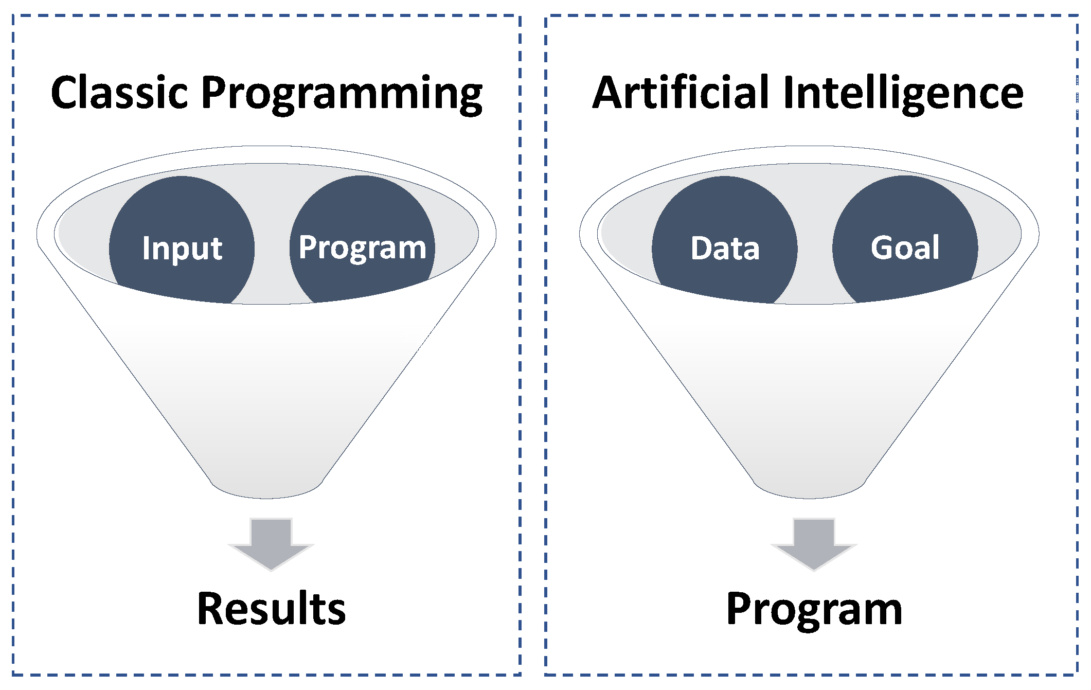
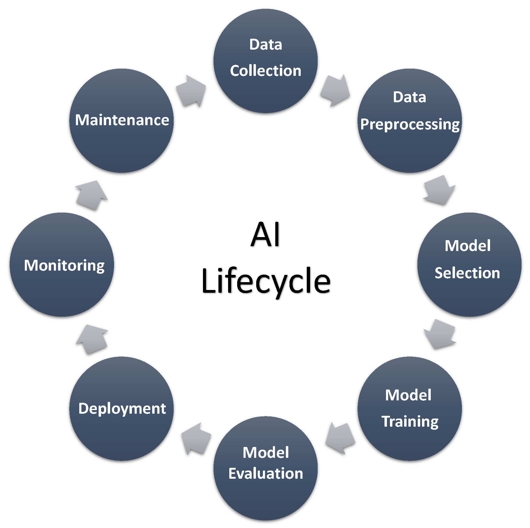
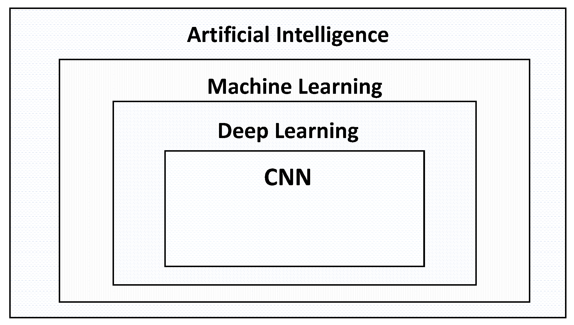
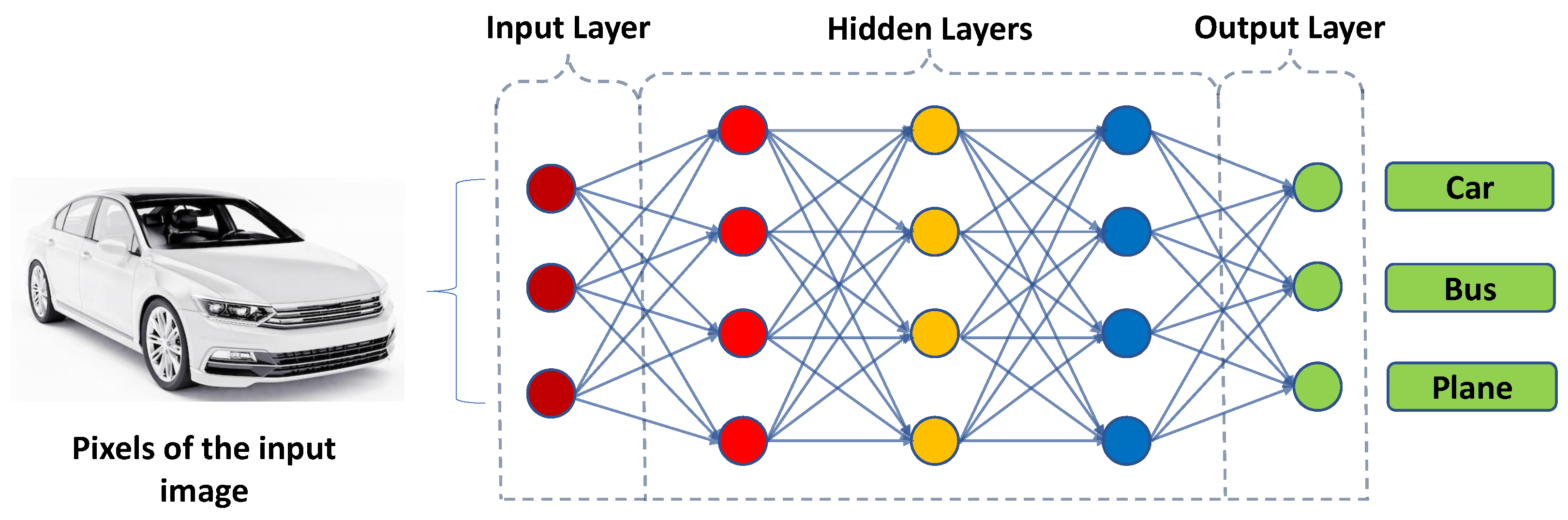
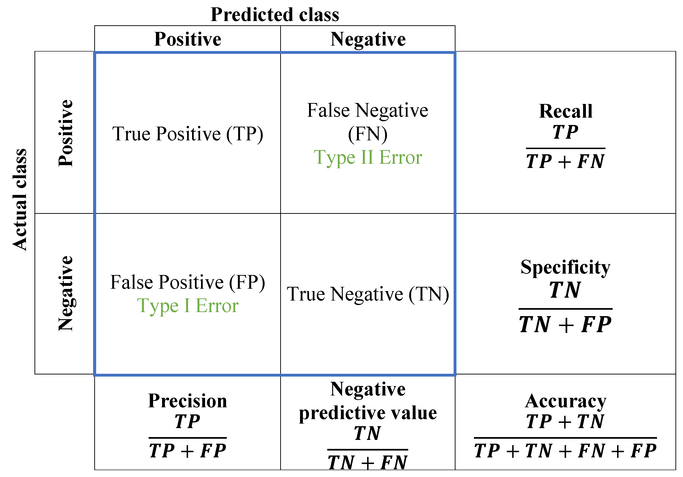
Table 1.
Layers of CNNs and their functions.
| Layer | Function |
|---|---|
| Convolutional layer | Performs a convolution operation on the input image with a set of learnable filters to produce a set of feature maps |
| Pooling layer | Reduces the spatial dimensions of the feature maps produced by the convolutional layer by taking the maximum or average value of non-overlapping regions |
| Activation layer | Applies a non-linear activation function to the output of the previous layer to introduce non-linearity into the network |
| Batch normalization layer | Normalizes the output of the previous layer by subtracting the mean and dividing by the standard deviation of the batch to reduce internal covariate shift and improve convergence |
| Dropout layer | Randomly drops out a percentage of the neurons in the previous layer during training to prevent overfitting and force the network to learn more robust features |
| Fully connected layer | Connects every neuron in the previous layer to every neuron in the current layer, typically used at the end of the network to produce the final output |
| Recurrent layer (specialized) | Captures temporal dependencies in the input sequence, used in recurrent CNN (RCNN) |
| ine LSTM layer (specialized) | Learns long-term dependencies in the input sequence, used in long short-term memory (LSTM) CNN |
Table 2.
Optimization algorithms for CNNs.
| Optimization Algorithm | Description |
|---|---|
| SGD | Updates weights and biases based on gradient of Loss_Func |
| Momentum | Adds a momentum term to smooth out updates and accelerate convergence |
| AdaGrad | Adapts learning rate for each weight based on magnitude of gradients seen so far |
| RMSProp | Uses a moving average of squared gradients to adapt learning rate for each weight |
| Adam | Combines ideas from momentum and AdaGrad to create an adaptive learning rate algorithm |
Table 3.
Regularization techniques for preventing overfitting in CNNs.
| Regularization Technique | Description |
|---|---|
| L1 regularization | Adds a penalty to the Loss_Func proportional to the absolute value of the weights to encourage sparsity and feature selection |
| L2 regularization | Adds a penalty to the Loss_Func proportional to the square of the weights to encourage small weights and prevent overfitting |
| Dropout | Randomly drops out some of the neurons in the network during training to prevent over-reliance on any one feature and improve generalization performance |
| Early stopping | Stops the training process early based on a validation set performance metric to prevent overfitting to the training data |
Table 4.
Comparison of CNN Architectures.
| Architecture | Year | Layers | Filters | Top-1 Error | Top-5 Error |
|---|---|---|---|---|---|
| LeNet | 1998 | 5 | 6–16 | N/A | N/A |
| AlexNet | 2012 | 8 | 96–512 | 37.5% | 17.0% |
| VGG | 2014 | 19 | 64–512 | 27.0% | 8.7% |
| ResNet | 2015 | 152 | 64–512 | 3.6% | 1.6% |
| InceptionNet | 2014 | 22 | 64–512 | 6.7% | 1.9% |
Table 5.
Some examples of the use of CNNs.
| Paper | Summary |
|---|---|
| [149] | Automated method for detecting multi-class welding faults in X-ray pictures using data augmentation and a CNN, achieving 92% accuracy rate. |
| [150] | Developed a novel dataset and machine-learning-based VSR technique for Kannada, achieving 91.90% accuracy. |
| [151] | Developed a novel deep ensemble learning technique for olive leaf disease detection and classification, achieving 96% multi-class classification accuracy and 97% binary classification accuracy. |
| [105] | Developed a computer-vision-based mask recognition algorithm for COVID-19, achieving high accuracy rates. |
| [152] | Proposed using DCNNs and transfer-learning-based pre-trained CNN models to improve visual spam categorization, achieving up to 99% accuracy. |
| [153] | Developed a lightweight CNN-based model for driver sleepiness detection, achieving high accuracy rates and suitable for embedded systems and Android devices. |
Table 6.
Advantages and limitations of CNNs.
| Advantages | Limitations |
|---|---|
| Learn hierarchical representations of input data | Require large amount of labeled training data |
| Handle inputs of varying sizes and aspect ratios | Sensitive to quality of training data |
| Generalize well to new data | Computationally expensive to train and evaluate |
| Allow transfer learning to improve accuracy and reduce training data required | Require significant variation in data to avoid overfitting |
Table 7.
Comparison of platforms and libraries for building CNNs.
| Platform/Library | Ease of Use | Flexibility | Efficiency | Pre-Trained Models |
|---|---|---|---|---|
| TensorFlow | Medium | High | High | Yes |
| Keras | High | Low | Medium | Yes |
| PyTorch | High | High | Medium | Yes |
| Caffe | Low | Low | High | Yes |
| MXNet | Medium | High | High | Yes |
Table 8.
Comparison of model architectures.
| Model Architecture | Visual Data | Sequential Data | Graph Data | Symbolic Data |
|---|---|---|---|---|
| CNNs | Best | Good | Poor | Poor |
| Fully Connected NNs | Poor | Good | Poor | Poor |
| Recurrent NNs | Poor | Best | Poor | Poor |
| Graph NNs | Poor | Poor | Best | Poor |
| Rule-based systems | Poor | Poor | Poor | Best |
Table 9.
Recommendations for building and training CNNs.
| Recommendation | Description |
|---|---|
| Preprocessing the data | Transform the raw input data into a format that can be utilized by the CNN, including resizing images, normalizing pixel values, and augmenting the data to improve accuracy and generalization. |
| Choosing appropriate Hyper_Param | Tune Hyper_Param such as learning rate, batch size, and number of epochs using techniques such as grid search or random search. Avoid overfitting by using techniques such as early stopping or reducing the learning rate over time. |
| Using regularization techniques | Use techniques such as L1 or L2 regularization, dropout, or batch normalization to prevent overfitting and improve the generalization of the model. |
| Hardware considerations | Choose hardware that can handle the computational requirements of the model, use distributed training to train large models on multiple machines in parallel, and optimize memory usage and batch size for efficiency. |
| Evaluating model performance | Split the data into training, validation, and testing sets, use metrics such as accuracy, precision, recall, and F1 score to evaluate the performance of the model, and consider the potential biases and ethical implications of the model. |
| Security aspects | Ensure that the data utilized to train the model is anonymized and that proper measures are taken to protect the privacy and security of the data. Protect against adversarial examples and model poisoning attacks, and ensure that appropriate policies and regulations are in place to govern the use of CNNs. |
Table 10.
Recent developments in CNNs.
| Innovation | Description |
|---|---|
| Attention Mechanisms | A tool for selectively focusing on specific regions of an image or sequence of data, rather than processing the entire input at once, which can improve accuracy and reduce computational requirements. |
| Capsule Networks | A technique for representing objects as capsules, which capture the properties of the object, resulting in a more robust representation of the input data. |
| Transfer Learning | A technique for leveraging the knowledge learned from one task to improve performance on a second, related task, particularly when training data for the second task is limited or unavailable. |
| Adversarial Training | A technique for improving the robustness of CNNs to adversarial attacks by training the model on both the original, clean dataset and a modified version of the dataset that includes adversarial examples. |
| Quantization and Compression | Techniques for reducing the memory and computational requirements of CNNs by representing the weights and activations of the model using fewer bits or by pruning unnecessary weights or neurons. |
Table 11.
Benefits of using formal methods to enhance reliability and efficiency of CNNs.
| Benefits of Using Formal Methods | Description |
|---|---|
| Verification of model specifications | Ensures accuracy, efficiency, and robustness of the model |
| Generation of adversarial examples | Evaluates the robustness of the model and identifies potential vulnerabilities |
| Optimization of Hyper_Param configurations | Identifies the optimal configuration that meets the desired specifications and requirements |
| Development of automated tools | Reduces time and effort required for designing and verifying CNNs, while improving the reliability and quality of the models |
Disclaimer/Publisher’s Note: The statements, opinions and data contained in all publications are solely those of the individual author(s) and contributor(s) and not of MDPI and/or the editor(s). MDPI and/or the editor(s) disclaim responsibility for any injury to people or property resulting from any ideas, methods, instructions or products referred to in the content. |
© 2023 by the author. Licensee MDPI, Basel, Switzerland. This article is an open access article distributed under the terms and conditions of the Creative Commons Attribution (CC BY) license (https://creativecommons.org/licenses/by/4.0/).
Share and Cite
MDPI and ACS Style
Krichen, M. Convolutional Neural Networks: A Survey. Computers 2023, 12, 151. https://doi.org/10.3390/computers12080151
AMA Style
Krichen M. Convolutional Neural Networks: A Survey. Computers. 2023; 12(8):151. https://doi.org/10.3390/computers12080151
Chicago/Turabian StyleKrichen, Moez. 2023. "Convolutional Neural Networks: A Survey" Computers 12, no. 8: 151. https://doi.org/10.3390/computers12080151
Note that from the first issue of 2016, this journal uses article numbers instead of page numbers. See further details here.