Applying Bounding Techniques on Grammatical Evolution

Abstract

The Grammatical Evolution technique has been successfully applied to some datasets from various scientific fields. However, in Grammatical Evolution, the chromosomes can be initialized at wide value intervals, which can lead to a decrease in the efficiency of the underlying technique. In this paper, a technique for discovering appropriate intervals for the initialization of chromosomes is proposed using partition rules guided by a genetic algorithm. This method has been applied to feature construction techniques used in a variety of scientific papers. After successfully finding a promising interval, the feature construction technique is applied and the chromosomes are initialized within that interval. This technique was applied to a number of known problems in the relevant literature, and the results are extremely promising.

1. Introduction

The method of genetic algorithms was proposed by John Holland in the related work in [1]. These algorithms are considered a special case of evolutionary techniques, in which a group of candidate solutions (called also chromosomes) of any optimization problem are evolved iteratively by applying procedures based on natural processes, such as selection, crossover, and mutation [2,3,4]. Usually, chromosomes are arrays of decimal numbers that represent some possible solution to an optimization problem. A special case of genetic algorithms is Grammatical Evolution [5], where the chromosomes are a series of integer values. The genes of a chromosome in Grammatical Evolution stand for production rules of a given Backus–Naur form (BNF) prototype [6]. This process can be used to construct programs to the provided language described by the BNF grammar. This method has been used in many cases, such as function regression problems [7,8], credit classification [9], intrusion detection in computer networks [10], monitoring of water quality [11], mathematical problems [12], composition of music [13], the construction of neural networks [14,15], producing numeric constants [16], computer games [17,18], estimation of energy consumption [19], combinatorial optimization [20], cryptography [21], the production of decision trees [22], automatic circuit design [23], etc.

A number of extensions have been proposed in recent years by a number of researchers on Grammatical Evolution, such as Structured Grammatical Evolution [24,25], which utilizes one-to-one mapping between the values of the chromosomes and the nonterminal symbols of the grammar, incorporation of Particle Swarm Optimization (PSO) [26] to generate programs with Grammatical Evolution, denoted as Grammatical Swarm [27,28], the application of parallel programming techniques to Grammatical Evolution [29,30], etc. Furthermore, a series of software have been developed for Grammatical Evolution, such as the GEVA [31], which utilizes the Java programming language to implement various problems for Grammatical Evolution, and it also provides a simple GUI to control the evolutionary process, the gramEvol software [32], which provides a package in the R programming language, the GeLab [33], which implements a Matlab toolbox for Grammatical Evolution, the GenClass [34] software used to produce artificial classification programs in a C-like language, the QFc software [35] used to construct artificial feature for classification and regression problems, etc. These artificial features can be considered as functions of the initial features, and in most cases, these features are fewer in number than the original.

An important issue of the Grammatical Evolution technique is that usually, the integer chromosomes take values in a large interval of values, e.g., $\left[0\dots 255\right]$, as a result of which there is a significant delay in finding the most suitable programs, as many of the values in the above interval are not used. Furthermore, in many cases, the performance of Grammatical Evolution is not as expected, and numerous chromosomes and/or generations are required to estimate the most appropriate program. The present work proposes a two-step technique to tackle the above problem. In the first step of the proposed technique, the value limits for the genes of the chromosomes are estimated using a genetic algorithm, and a similar approach as in [36], and in the second stage, the Grammatical Evolution chromosomes are initialized within the best value interval of the first stage. The purpose of this technique is to identify an interval of values for the gene values within which the search for the global minimum of the objective problem will be most efficient. This technique starts from a wide range of values, which is gradually narrowed until a promising configuration is identified. The proposed approach was tested in the feature construction procedure, initially suggested in [37]. This procedure for feature construction has also been used in many problems, such as the identification of spam emails [38], medical problems [39], signal processing of EEG signals [40,41], etc. The usage of the proposed interval technique in the construction of features significantly increased the performance of the method, both in classification problems and in regression problems, as is provided in the Experiments Section. However, the proposed interval technique is quite general and can be applied to other problems dealt with by Grammatical Evolution.

The remainder of this paper has the following structure: Section 2 discusses in detail the proposed method, Section 3 lists the datasets used in the experimental results and the experimental results, and finally, Section 4 provides some conclusions and guidelines for future research.

2. The Proposed Method

2.1. Preliminaries

The Grammatical Evolution employs chromosomes that stand for a series of production rules of the provided BNF grammar. The tuple $G=\left(N,T,S,P\right)$ defines any BNF grammar, where the following holds:

• N is a set that contains the nonterminal symbols of the grammar.
• T is a set that contains the terminal symbols.
• The nonterminal symbol S denotes the start symbol of the grammar, from which the production will initiate.
• P is a set that contains the production rules of the grammar.

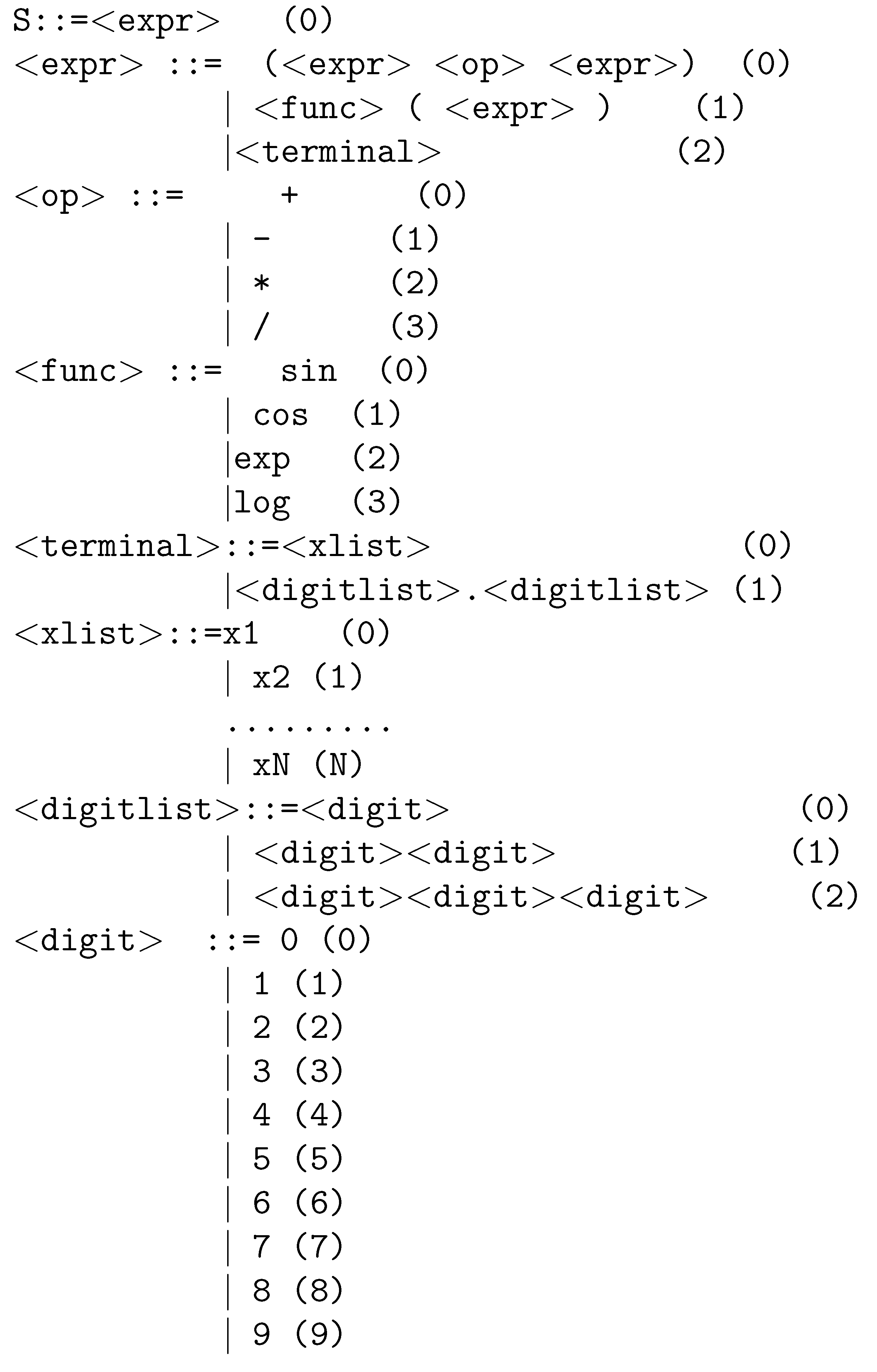
The original BNF grammar is extended by enumerating the production rules. For each nonterminal symbol, the production rules are given a sequence number starting from 0, which will help the Grammatical Evolution process in choosing the next production rule. As a full working example, consider the extended BNF grammar shown in Figure 1. The nonterminal symbols are enclosed in the <> symbols. The sequence numbers of the production rules are inside the parentheses of the extended grammar. The constant N denotes the dimension of the input data. The production of valid programs initiates from the start symbol of the grammar and through a series of steps creates a program by substituting non terminal symbols with the right hand of the considered production rule. The selection of each production rule is performed using the following steps:

• Obtain the next gene V from the current chromosome.
• The next production rule is selected using the scheme Rule = V mod NR. The number NR represents the total number of production rules for under processing the non terminal symbol.

For example, consider the following chromosome:

$$x=\left[9,8,6,4,16,10,17,23,8,14\right]$$

with $N=3$. The constant N denotes the number of initial features in the used dataset. The expression $f\left(x\right)=x_2+cos\left(x_3\right)$ is produced through the steps shown in

Table 1. This table indicates the steps executed to construct a program using the mentioned grammar.

Expression	Chromosome	Selected Operation
<expr>	9, 8, 6, 4, 16, 10, 17, 23, 8, 14	$9mod3=0$
(<expr><op><expr>)	8, 6, 4, 16, 10, 17, 23, 8, 14	$8mod3=2$
(<terminal><op><expr>)	6, 4, 16, 10, 17, 23, 8, 14	$6mod2=0$
(<xlist><op><expr>)	4, 16, 10, 17, 23, 8, 14	$4mod3=1$
(x2<op><expr>)	16, 10, 17, 23, 8, 14	$16mod4=0$
(x2+<expr>)	10, 17, 23, 8, 14	$10mod3=1$
(x2+<func>(<expr>))	17, 23, 8, 14	$17mod4=1$
(x2+cos(<expr>))	23, 8, 14	$23mod2=2$
(x2+cos(<terminal>))	8, 14	$8mod2=0$
(x2+cos(<xlist>))	14	$14mod3=2$
(x2+cos(x3))

. This transformation of the initial 3 features of a hypothetical problem into just 1 artificial feature also shows the dynamics of the feature construction method, since with its use there can be a dramatic reduction in the dimension of the objective problem while preserving all the necessary information.

2.2. The Feature Construction Method

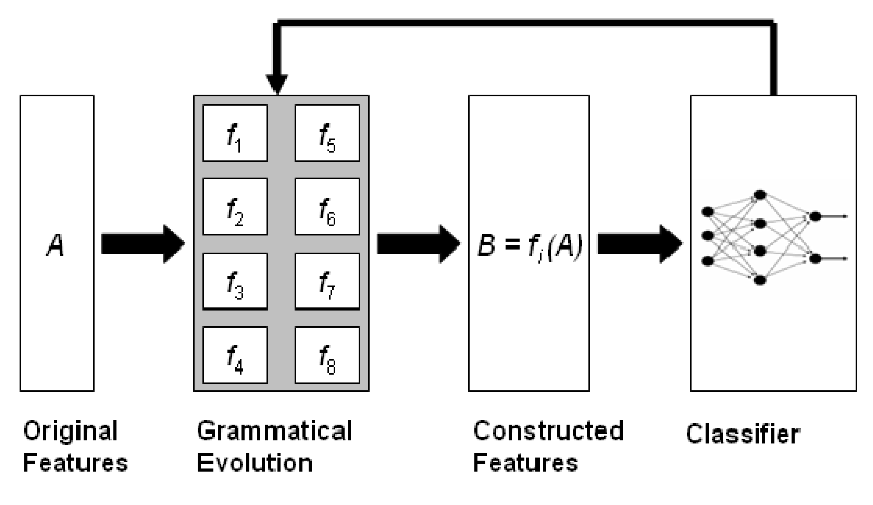
The feature construction method constructs new features from the initial using the Grammatical Evolution procedure, and the main steps are graphically illustrated in Figure 2.

This process creates artificial features which are evaluated using a machine learning technique, such as an artificial neural network [42,43] or a Radial Basis Function (RBF) network [44,45]. In order to speed up the process, the RBF network is used in the current work. The main steps of the process are as follows:

1.

Initialization step.

(a)

Obtain the train dataset of the objective problem. This dataset is considered as a series of M pairs $\left(x_i,t_i\right),i=1,\dots ,M$, where $t_i$ denotes the expected output for the vector $x_i$.

(b)

Set the parameters of the method: $N_G$ as the number of allowed generations,  $N_C$ as the total number of chromosomes, $p_s$ as the selection rate, and  $p_m$ as the mutation rate.

(c)

Define as $N_f$ the number of features that will be constructed.

(d)

Initialize the chromosomes. Every gene of each chromosome is considered a positive random integer.

(e)

Set iter = 1

2.

Genetic step

(a)

For $i=1,\dots ,N_G$ do

i.

Produce with the Grammatical Evolution given in Section 2.1, a set of $N_f$ artificial features for the chromosome $g_i$.

ii.

Execute a transformation of the original features using the set of features created previously. Denote the new train set as $\left(x_{g_i,j},t_j\right),j=1,\dots ,M$

iii.

Apply a machine learning model C on the new dataset and train the model C. The output value of this model is defined as $C\left(x\right)$. The fitness $f_i$ is calculated as follows:

$$f_i=\sum _{j=1}^M{\left(C\left(x_{g_i,j}\right)-t_j\right)}^2$$

(1)

This equation defines the training error of model C for the modified train set $\left(x_{g_i,j},t_j\right),j=1,\dots ,M$. This fitness function can be thought of as a performance measure of using the artificial features produced by Grammatical Evolution. The most promising features will have a lower price than the worst features.

iv.

Perform the selection procedure, where initially the chromosomes are sorted according to their fitness. The first  $\left(1-p_s\right)\times N_C$ chromosomes are copied to the next generation. The remaining chromosomes will be substituted by offsprings produced during the crossover procedure.

v.

Perform the crossover procedure. This process will create $p_s\times N_c$ offsprings. Initially, two distinct chromosomes are selected for every pair of constructed offsprings. The selection is performed using the tournament selection. The procedure of tournament selection has the following steps: Randomly create a set of $T_s>1$ chromosomes and select as a parent from this set the chromosome with the lowest fitness value. For each pair of $(z,w)$ parents, two offsprings $\tilde{z}$ and $\tilde{w}$ are produced utilizing the so-called one-point crossover, which is graphically demonstrated in Figure 3. This crossover method was also used in the original paper of the Grammatical Evolution technique [5]. As an example, consider the chromosome

$$x=\left[9,8,6,4,16,10,17,23,8,14\right]$$

shown in the previous subsection, and the chromosome

$$y=[10,9,2,5,4,3,7,8,10,12]$$

The chromosome x produces the expression $f_1\left(x\right)=x_2+cos\left(x_3\right)$ and the chromosome y produces the expression $f_2\left(x\right)=sin\left(x_1\right)$ using the grammar of Figure 1 and $N=3$. If position 3 is selected as the cutting point for the one-point crossover procedure, then the offspring

$$z=\left[10,9,2,4,16,10,17,23,8,14\right]$$

and the valid expression $f_3\left(x\right)=cos\left(x_2\right)$ will be produced using the grammar of Figure 1.

vi.

Perform the mutation procedure. For each element of every chromosome, a random number $r\in \left[0,1\right]$ is selected. The corresponding element is altered if $r\le p_m$. In most cases of genetic algorithms, the mutation rate takes small values, e.g., 1–5%, in order for random changes to occur in the chromosomes, on the one hand, leading the optimization to search for the total minimum, but on the other hand, not to lose good values that have been discovered in some generation of the algorithm. As an example of the mutation procedure, consider the chromosome

$$x=\left[9,8,6,4,16,10,17,23,8,14\right]$$

used in the previous subsection that constructs the artificial feature $f\left(x\right)=x_2+cos\left(x_3\right)$. If the mutation procedure alters the value 17 to 16, the new chromosome will be the following:

$$x^{\prime }=\left[9,8,6,4,16,10,16,23,8,14\right]$$

and subsequently, the new feature will be $f\left(x\right)=x_2+sin\left(x_3\right)$

(b)

EndFor

3.

Set iter=iter+1

4.

If $\mathrm{iter}\le N_G$ goto Genetic Step, else the process is terminated and the best chromosome $g^{*}$ is obtained.

5.

Apply the $N_f$ features that correspond to $g^{*}$ to the test set.

6.

Apply a machine learning model to the new test set and obtain the corresponding test error.

2.3. The Proposed Method

In the present technique, a procedure is conducted before the initialization of the chromosomes of the algorithm described in Section 2.2. This process, using a modified genetic algorithm, aims to find the optimal value interval for the genes. In the current work, the chromosomes are sets of intervals, as well as the fitness values. Hence, a comparison operator should be used in order to compare intervals. In order to compare the intervals $a=\left[a_1,a_2\right]$, $b=\left[b_1,b_2\right]$, the operator is $L^{*}(a,b)$ used defined as:

$$\begin{array}{ccc}\hfill L^{*}(a,b)& =& \left\{\begin{array}{cc}\mathrm{TRUE},\hfill & a_1<b_1,\mathrm{OR}\left(a_1=b_1\mathrm{AND}{a}_2<b_2\right)\hfill \\ \mathrm{FALSE},\hfill & \mathrm{OTHERWISE}\hfill \end{array}\right.\hfill \end{array}$$

(2)

The steps of the proposed method are listed in Algorithm 1.

Algorithm 1 The steps of the main procedure used to discover the optimal value interval.

1. Initialization Step (a) Set as  $I_C$ the total number of chromosomes, $I_G$ the number of generations,  $p_s$ the selection rate, and $p_m$ the mutation rate. Also, define as $I_M$ the initial margin. This integer value determines the maximum value that the genes of the chromosome can take. Gradually, the algorithm will generate tighter bounds for gene values. (b) Construct the initial set $N_M$ of margins $$N_M={\left[0,I_M\right]}^{\left(n\right)}$$ (3) where n is the number of genes for the chromosomes of the Grammatical Evolution procedure. This set defines for each gene the interval of values in which it can be initialized. (c) Initialize a genetic population of $I_C$ chromosomes. Every chromosome contains a set for intervals randomly initialized in $N_M$. An Example of a chromosome with $n=5$ can be the following: $\left[\left(0,12\right),\left(0,30\right),\left(0,21\right),\left(0,100\right),\left(0,192\right)\right]$. This interval will be used as the initial value interval for the genes of the chromosome. Progressively, the above interval will be adjusted and its range reduced in order to improve the performance of the process controlled by Grammatical Evolution. (d) Set iter = 0 2. Evaluation Step (a) For $i=1,\dots ,I_C$ do i. Create $N_S$ random sets of intervals inside the range defined by chromosome $g_i$. ii. Execute the procedure of Section 2.2, by initializing the chromosomes of the Grammatical Evolution procedure inside set every random set. iii. Denote by $E_{min}\left(g_i\right)$ the minimum train error obtained by the feature construction procedure. iv. Denote by $E_{max}\left(g_i\right)$ the maximum train error obtained by the feature construction procedure. v. Set $f_i=\left[E_{min}\left(g_i\right),E_{max}\left(g_i\right)\right]$, as the fitness value of chromosome $g_i$. Fitness is represented as the range of values between the best and worst value for the chromosome under consideration. Gradually, the genetic algorithm will find lower values for the left end of the value interval while trying to reduce the range of that interval. To achieve interval comparison, it uses the operator L, introduced in Equation (2). This way, it will find the optimal set of values for the initialization of the chromosomes. 3. EndFor 4. Genetic step (a) Perform the crossover procedure of Algorithm 2. (b) Perform the mutation procedure of Algorithm 3. 5. Termination Check Step (a) Set  $iter=iter+1$ (b) If $iter>I_G$, then Terminate and report the chromosome $g_{\mathrm{best}}$ with the best fitness, else Goto Evaluation Step. (c) Endif

Algorithm 2 The steps of the crossover procedure used in the current method.

1. The chromosomes are sorted with respect to their fitness values. 2. The first $\left(1-p_s\right)\times I_c$ chromosomes are copied intact to the next generation and the rest of the population is replaced by offsprings created. 3. For each pair of offsprings, two chromosomes $z=\left(z_1,z_2,\dots ,z_n\right),y=\left(y_1,y_2,\dots ,y_n\right)$ are selected by utilizing the procedure of tournament selection with tournament size $T_s$. For each value of the offsprings $\tilde{z}$ and $\tilde{y}$, with $i=1,\dots ,n$, the following operation is executed: $$\begin{array}{ccc}\hfill \widetilde{z_i}& =& a_i{z}_i+\left(1-a_i\right)y_i\hfill \\ \hfill \widetilde{y_i}& =& a_i{y}_i+\left(1-a_i\right)z_i\hfill \end{array}$$ (4) The value $a_i$ is a random number in $[-0.5,1.5]$. This process and the range of $a_i$ random values are suggested in [46].

Algorithm 3 Mutation procedure for current work.

1. For each chromosome g Do (a) For every gene $g_i,i=1,\dots ,n$ Do Draw a random number $r\in [0,1]$ If $r<p_m$ then $g_i=\mathrm{left}\left(g_i\right)+z\left(\mathrm{right}\left(g_i\right)-\mathrm{left}\left(g_i\right)\right)$, where z is a random number in $[0,1]$. The function left(x) represents the lower value of the interval x, and the function right(x) represents the upper value of the interval x. (b) EndFor 2. EndFor

3. Experiments

The present methodology was applied to a number of datasets from fields and the method was compared with other techniques used in the bibliography. The datasets used to run the experiments are freely available at the following websites:

1.

The UCI dataset repository, https://archive.ics.uci.edu/ml/index.php (accessed on 18 February 2024) [47].

2.

The Keel repository, https://sci2s.ugr.es/keel/datasets.php (accessed on 18 February 2024) [48].

3.

The Statlib library located in http://lib.stat.cmu.edu/datasets/ (accessed on 18 February 2024).

3.1. Classification Datasets

The list of classification datasets is as follows:

1.

Appendictis, a medical dataset used in [49].

2.

Australian dataset [50], which is about credit card transactions.

3.

Balance dataset [51], which is a dataset used in psychological experiments.

4.

Circular dataset: An artificial dataset that contains 1000 examples which belong to two categories (500 examples each).

5.

Cleveland dataset: A medical dataset that has been employed in a variety of scientific papers [52,53].

6.

Dermatology dataset [54]: A medical dataset about dermatological deceases.

7.

Haberman dataset: A medical dataset about breast cancer.

8.

Heart dataset [55]: A medical dataset related to heart diseases.

9.

Hayes roth dataset [56].

10.

HouseVotes dataset [57]: A statistical dataset created from the votes in the U.S. House of Representatives Congressmen.

11.

Ionosphere dataset: It was used in experiments related to the ionosphere [58,59].

12.

Liverdisorder dataset [60]: A medical dataset.

13.

Mammographic dataset [61]: A medical dataset related to breast cancer.

14.

Parkinsons dataset: A medical dataset related to Parkinson’s disease (PD) [62].

15.

Pima dataset [63]: A medical dataset related to the diabetes presence.

16.

Popfailures dataset [64]: A dataset related to climate experiments.

17.

Regions2 dataset: A medical dataset about the presence of hepatitis C [65].

18.

Saheart dataset [66]: A dataset related to heart deceases.

19.

Segment dataset [67]: Represents an image processing dataset.

20.

Spiral dataset, which is a dataset with two categories.

21.

Student dataset [68]: An education dataset.

22.

Transfusion dataset [69]: Data taken from the Blood Transfusion Service Center in Hsin-Chu City in Taiwan.

23.

Wdbc dataset [70], A medical dataset related to cancer.

24.

Wine dataset, which is used in various papers [71,72] to obtain the quality of wines.

25.

Eeg datasets: A medical dataset about EEG signals [73]. For this dataset, the following cases were considered: Z_F_S, Z_O_N_F_S, ZO_NF_S, and ZONF_S.

26.

Zoo dataset [74]: Related to animal classification.

The number of classes for each classification dataset is shown in

Table 2. Number of classes for each classification dataset.

Dataset	Classes
Appendicitis	2
Australian	2
Balance	3
Circular	2
Cleveland	5
Dermatology	6
Haberman	2
Hayes Roth	3
Heart	2
Housevotes	2
Ionosphere	2
Liverdisorder	2
Mammographic	2
Parkinsons	2
Pima	2
Popfailures	2
Regions2	5
Saheart	2
Segment	7
Spiral	2
Student	4
Transfusion	2
Wdbc	2
Wine	3
Z_F_S	3
Z_O_N_F_S	5
ZO_NF_S	3
ZONF_S	2
Zoo	7

.

3.2. Regression Datasets

The following regression datasets were used:

• Abalone dataset [75]: A dataset related to the prediction of the age of abalones.
• Airfoil dataset: Used by NASA [76].
• Baseball dataset: It was used to predict the financial earnings of baseball players.
• Concrete dataset [77]: A dataset related to civil engineering.
• Dee dataset: Used to predict the price of electricity.
• ELE dataset: Electrical length dataset downloaded from the KEEL repository.
• HO dataset: Downloaded from the STALIB repository.
• Housing dataset: Provided in [78].
• Laser dataset: Stands for data collected during laser experiments.
• LW dataset: This dataset is produced from a study to identify risk factors associated with low-weight babies.
• MORTGAGE dataset: A dataset related to economic measurements from the USA.
• PL dataset: Downloaded from the STALIB repository.
• SN dataset: Downloaded from the STALIB repository.
• Treasury dataset: A dataset related to economic measurements from the USA.
• TZ dataset: Downloaded from the STALIB repository.

3.3. Experimental Results

All the methods utilized in the experiments were coded in ANSI C++ (gcc version 13.2.0) using the freely available optimization package of OPTIMUS, which is available from https://github.com/itsoulos/OPTIMUS/ (accessed on 19 April 2024). The series of experiments were executed 30 times. In every execution, a different initialization for the random numbers was used, and the function drand48() of C++ was used to produce random numbers. The validation of the conducted experiments was performed using a 10-fold validation method. This method has been utilized in many research papers, and it is considered as a standard validation method. In the event that small datasets are provided, other validation techniques may be used, such as the leave-one-out method. The average classification error measured on the test set is reported for the classification datasets and the average regression error for the regression datasets. The values for the experimental parameters are shown in

Table 3. The values for the parameters used in the conducted experiments.

Name	Purpose	Value
$N_C$	Number of chromosomes	500
$N_G$	Number of generations	200
$p_s$	Selection rate	0.10
$p_m$	Mutation rate	0.05
$T_s$	Tournament size	8
$N_f$	Number of features	2
H	Number of hidden nodes	10
$I_C$	Number of chromosomes (proposed method)	200
$I_G$	Number of generations (proposed method)	10
$I_M$	Initial right bound (proposed method)	1024

. The results are listed in

Table 4. Experimental results using the series of machine learning models on classification datasets. The numbers in cells represents the average classification error that was calculated on the test set.

DATASET	ADAM	NEAT	MLP	RBF	FC	IFC10	IFC20
APPENDICITIS	16.50%	17.20%	18.10%	12.23%	15.86%	16.18%	15.94%
AUSTRALIAN	35.65%	31.98%	32.21%	34.89%	16.48%	13.80%	14.05%
BALANCE	7.87%	23.84%	8.97%	33.42%	11.16%	0.38%	0.00%
CIRCULAR	3.94%	34.07%	5.99%	6.30%	3.69%	3.27%	3.04%
CLEVELAND	67.55%	53.44%	51.60%	67.10%	47.74%	44.79%	44.86%
DERMATOLOGY	26.14%	32.43%	30.58%	62.34%	27.47%	11.23%	13.43%
HABERMAN	29.00%	24.04%	28.66%	25.10%	26.62%	23.03%	22.94%
HAYES ROTH	59.70%	50.15%	56.18%	64.36%	32.70%	18.50%	16.96%
HEART	38.53%	39.27%	28.34%	31.20%	18.13%	15.08%	15.53%
HOUSEVOTES	7.48%	10.89%	6.62%	6.13%	11.20%	6.77%	8.09%
IONOSPHERE	16.64%	19.67%	15.14%	16.22%	10.09%	9.83%	11.38%
LIVERDISORDER	41.53%	30.67%	31.11%	30.84%	31.01%	28.93%	30.03%
MAMMOGRAPHIC	46.25%	22.85%	19.88%	21.38%	16.77%	14.91%	14.72%
PARKINSONS	24.06%	18.56%	18.05%	17.41%	10.60%	11.09%	9.39%
PIMA	34.85%	34.51%	32.19%	25.78%	24.43%	23.26%	24.12%
POPFAILURES	5.18%	7.05%	5.94%	7.04%	5.33%	4.78%	4.64%
REGIONS2	29.85%	33.23%	29.39%	38.29%	29.69%	26.38%	26.58%
SAHEART	34.04%	34.51%	34.86%	32.19%	29.45%	29.40%	29.93%
SEGMENT	49.75%	66.72%	57.72%	59.68%	47.81%	31.19%	30.27%
SPIRAL	43.42%	48.66%	40.21%	44.87%	31.69%	26.06%	22.41%
STUDENT	5.13%	12.50%	5.61%	7.52%	5.29%	3.57%	3.61%
TRANSFUSION	25.68%	24.87%	25.84%	27.36%	22.54%	19.99%	20.76%
WDBC	35.35%	12.88%	8.56%	7.27%	3.66%	3.42%	2.52%
WINE	29.40%	25.43%	19.20%	31.41%	7.49%	7.97%	8.92%
Z_F_S	47.81%	38.41%	10.73%	13.16%	5.31%	6.01%	5.37%
Z_O_N_F_S	78.79%	79.08%	64.81%	60.40%	37.97%	32.78%	32.23%
ZO_NF_S	47.43%	43.75%	8.41%	9.02%	4.74%	4.04%	4.22%
ZONF_S	11.99%	5.44%	2.60%	4.03%	2.66%	2.49%	2.24%
ZOO	14.13%	20.27%	16.67%	21.93%	25.33%	11.32%	10.40%
AVERAGE	31.50%	30.91%	24.10%	27.86%	19.31%	15.53%	15.47%

and

Table 5. Experimental results using the series of machine learning models on regression datasets. The numbers in cells represents the average regression error that was calculated on the test set.

DATASET	ADAM	NEAT	MLP	RBF	FC	IFC10	IFC20
ABALONE	4.30	9.88	7.17	7.37	4.66	3.73	3.70
AIRFOIL	0.005	0.067	0.003	0.27	0.002	0.001	0.001
BASEBALL	77.90	100.39	103.60	93.02	71.45	55.64	56.91
CONCRETE	0.078	0.081	0.0099	0.011	0.006	0.005	0.005
DEE	0.63	1.512	1.013	0.17	0.17	0.18	0.19
ELE	46.32	79.91	75.06	49.95	43.54	36.60	26.71
HO	0.035	0.167	2.78	0.03	0.009	0.013	0.017
HOUSING	80.20	56.49	43.26	57.68	27.58	13.14	14.60
LASER	0.03	0.084	0.59	0.024	0.009	0.024	0.031
LW	0.028	0.17	1.90	1.14	0.73	0.013	0.015
MORTGAGE	9.24	14.11	2.41	1.45	0.58	0.015	0.014
PL	0.117	0.097	0.28	0.083	0.028	0.019	0.018
SN	0.026	0.174	2.95	0.90	0.79	0.038	0.022
TREASURY	11.16	15.52	2.93	2.02	0.63	0.06	0.05
TZ	0.07	0.097	5.38	4.10	3.41	0.40	0.65
AVERAGE	15.34	18.58	16.20	14.27	9.87	7.13	6.60

for the classification and regression datasets, respectively. The following applies to the tables with the experimental results:

• The column DATASET stands for the name of the used dataset.
• The column ADAM denotes the application of the ADAM optimization method [79] in an artificial neural network with $H=10$ processing nodes.
• The column NEAT stands for the usage of the NEAT method (NeuroEvolution of Augmenting Topologies) [80].
• The column MLP stands for the results obtained by a neural network with $H=10$ processing nodes. This network was trained using a genetic algorithm and the BFGS local optimization method [81]. The parameters used by the genetic algorithm are the same as in the case of feature construction.
• The column RBF stands for the results obtained by an RBF network. The network has $H=10$ hidden nodes.
• The column FC represents the results obtained by the feature construction procedure in Section 2.2 without the proposed modification.
• The column IFC10 stands for the incorporation of the proposed technique with the feature construction technique. The parameter $I_G$ was set to 10.
• The column IFC20 stands for the incorporation of the proposed technique with the feature construction technique. The parameter $I_G$ was set to 20.
• The line AVERAGE denotes the average classification or regression error.

From the experimental results and their careful study, one can deduce that the original feature construction method significantly outperforms simple machine learning techniques in terms of classification error or function approximation error. The feature construction method achieved low errors by creating only two artificial features from the existing ones and thus significantly reduced the required information needed for successful classification or data fitting. In addition, the proposed value interval generation technique (IFC10 or IFC20) significantly improves the feature construction technique, both in classification data and data fitting data. Furthermore, a statistical comparison was performed using a scatter plot, and the results are outlined in Figure 4 for the classification datasets and in Figure 5 for the regression datasets.

The scatter plot (Figure 4) effectively demonstrates the comparative performance of various classification methods in terms of classification error percentage. The methods evaluated are MultiLayer Perceptron (MLP), Radial Basis Function (RBF), the simple feature construction technique (FC), and two variants of the proposed modification, named IFC10 and IFC20, respectively. The FC method shows a lower median classification error compared with both MLP and RBF, with the differences being statistically significant (as indicated by the asterisks). This suggests that the FC method outperforms MLP and RBF in terms of classification accuracy. When comparing FC with IFC10, IFC10 displays a lower median classification error, and the difference is statistically significant, suggesting that IFC10 is an improvement over the standard FC method. Between IFC10 and IFC20, the median classification errors are close, and the lack of asterisks (’ns’ for not significant) between these two methods indicates that the difference in classification error is not statistically significant. This suggests that the critical parameter change from IFC10 to IFC20 does not have a significant impact on classification accuracy.

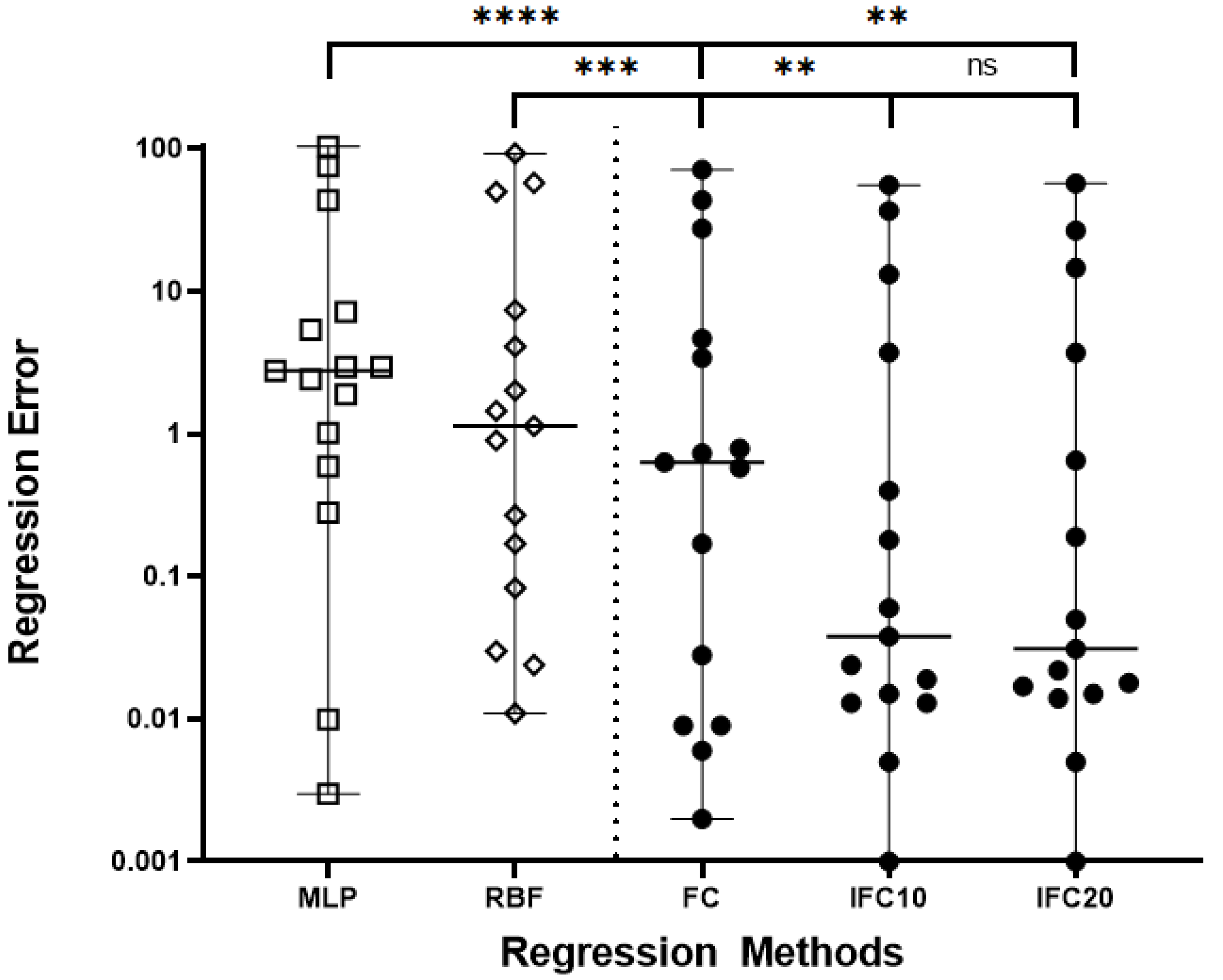
Figure 5 a scatter plot that compares the regression errors among several machine learning regression methods used in our experiments. The plot illustrates the following points, with the inclusion of the Wilcoxon signed-rank test to determine statistical significance: The Feature Construction (FC) method exhibits a lower median regression error compared to both the Multi-Layer Perceptron (MLP) and Radial Basis Function (RBF) methods. The statistical significance of these results is marked by asterisks on the plot: *** indicates a p-value less than 0.001 for the comparison between FC and RBF, and **** indicates a p-value less than 0.0001 for the comparison between FC and MLP. These results substantiate that the FC method significantly outperforms both MLP and RBF in terms of median regression error. When examining the Interval Feature Construction method with the parameter set to 10 (IFC10), we observe a statistically significant reduction in median regression error compared to the FC method, as indicated by ** for a p-value less than 0.01. This denotes a clear improvement with the use of the IFC10 method over the standard FC approach. A comparison between the IFC10 and Interval Feature Construction with the parameter set to 20 (IFC20) reveals a non-significant difference in median regression error, denoted by ’ns’ on the plot. This lack of significance suggests that varying the parameter from 10 to 20 does not result in a statistically significant change in regression error for the IFC method. In conclusion, the FC method demonstrates a significantly better performance compared to traditional methods such as MLP and RBF. The improvement provided by IFC10 over FC is significant, whereas the change in parameters between IFC10 and IFC20 does not yield a significant difference, indicating a plateau in performance gains between these parameter settings.

Also, another experiment was conducted by altering the number of chromosomes in the proposed method from 100 to 500, and the results are outlined in

Table 6. Experiments with the number of chromosomes. Column IFC100 stands for the usage of 100 chromosomes, column IFC200 represents the results for 200 chromosomes, and column IFC500 shows the results for 500 chromosomes.

DATASET	IFC100	IFC200	IFC500
APPENDICITIS	15.19%	16.66%	16.18%
AUSTRALIAN	14.59%	14.24%	13.80%
BALANCE	0.33%	0.97%	0.38%
CIRCULAR	3.21%	3.21%	3.27%
CLEVELAND	43.80%	44.25%	44.79%
DERMATOLOGY	12.16%	14.84%	11.23%
HABERMAN	21.08%	24.93%	23.03%
HAYES ROTH	18.21%	19.41%	18.50%
HEART	15.43%	17.25%	15.08%
HOUSEVOTES	5.59%	6.39%	6.77%
IONOSPHERE	10.72%	10.98%	9.83%
LIVERDISORDER	30.81%	31.34%	28.93%
MAMMOGRAPHIC	15.28%	15.73%	14.91%
PARKINSONS	9.67%	9.77%	11.09%
PIMA	24.74%	24.21%	23.26%
POPFAILURES	5.50%	4.75%	4.78%
REGIONS2	26.16%	26.25%	26.38%
SAHEART	29.67%	29.94%	29.40%
SEGMENT	33.09%	33.58%	31.19%
SPIRAL	26.98%	26.37%	26.06%
STUDENT	4.00%	4.06%	3.57%
TRANSFUSION	22.69%	19.33%	19.99%
WDBC	3.92%	3.61%	3.42%
WINE	9.73%	8.30%	7.97%
Z_F_S	5.22%	5.63%	6.01%
Z_O_N_F_S	34.20%	34.58%	32.78%
ZO_NF_S	4.66%	4.62%	4.04%
ZONF_S	2.44%	2.51%	2.49%
ZOO	9.32%	8.73%	11.32%
AVERAGE	15.81%	16.08%	15.53%

for the classification datasets.

In this experiment, the stability of the proposed technique is revealed, since any changes in the population size do not significantly affect its experimental performance, as measured by the classification error in the test set.

4. Conclusions

In the presented work, a first attempt was made to introduce the concept of intervals into the technique of Grammatical Evolution. With this technique, an attempt was made to find a value interval for the chromosome values that will provide lower values in the objective function to be minimized. For this reason, a genetic algorithm was introduced, which is executed before the main process of Grammatical Evolution and which gradually generates the reliable value interval for the chromosome values. The proposed method will significantly improve the efficiency of the Grammatical Evolution procedure by limiting the optimization to more narrow intervals for the values of the chromosomes.

The method was tested on the feature construction technique, which is guided by Grammatical Evolution. Experimental results and statistical comparison show a significant reduction in classification error and data fitting error using the proposed technique. In addition, from the statistical comparison of the results, it appears that there is no direct effect of the number of generations of the genetic algorithm on the effectiveness of the method, which means that only a few generations are enough to effectively find the promising value interval. Although the proposed technique was applied to the feature generation method, it is quite general, and in the future, it will be possible to apply it to other application areas of Grammatical Evolution, such as the construction of artificial neural networks, the rule generation method, etc. However, a major drawback of the present technique is that it requires a significant amount of computing resources for its execution, but this can be alleviated by using parallel computing techniques, such as the MPI programming library [82] or the OpenMP library [83].

References

- Holland, J.H. Genetic algorithms. Sci. Am. 1992, 267, 66–73. [Google Scholar] [CrossRef]
- Stender, J. Parallel Genetic Algorithms:Theory & Applications; IOS Press: Clifton, VA, USA, 1993. [Google Scholar]
- Goldberg, D. Genetic Algorithms in Search, Optimizatio and Machine Learning; Addison-Wesley Publishing: Reading, MA, USA, 1989. [Google Scholar]
- Michaelewicz, Z. Genetic Algorithms + Data Structures = Evolution Programs; Springer: Berlin/Heidelberg, Germany, 1996. [Google Scholar]
- O’Neill, M.; Ryan, C. Grammatical evolution. IEEE Trans. Evol. Comput. 2011, 5, 349–358. [Google Scholar] [CrossRef]
- Backus, J.W. The Syntax and Semantics of the Proposed International Algebraic Language of the Zurich ACM-GAMM Conference. In Proceedings of the International Conference on Information Processing UNESCO, Paris, France, 15–20 June 1959; pp. 125–132. [Google Scholar]
- Ryan, C.; Collins, J.; O’Neill, M. Grammatical evolution: Evolving programs for an arbitrary language. In Proceedings of the EuroGP 1998, Paris, France, 14–15 April 1998; Springer: Berlin/Heidelberg, Germany, 1998. [Google Scholar]
- O’Neill, M.; Ryan, M.C. Evolving Multi-line Compilable C Programs. In Proceedings of the EuroGP 1999, Goteborg, Sweden, 26–27 May 1999; Springer: Berlin/Heidelberg, Germany, 1999. [Google Scholar]
- Brabazon, A.; O’Neill, M. Credit classification using grammatical evolution. Informatica 2006, 30, 325–335. [Google Scholar]
- Şen, S.; Clark, J.A. A grammatical evolution approach to intrusion detection on mobile ad hoc networks. In Proceedings of the 2nd ACM Conference on Wireless Network Security, Zurich, Switzerland, 16–19 March 2009. [Google Scholar]
- Chen, L.; Tan, C.H.; Kao, S.J.; Wang, T.S. Improvement of remote monitoring on water quality in a subtropical reservoir by incorporating grammatical evolution with parallel genetic algorithms into satellite imagery. Water Res. 2008, 42, 296–306. [Google Scholar] [CrossRef]
- Ryan, C.; O’Neill, M.; Collins, J.J. Grammatical evolution: Solving trigonometric identities. In Proceedings of the Mendel 1998: 4th International Mendel Conference on Genetic Algorithms, Optimisation Problems, Fuzzy Logic, Neural Networks, Rough Sets, Brno, Czech Republic, 1–2 November 1998. [Google Scholar]
- Puente, A.O.; Alfonso, R.S.; Moreno, M.A. Automatic composition of music by means of grammatical evolution. In Proceedings of the 2002 Conference on APL: Array Processing Languages: Lore, Problems, and Applications, Madrid, Spain, 22–25 July 2002; pp. 148–155. [Google Scholar]
- De Campos, L.M.L.; de Oliveira, R.C.L.; Roisenberg, M. Optimization of neural networks through grammatical evolution and a genetic algorithm. Expert Syst. Appl. 2016, 56, 368–384. [Google Scholar] [CrossRef]
- Soltanian, K.; Ebnenasir, A.; Afsharchi, M. Modular Grammatical Evolution for the Generation of Artificial Neural Networks. Evol. Comput. 2022, 30, 291–327. [Google Scholar] [CrossRef] [PubMed]
- Dempsey, I.; Neill, M.O.; Brabazon, A. Constantcreation in grammatical evolution. Int. J. Innov. Appl. 2007, 1, 23–38. [Google Scholar]
- Galván-López, E.; Swafford, J.M.; O’Neill, M.; Brabazon, A. Evolving a Ms. PacMan Controller Using Grammatical Evolution. In Proceedings of the Applications of Evolutionary Computation, EvoApplicatons 2010, Istanbul, Turkey, 7–9 April 2010; Springer: Berlin/Heidelberg, Germany, 2010. [Google Scholar]
- Shaker, N.; Nicolau, M.; Yannakakis, G.N.; Togelius, J.; O’Neill, M. Evolving levels for Super Mario Bros using grammatical evolution. In Proceedings of the 2012 IEEE Conference on Computational Intelligence and Games (CIG), Granada, Spain, 11–14 September 2012; pp. 304–331. [Google Scholar]
- Martínez-Rodríguez, D.; Colmenar, J.M.; Hidalgo, J.I.; Micó, R.J.V.; Salcedo-Sanz, S. Particle swarm grammatical evolution for energy demand estimation. Energy Sci. Eng. 2020, 8, 1068–1079. [Google Scholar] [CrossRef]
- Sabar, N.R.; Ayob, M.; Kendall, G.; Qu, R. Grammatical Evolution Hyper-Heuristic for Combinatorial Optimization Problems. IEEE Trans. Evol. Comput. 2013, 17, 840–861. [Google Scholar] [CrossRef]
- Ryan, C.; Kshirsagar, M.; Vaidya, G.; Cunningham, A.; Sivaraman, R. Design of a cryptographically secure pseudo random number generator with grammatical evolution. Sci. Rep. 2022, 12, 8602. [Google Scholar] [CrossRef]
- Pereira, P.J.; Cortez, P.; Mendes, R. Multi-objective Grammatical Evolution of Decision Trees for Mobile Marketing user conversion prediction. Expert Syst. Appl. 2021, 168, 114287. [Google Scholar] [CrossRef]
- Castejón, F.; Carmona, E.J. Automatic design of analog electronic circuits using grammatical evolution. Appl. Soft Comput. 2018, 62, 1003–1018. [Google Scholar] [CrossRef]
- Lourenço, N.; Pereira, F.B.; Costa, E. Unveiling the properties of structured grammatical evolution. Genet. Program. Evolvable Mach. 2016, 17, 251–289. [Google Scholar] [CrossRef]
- Lourenço, N.; Assunção, F.; Pereira, F.B.; Costa, E.; Machado, P. Structured grammatical evolution: A dynamic approach. In Handbook of Grammatical Evolution; Springer: Cham, Switzerland, 2018; pp. 137–161. [Google Scholar]
- Poli, R.; Kennedy, J.K.; Blackwell, T. Particle swarm optimization An Overview. Swarm Intell. 2007, 7, 33–57. [Google Scholar] [CrossRef]
- O’Neill, M.; Brabazon, A. Grammatical swarm: The generation of programs by social programming. Nat. Comput. 2006, 5, 443–462. [Google Scholar] [CrossRef]
- Ferrante, E.; Duéñez-Guzmán, E.; Turgut, A.E.; Wenseleers, T. GESwarm: Grammatical evolution for the automatic synthesis of collective behaviors in swarm robotics. In Proceedings of the 15th Amnual Conference on Genetic and Evolutionary Computation, Amsterdam, The Netherlands, 6–10 July 2013; pp. 17–24. [Google Scholar]
- Popelka, O.; Osmera, P. Parallel Grammatical Evolution for Circuit Optimization. In Proceedings of the ICES 2008 Annual Science Conference, Halifax, NS, Canada, 22–26 September 2008; Springer: Berlin/Heidelberg, Germany. [Google Scholar] [CrossRef]
- Ošmera, P. Two level parallel grammatical evolution. In Advances in Computational Algorithms and Data Analysis; Springer: Berlin/Heidelberg, Germany, 2009; pp. 509–525. [Google Scholar]
- O’Neill, M.; Hemberg, E.; Gilligan, C.; Bartley, E.; McDermott, J.; Brabazon, A. GEVA: Grammatical evolution in Java. ACM SIGEVOlution 2008, 3, 17–22. [Google Scholar] [CrossRef]
- Noorian, F.; de Silva, A.M.; Leong, P.H.W. gramEvol: Grammatical Evolution in R. J. Stat. Softw. 2016, 71, 1–26. [Google Scholar] [CrossRef]
- Raja, M.A.; Ryan, C. GELAB—A Matlab Toolbox for Grammatical Evolution. In Proceedings of the IDEAL 2018 Conference, Madrid, Spain, 21–23 November 2018; Springer: Cham, Switzerland, 2018. [Google Scholar] [CrossRef]
- Anastasopoulos, N.; Tsoulos, I.G.; Tzallas, A. GenClass: A parallel tool for data classification based on Grammatical Evolution. SoftwareX 2021, 16, 100830. [Google Scholar] [CrossRef]
- Tsoulos, I.G. QFC: A Parallel Software Tool for Feature Construction, Based on Grammatical Evolution. Algorithms 2022, 15, 295. [Google Scholar] [CrossRef]
- Anastasopoulos, N.; Tsoulos, I.G.; Karvounis, E.; Tzallas, A. Locate the Bounding Box of Neural Networks with Intervals. Neural Process. Lett. 2020, 52, 2241–2251. [Google Scholar] [CrossRef]
- Gavrilis, D.; Tsoulos, I.G.; Dermatas, E. Selecting and constructing features using grammatical evolution. Pattern Recognit. Lett. 2008, 29, 1358–1365. [Google Scholar] [CrossRef]
- Gavrilis, D.; Tsoulos, I.G.; Dermatas, E. Neural Recognition and Genetic Features Selection for Robust Detection of E-Mail Spam. In Proceedings of the Hellenic Conference on Artificial Intelligence (SETN 2006), Crete, Greece, 18–20 May 2006; pp. 498–501. [Google Scholar]
- Georgoulas, G.; Gavrilis, D.; Tsoulos, I.G.; Stylios, C.; Bernardes, J.; Groumpos, P.P. Novel approach for fetal heart rate classification introducing grammatical evolution. Biomed. Signal Process. Control 2007, 2, 69–79. [Google Scholar] [CrossRef]
- Smart, O.; Tsoulos, I.G.; Gavrilis, D.; Georgoulas, G. Grammatical evolution for features of epileptic oscillations in clinical intracranial electroencephalograms. Expert Syst. Appl. 2011, 38, 9991–9999. [Google Scholar] [CrossRef] [PubMed]
- Tzallas, A.T.; Tsoulos, I.; Tsipouras, M.G.; Giannakeas, N.; Androulidakis, I.; Zaitseva, E. Classification of EEG signals using feature creation produced by grammatical evolution. In Proceedings of the 2016 24th Telecommunications Forum (TELFOR), Belgrade, Serbia, 22–23 November 2016. [Google Scholar]
- Bishop, C. Neural Networks for Pattern Recognition; Oxford University Press: Oxford, UK, 1995. [Google Scholar]
- Cybenko, G. Approximation by superpositions of a sigmoidal function. Math. Control. Signals Syst. 1989, 2, 303–314. [Google Scholar] [CrossRef]
- Park, J.; Sandberg, I.W. Universal Approximation Using Radial-Basis-Function Networks. Neural Comput. 1991, 3, 246–257. [Google Scholar] [CrossRef]
- Yu, H.; Xie, T.; Paszczynski, S.; Wilamowski, B.M. Advantages of Radial Basis Function Networks for Dynamic System Design. IEEE Trans. Ind. Electron. 2011, 58, 5438–5450. [Google Scholar] [CrossRef]
- Kaelo, P.; Ali, M.M. Integrated crossover rules in real coded genetic algorithms. Eur. J. Oper. Res. 2007, 176, 60–76. [Google Scholar] [CrossRef]
- Kelly, M.; Longjohn, R.; Nottingham, K. The UCI Machine Learning Repository. 2023. Available online: https://archive.ics.uci.edu (accessed on 18 February 2024).
- Alcalá-Fdez, J.; Fernandez, A.; Luengo, J.; Derrac, J.; García, S.; Sánchez, L.; Herrera, F. KEEL Data-Mining Software Tool: Data Set Repository, Integration of Algorithms and Experimental Analysis Framework. J. Mult. Valued Log. Soft Comput. 2011, 17, 255–287. [Google Scholar]
- Weiss, M.S.; Kulikowski, A.C. Computer Systems That Learn: Classification and Prediction Methods from Statistics, Neural Nets, Machine Learning, and Expert System; Morgan Kaufmann Publishers Inc.: Burlington, MA, USA, 1991. [Google Scholar]
- Quinlan, J.R. Simplifying Decision Trees. Int. J. Man-Mach. Stud. 1987, 27, 221–234. [Google Scholar] [CrossRef]
- Shultz, T.; Mareschal, D.; Schmidt, W. Modeling Cognitive Development on Balance Scale Phenomena. Mach. Learn. 1994, 16, 59–88. [Google Scholar] [CrossRef]
- Zhou, Z.H.; Jiang, Y. NeC4.5: Neural ensemble based C4.5. IEEE Trans. Knowl. Data Eng. 2004, 16, 770–773. [Google Scholar] [CrossRef]
- Setiono, R.; Leow, W.K. FERNN: An Algorithm for Fast Extraction of Rules from Neural Networks. Appl. Intell. 2000, 12, 15–25. [Google Scholar] [CrossRef]
- Demiroz, G.; Govenir, H.A.; Ilter, N. Learning Differential Diagnosis of Eryhemato-Squamous Diseases using Voting Feature Intervals. Artif. Intell. Med. 1998, 13, 147–165. [Google Scholar]
- Kononenko, I.; Šimec, E.; Robnik-Šikonja, M. Overcoming the Myopia of Inductive Learning Algorithms with RELIEFF. Appl. Intell. 1997, 7, 39–55. [Google Scholar] [CrossRef]
- Hayes-Roth, B.; Hayes-Roth, B.F. Concept learning and the recognition and classification of exemplars. J. Verbal Learn. Verbal Behav. 1977, 16, 321–338. [Google Scholar] [CrossRef]
- French, R.M.; Chater, N. Using noise to compute error surfaces in connectionist networks: A novel means of reducing catastrophic forgetting. Neural Comput. 2002, 14, 1755–1769. [Google Scholar] [CrossRef]
- Dy, J.G.; Brodley, C.E. Feature Selection for Unsupervised Learning. J. Mach. Learn. Res. 2004, 5, 845–889. [Google Scholar]
- Perantonis, S.J.; Virvilis, V. Input Feature Extraction for Multilayered Perceptrons Using Supervised Principal Component Analysis. Neural Process. Lett. 1999, 10, 243–252. [Google Scholar] [CrossRef]
- Garcke, J.; Griebel, M. Classification with sparse grids using simplicial basis functions. Intell. Data Anal. 2002, 6, 483–502. [Google Scholar] [CrossRef]
- Elter, M.; Schulz-Wendtl, R.; Wittenberg, T. The prediction of breast cancer biopsy outcomes using two CAD approaches that both emphasize an intelligible decision process. Med. Phys. 2007, 34, 4164–4172. [Google Scholar] [CrossRef]
- Little, M.A.; McSharry, P.E.; Hunter, E.J.; Spielman, J.; Ramig, L.O. Suitability of dysphonia measurements for telemonitoring of Parkinson’s disease. IEEE Trans. Biomed. Eng. 2009, 56, 1015–1022. [Google Scholar] [CrossRef] [PubMed]
- Smith, J.W.; Everhart, J.E.; Dickson, W.C.; Knowler, W.C.; Johannes, R.S. Using the ADAP learning algorithm to forecast the onset of diabetes mellitus. Proc. Annu. Symp. Comput. Appl. Med. Care 1988, 261–265. [Google Scholar]
- Lucas, D.D.; Klein, R.; Tannahill, J.; Ivanova, D.; Brandon, S.; Domyancic, D.; Zhang, Y. Failure analysis of parameter-induced simulation crashes in climate models. Geosci. Model Dev. 2013, 6, 1157–1171. [Google Scholar] [CrossRef]
- Giannakeas, N.; Tsipouras, M.G.; Tzallas, A.T.; Kyriakidi, K.; Tsianou, Z.E.; Manousou, P.; Hall, A.; Karvounis, E.C.; Tsianos, V.; Tsianos, E. A clustering based method for collagen proportional area extraction in liver biopsy images (2015). In Proceedings of the Annual International Conference of the IEEE Engineering in Medicine and Biology Society EMBS, Milan, Italy, 25–29 August 2015; pp. 3097–3100. [Google Scholar]
- Hastie, T.; Tibshirani, R. Non-parametric logistic and proportional odds regression. JRSS-C Appl. Stat. 1987, 36, 260–276. [Google Scholar] [CrossRef]
- Dash, M.; Liu, H.; Scheuermann, P.; Tan, K.L. Fast hierarchical clustering and its validation. Data Knowl. Eng. 2003, 44, 109–138. [Google Scholar] [CrossRef]
- Cortez, P.; Silva, A.M.G. Using data mining to predict secondary school student performance. In Proceedings of the 5th Future Business Technology Conference (FUBUTEC 2008), Porto, Portugal, 9–11 April 2008; pp. 5–12. [Google Scholar]
- Yeh, I.; Yang, K.; Ting, T. Knowledge discovery on RFM model using Bernoulli sequence. Expert Syst. Appl. 2009, 36, 5866–5871. [Google Scholar] [CrossRef]
- Wolberg, W.H.; Mangasarian, O.L. Multisurface method of pattern separation for medical diagnosis applied to breast cytology. Proc. Natl. Acad. Sci. USA 1990, 87, 9193–9196. [Google Scholar] [CrossRef]
- Raymer, M.; Doom, T.E.; Kuhn, L.A.; Punch, W.F. Knowledge discovery in medical and biological datasets using a hybrid Bayes classifier/evolutionary algorithm. IEEE Trans. Syst. Man Cybern. 2003, 33, 802–813. [Google Scholar] [CrossRef] [PubMed]
- Zhong, P.; Fukushima, M. Regularized nonsmooth Newton method for multi-class support vector machines. Optim. Methods Softw. 2007, 22, 225–236. [Google Scholar] [CrossRef]
- Andrzejak, R.G.; Lehnertz, K.; Mormann, F.; Rieke, C.; David, P.; Elger, C.E. Indications of nonlinear deterministic and finite-dimensional structures in time series of brain electrical activity: Dependence on recording region and brain stat. Phys. Rev. E 2001, 64, 061907. [Google Scholar] [CrossRef]
- Koivisto, M.; Sood, K. Exact Bayesian Structure Discovery in Bayesian Networks. J. Mach. Learn. Res. 2004, 5, 549–573. [Google Scholar]
- Nash, W.J.; Sellers, T.L.; Talbot, S.R.; Cawthor, A.J.; Ford, W.B. The Population Biology of Abalone (Haliotis species) in Tasmania. I. Blacklip Abalone (H. rubra) from the North Coast and Islands of Bass Strait; Technical Report No. 48; Sea Fisheries Division, Department of Primary Industry and Fisheries: Orange, NSW, Australia, 1994. [Google Scholar]
- Brooks, T.F.; Pope, D.S.; Marcolini, A.M. Airfoil Self-Noise and Prediction; Technical Report, NASA RP-1218; NASA: Washington, DC, USA, 1989.
- Yeh, I.C. Modeling of strength of high performance concrete using artificial neural networks. Cem. Concr. Res. 1998, 28, 1797–1808. [Google Scholar] [CrossRef]
- Harrison, D.; Rubinfeld, D.L. Hedonic prices and the demand for clean ai. J. Environ. Econ. Manag. 1978, 5, 81–102. [Google Scholar] [CrossRef]
- Kingma, D.P.; Ba, J.L. ADAM: A method for stochastic optimization. In Proceedings of the 3rd International Conference on Learning Representations (ICLR 2015), San Diego, CA, USA, 7–9 May 2015; pp. 1–15. [Google Scholar]
- Stanley, K.O.; Miikkulainen, R. Evolving Neural Networks through Augmenting Topologies. Evol. Comput. 2002, 10, 99–127. [Google Scholar]
- Powell, M.J.D. A Tolerant Algorithm for Linearly Constrained Optimization Calculations. Math. Program. 1989, 45, 547–566. [Google Scholar] [CrossRef]
- Gropp, W.; Lusk, E.; Doss, N.; Skjellum, A. A high-performance, portable implementation of the MPI message passing interface standard. Parallel Comput. 1996, 22, 789–828. [Google Scholar] [CrossRef]
- Dagum, L.; Menon, R. OpenMP: An industry standard API for shared-memory programming. IEEE Comput. Sci. Eng. 1998, 5, 46–55. [Google Scholar] [CrossRef]
Figure 1.
An example of a BNF grammar.
Figure 2.
Representation of the original feature construction method. This method utilizes the Grammatical Evolution technique to produce nonlinear features as functions of the original ones.
Figure 3.
One-point crossover method used in the Grammatical Evolution procedure.
Figure 4.
Comparative scatter plot of regression errors for machine learning methods: Multi-Layer Perceptron (MLP), Radial Basis Function (RBF), Feature Construction (FC), and Interval Feature Construction with parameters 10 (IFC10) and 20 (IFC20) on a logarithmic scale. Individual data points represent separate measurements of regression error, and horizontal lines denote the median values for each method. Statistical significance between methods is indicated by asterisks (with ‘****’ indicating , ‘***’ indicating , and ‘ns’ indicating no significant difference), with FC demonstrating significantly lower errors than MLP and RBF, and IFC10 showing improvement over FC, according to the Wilcoxon test. No significant difference is observed between IFC10 and IFC20, suggesting similar performance at different parameter settings. The y-axis is presented on a logarithmic scale to clearly visualize the range of error magnitudes across methods.
Figure 5.
Comparative scatter plot of regression errors for machine learning methods: MultiLayer Perceptron (MLP), Radial Basis Function (RBF), feature construction (FC), and Interval Feature Construction with parameters 10 (IFC10) and 20 (IFC20) on a logarithmic scale. Individual data points represent separate measurements of regression error, and horizontal lines denote the median values for each method. Statistical significance between methods is indicated by asterisks, with FC demonstrating significantly lower errors than MLP and RBF, and IFC10 showing improvement over FC, according to the Wilcoxon test. No significant difference is observed between IFC10 and IFC20, suggesting similar performance at different parameter settings. The y-axis is presented on a logarithmic scale to clearly visualize the range of error magnitudes across methods.