Continuity-Aware Scheduling Algorithm for Scalable Video Streaming

Abstract

The consumer demand for retrieving and delivering visual content through consumer electronic devices has increased rapidly in recent years. The quality of video in packet networks is susceptible to certain traffic characteristics: average bandwidth availability, loss, delay and delay variation (jitter). This paper presents a scheduling algorithm that modifies the stream of scalable video to combat jitter. The algorithm provides unequal look-ahead by safeguarding the base layer (without the need for overhead) of the scalable video. The results of the experiments show that our scheduling algorithm reduces the number of frames with a violated deadline and significantly improves the continuity of the video stream without compromising the average Y Peek Signal-to-Noise Ratio (PSNR).

1. Introduction

In recent years, the rise of consumer demand for the distribution and access of video content on packet networks has resulted in the development of a number of commercial offerings. Consumer electronic devices including set top boxes, lap-tops and mobile devices have posed significant challenges to the video-related industry. Competition between service providers has resulted in a number of video standards being launched into the market. Although network capacity has increased rapidly, a commonly encountered problem is bandwidth fluctuation. Indeed, an increase/decrease of bandwidth availability causes jitter or the variation of inter-arrival time between consecutive packets [1,2,3,4]. Jitter results in an increase in the number of frames arriving at their destination after play-out time, i.e. with a deadline violation. The frames or packets which arrive at their destination after the deadline will not be decoded and consequently, the average quality of the video is degraded [3,4,5].

Among the various video standards, the Scalable Video Codec (SVC) an extension of the H.264/AVC [6] has been designed to tolerate more adverse network conditions. The sender of scalable video can adjust the bit-rate to correspond to the available bandwidth without re-encoding. This approach has led us from “it works or it does not work” [6] to a more flexible video flow that may be shrunk to suit the available bandwidth. In other words, the primary advantage of scalable video is its elasticity, where the video quality is tailored to the network conditions. In order to shrink a video bit stream, a particular portion of the data; a Network Abstraction Layer (NAL) unit can be removed from the encoded stream prior to delivery to the receiver. In the decoding process, the receiver is able to decode the bit stream if and only if all ancestor NAL units have been received and decoded correctly.

To decode any frame, at least one NAL unit from the base layer is required. For this reason, the base layer is the most important layer from the perspective of continuity and must be preserved.

This paper gives more analysis and discussions to our previous study [7] which addresses the problem of discontinuity of video caused by the late arrival of NAL units. We introduce a novel sender side scheme which provides unequal jitter protection to a scalable video stream; called the Look Ahead Scheduling Algorithm (LASA). The scheduling algorithm tends to prioritize the base layer but not at the expense of degrading the overall PSNR.

The video stream could be smoothed by using playback buffer management in the receiver but at the expense of real-time interactivity. Our sender side scheme can also collaborate with a receiver based buffer mechanism and provides further improved performance. We exploit the advantages of scalable video by providing unequal look ahead to the SVC video layer.

The rest of this paper is structured as follows. Section 2 is the related work. Our proposed algorithm and related mathematical analysis are presented in Section 3, the simulation results are described in Section 4 and concluding remarks are given in Section 5.

2. Related Work

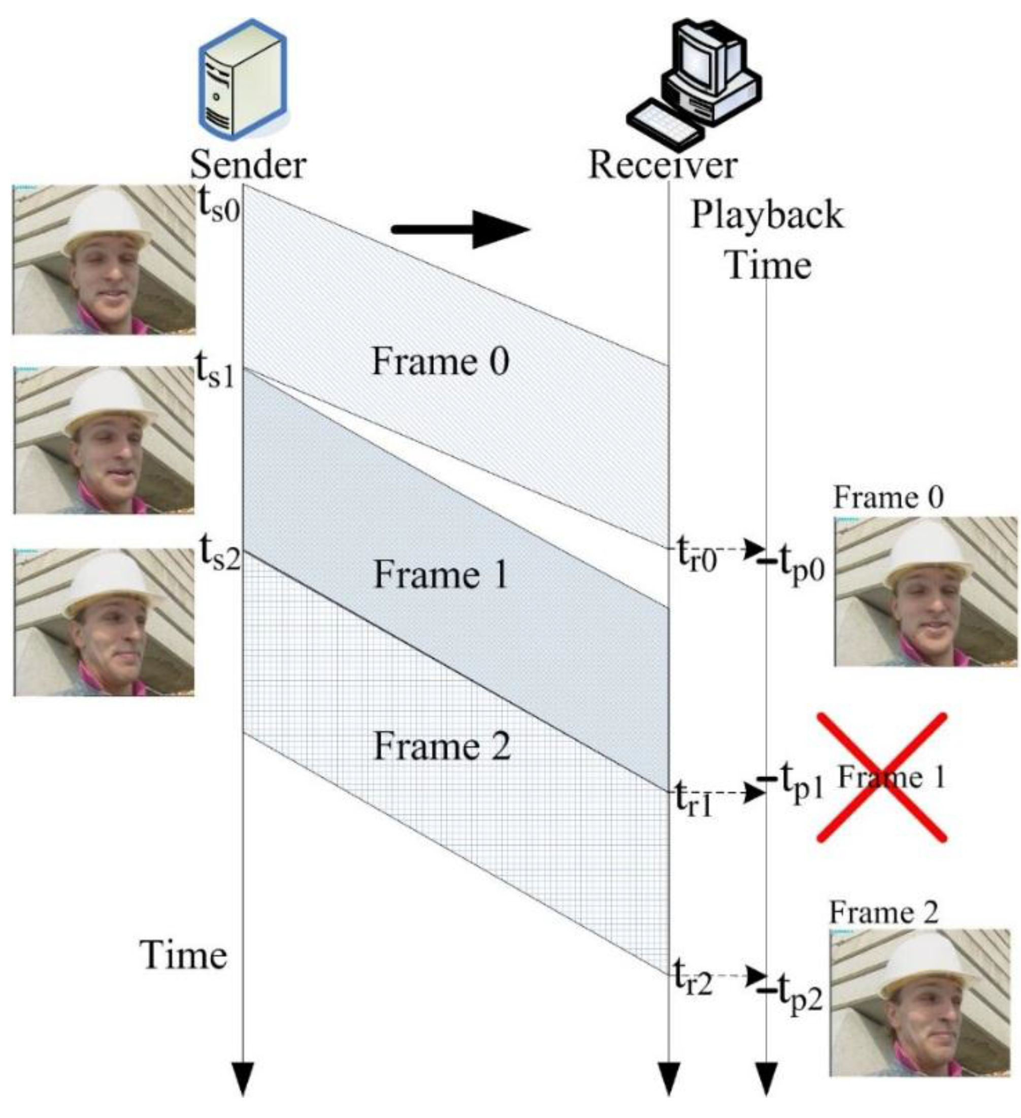
2.1. Effect of Jitter to Perceptual Video Quality

If there are no variations in delay, the time between two consecutive pieces of data will never change; the flow of video observed at the receiver is as smooth as at the sender side. If jitter is present the time between consecutive packets is unknown prior to delivery. In Internet traffic jitter can be of the order of hundreds of milliseconds which has the potential to distort the video [3].

Figure 1 shows the effects jitter can have on continuity. In the figure the frame arriving after its decoding time will never be displayed. Loss concealment can be applied to repair the distortion but at the expense of reduced video quality. The impact of the continuity on perceived video quality has been investigated in [8,9].

As a result of jitter, the perceptual quality is reduced and it has nearly the same effect as packet loss [10].

2.2. Jitter Buffer

The primary mechanism to cope with playback interruption is to create a jitter or playback buffer at the receiver [11,12] where the incoming data are stored temporally before playback. The main problem with using only playback buffer to cope with bandwidth fluctuation is that in the event of high jitter, the end-to-end delay and playback delay will be high as well [13]. This research proposes a different approach, which is able to support each other boosting immunity to jitter.

2.3. Scalable Video and Its Flexibility

Much work has been done on scalable video and its ability to adapt; either to shrink or stretch to suit the available bandwidth and user preferences [14,15]. In addition to being flexible in unstable network conditions, the SVC is also capable of adjusting according to: the quality of the picture, the bit-rate or even the power limitations of the display device [16]. In [17], the collaborative streams share the same bottleneck link in a home network. Bandwidth probing estimates the available transmission bandwidth and the SVC flow is then adjusted to suit the channel capacity. The study in [18] uses two Transmission Control Protocol (TCP) connections to transmit one scalable video session with one TCP connection dedicated to the base layer and one TCP connection for all the other enhancement layers. Using parallel TCP connections gives more tolerance to congestion and jitter, however, the higher tolerance gives protection to the base and enhancements equally. The research in [19] presents an efficient video adaptation scheme in the Long-Term Evolution (LTE) networks using the distance between user equipment and the LTE base station as a metric to reduce the size of the scalable video stream.

Figure 2 illustrates the idea of packet removal in scalable video. Some of the NAL units can be removed from the video stream by the sender, if bandwidth is scarce. Although in the figure the top layer NAL unit is discarded, the frame is still decodable albeit at lower quality. Packet removal is the primary method to adjust bit-rate in the SVC.

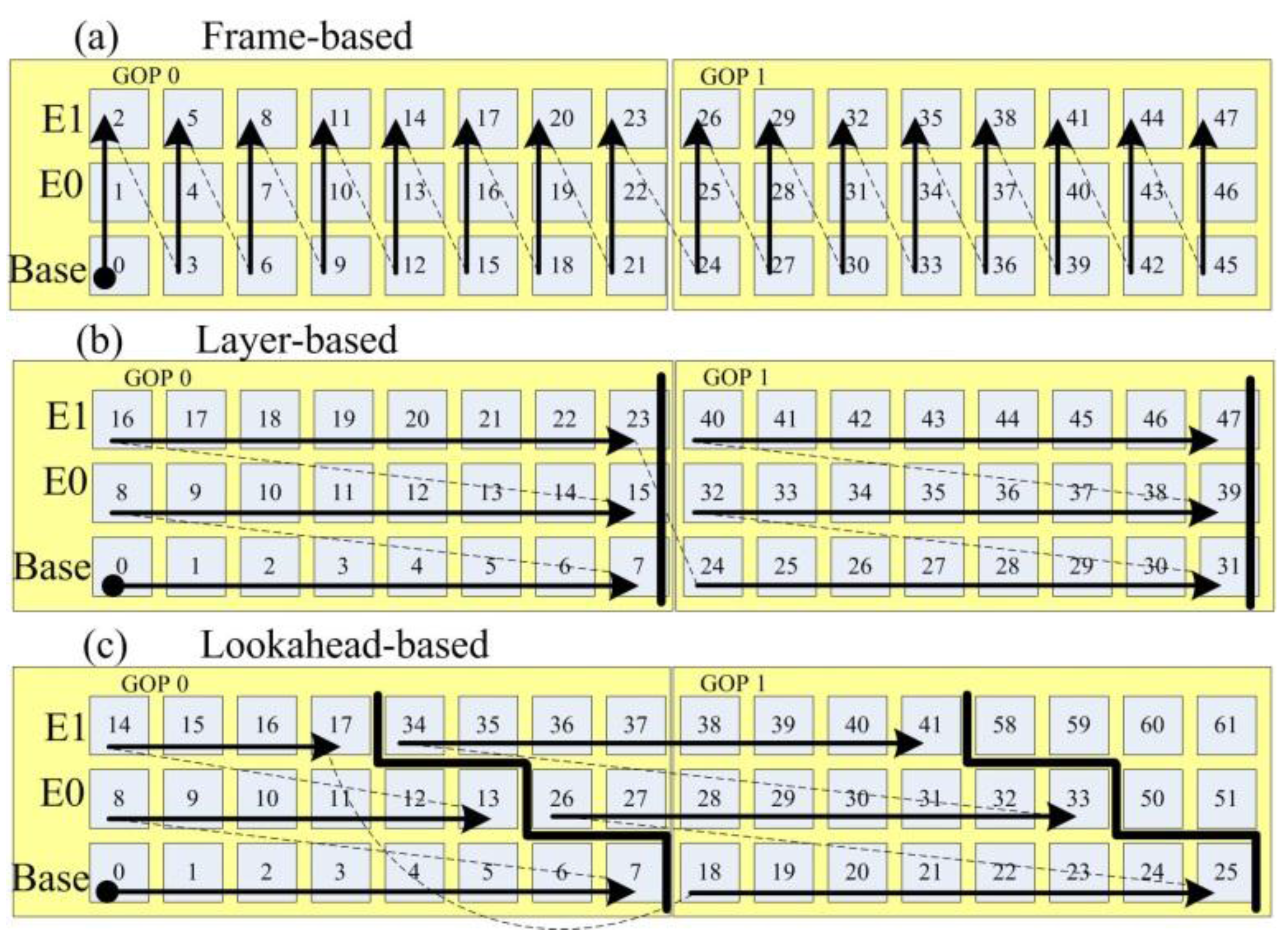
2.4. Scalable Video Scheduling, Reordering and Packet Selection

Layer-based and frame-based scheduling algorithms are mixed to suite the congestion and jitter level [17]. In the case of high congestion the layer-based scheme will produce better results. If the network is stable, frame-based scheduling is best employed. Alternatively packet selection schemes can be employed to reduce bit-rate, where the objective is to adjust the bit-rate by selecting the best group of packets that minimize the distortion [20,21,22]. The 3D scalable video scheduling in P2P networks was proposed in [23]. In this study, a client chooses the appropriate layers of scalable video along with a suitable depth according to the limited download bandwidth. The algorithm in this study also provides checking to guarantee the smoothness of the video by considering the playback deadline of each video packet in the base layer. The technique proposed in [24] is used to transmit scalable video streaming in MC-CDMA. To improve video quality, this study used partial channel state information (PCSI) to give different priorities to each layer of scalable video. The study in [25] proposed a technique using interleaving scheme to prioritize NAL units for real-time MVC video streaming. Other research on packet selection considers the status of the ancestor packets before sending the descendants [26,27]. If an ancestor has not been scheduled, the descendant packet will be discarded. This method reduces the number of the descendant packets that are transmitted but cannot be decoded.

2.5. Unequal Protection

The SVC is a layered video scheme in which the video flow is composed of multiple layers, each with different importance. Unequal error protection can be applied to protect the more important layers using Forward Error Correction (FEC). The research in [28] first applied forward error correction (FEC) to provide prioritization in the network layer rather than more traditional physical layer. FEC is an effective method of protection but adds overhead to the stream. In [5], to increase the quality of video, the researchers give higher priority to the more important layers using Reed-Solomon coding, this is in conjunction with priority-aware block interleaving (PBI) in the MAC layer. The research presented in [29] proposed an unequal recovery algorithm to lost packets which has higher retry transmission rates for the base layer compared to the enhancement layers. However, this algorithm needs a retransmission mechanism to archive the smoothness of video flow.

3. Proposed Algorithm and Its Analysis

We propose a new technique which uses round robin with unequal look ahead scheduling. The Look Ahead Scheduling Algorithm is named as LASA. By setting unequal look-ahead limits to each layer, unequal protection against discontinuity will be achieved. In this algorithm, the base layer is allocated a larger look-ahead limit than the other layers, the probability of a frame with deadline violation is decreased accordingly.

3.1. An Overview of the LASA Scheduling Algorithm

In order to describe LASA scheduling in detail, we compare our algorithm with frame-based and layer-based scheduling. In general, both frame-based and layer-based use traditional round robin scheduling. Frame-based scheduling algorithms schedule all enhancement NAL units which depend on the current base layer NAL unit. In other words, a base layer NAL unit and its enhancement NAL units which represent the same frame will be scheduled consecutively.

In Figure 3, we assume that the scalable video which is composed of a base layer and two enhancement layers has a Group of Pictures (GOP) size of 8. The arrows and numbers show the order of NAL unit scheduling. The notion of a frame-based scheduling algorithm is shown in Figure 3a.

Alternatively, in a layer-based scheduling algorithm, the sending order proceeds along the horizontal axis until the algorithm reaches the upper bound marked by the dark vertical line in Figure 3b, after that the upper layer will be scheduled.

Our LASA scheduling algorithm is shown in Figure 3c. Similar to the layer-based scheduling algorithm, LASA orders the NAL units in the horizontal direction. The unequal bound, which is marked by the dark line, defines the upper bound of NAL units scheduled per layer. In the example shown in Figure 3c, the base layer is allocated with the most look-ahead value, whereas the top layer obtains the least look-ahead value.

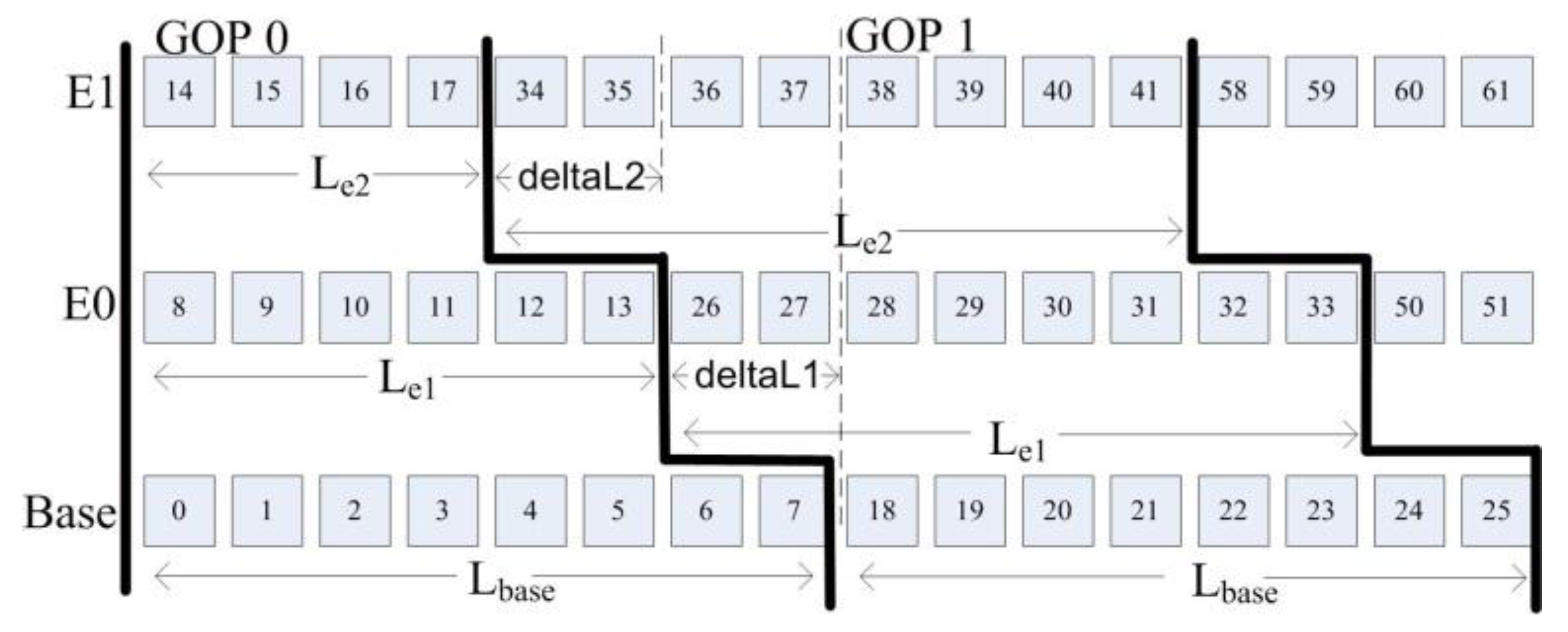
3.2. LASA Scheduling Algorithm and Its Look-Ahead Limit

In this section, we describe the essential parameters of the LASA scheduling algorithm. In Figure 4, there are two type of parameters look-ahead (L_base, L_e1 and L_e2) and deltal_i.

L_base, L_e1 and L_e2 are the look-aheads limit of the base layer, the first enhancement layer and the second enhancement layer, respectively. In the example shown in Figure 4 we assume that the GOP size is 8 and there are 3 layers: base layer, E0, and E1 or layer 0, 1, and 2 respectively. The LASA algorithm starts scheduling at the NAL unit numbered 0 to the NAL unit numbered 7. The value of look-ahead for the base is therefore 8 that is L_base = 7. For layer E0 and E1, L_e1 = 5 and L_e2 = 3 respectively. DeltaL1 is the difference between layer 0 and layer 1 and deltaL2 is the difference between layer 2 and layer 1. Therefore, deltaL_i is the difference between layer i and i−1. The pseudocode of the LASA scheduling algorithm is shown in Algorithm 1.

We can consider that frame based scheduling is when the parameters are assigned to be deltaL = 0, L_base = 1, L_e1 = 1 and L_e2 = 1, respectively and layer-base scheduling is when deltaL = 0, L_base ≥ 1, L_e1 ≥ 1 and L_e2 ≥ 1 respectively. For LASA, the parameters DeltaL > 0, L_base ≥ 1, L_e1 ≥ 1 and L_e2 ≥ 1, respectively.

Algorithm 1. The pseudocode of the LASA scheduling algorithm.

LASA Algorithm: ----------------------------------------------Inintial Section------------------------------------------ - initialize LookAhead of Base layer (0th) to MaxLookAhead - initialize LookAhead of Enhancement layer i (ith) to MaxLookAhead- ${\displaystyle \sum }_{x=1}^{x=i}Delta{L}_x$ , where i is top layer. - initialize current upper bound of layer ith to LookAhead of layer ith - initialize current NAL Unit index of layer ith to 0 --------------------------------------------Main Section---------------------------------------------- While (NOT All Layers Reach End Of Frame Sequence) For each layer i = 0th to Top Layer While (current NAL Unit index of layer ith <= current upper bound of layer ith AND current NAL Unit index of layer ith <= LastFrame ) - send current NAL Unit of layer ith - Increment current NAL unit index of layer ith EndWhile - set current upper bound of layer ith to current upper bound of ith + LookAhead of layer ith - set LookAhead of layer ith to MaxLookAhead EndFor EndWhile

3.3. An Analysis of the LASA Scheduling Algorithm

Mathematical Analysis

This section is dedicated to the analysis of the LASA algorithm in which we show that the sending time for NAL units in the base layer, scheduled by LASA have sending times less or equal to layer-based scheduling.

We define the following terms:

• $t_{la{y}_{[g,l,i]} }^s$ is the time when layer-based scheduling starts sending a NAL unit $g,l,i$ where
• $g$ is a group of pictures number, $g\in I, g\ge 0$
• $l$ is the layer number, $l\in I, 0\le l\le l_{max}$
• $i$ is the sending order of frames, $i \in I, 0\le i\le gs$.
• $t_{l{h}_{[g,l,i]}}^s$ is the time when LASA starts sending the first bit of the NAL unit $g,l,i$
• $t_{[g,l,i]}^p$ is the time spent between the beginning of the first bit and the end of a NAL unit $g,l,i$
• $l_{max}$ is the number of layers, so $l_{max}\ge 0$
• $gs$ is GOP size, so $gs\ge 1$

Figure 5 shows the meaning of $t_{[g,l,i]}^s$ and $t_{[g,l,i]}^p$.

The time to start sending any base layer NAL unit is given in Equation (1).

$${{\displaystyle t}}_{{{\displaystyle lay}}_{[x,0,z]}}^s={\displaystyle \sum _{g=0}^{x-1}{\displaystyle \sum _{l=0}^{{{\displaystyle l}}_{\max }}{\displaystyle \sum _{i=0}^{gs-1}{{\displaystyle t}}_{[g,l,i]}^p}}}+{\displaystyle \sum _{i=0}^{z-1}{{\displaystyle t}}_{[x,0,i]}^p}$$

(1)

where $x,z\in Iandx\ge 1,z\ge 1$.

$${{\displaystyle t}}_{{{\displaystyle lh}}_{[x,0,z]}}^s={{\displaystyle t}}_{{{\displaystyle lay}}_{[x,0,z]}}^s-{{\displaystyle t}}_{skip}^p$$

(2)

where $t_{skip}^p$ is the time spent for some NAL units in layer-based scheduling but is not used by LASA scheduling. $t_{skip}^p$ > 0 when DeltaL1 or DeltaL2 > 0 as shown in Figure 6b,c.

In Figure 6b, the time spent sending the NAL unit numbers 29, 37 and 38 is $t_{skip}^p$ of Equation (2) when DeltaL1 = DeltaL2 = 1. So, if we use LASA, the NAL unit marked by B, which would otherwise be numbered 21, will be sent earlier than scheduled by the layer-based approach, as shown in Equation (3).

$${{\displaystyle t}}_{{{\displaystyle lh}}_B}^s<{{\displaystyle t}}_{{{\displaystyle lay}}_B}^s$$

(3)

where:

• $t_{l{h}_B}^s$ is the time when LASA starts sending NAL unit B.
• $t_{la{y}_B}^s$ is the time when the layer-based scheduling algorithm starts sending NAL unit B.
• $t_{29}^p$$t_{37}^p \text{and} t_{38}^p$ are the times spent for sending NAL units 29, 37 and 38, respectively.

In Figure 6c, the time spent sending the NAL units 26, 27, 34, 35, 36 and 37 is $t_{skip}^p$ when DeltaL1 = DeltaL = 2. Therefore, if the NAL unit marked by C is scheduled by LASA, it will be sent earlier than by layer-based scheduling as shown in Equation (4).

$${{\displaystyle t}}_{{{\displaystyle lh}}_C}^s<{{\displaystyle t}}_{{{\displaystyle lay}}_C}^s$$

(4)

With reference to Equation (5), due to $t_{skip}^p>0$, every NAL unit of the base layer which is scheduled by LASA will be sent earlier than the corresponding layer-based scheduling algorithm.

$${{\displaystyle t}}_{{{\displaystyle lh}}_{[x,0,z]}}^s<{{\displaystyle t}}_{{{\displaystyle lay}}_{[x,0,z]}}^s$$

(5)

In the case of the first GOP where$t_{skip}^p=0$, LASA has not skipped any NAL units. Therefore, in this case, we have

$${{\displaystyle t}}_{{{\displaystyle lh}}_{[x,0,z]}}^s={{\displaystyle t}}_{{{\displaystyle lay}}_{[x,0,z]}}^s$$

(6)

Referring to Equations (5) and (6), we can conclude that the starting time of any base layer NAL unit transmitted by LASA is less than or equal to that of the layer-based scheduling algorithm. The “sooner the better” approach for scheduling the base layer adopted by LASA is the reason the algorithm is able to provide more jitter protection to the base layer. In unpredictable traffic conditions, it is better if base layer NALs have as much time as possible to allow for the unpredictable delay.

Therefore, the result of comparing LASA scheduling and layer scheduling algorithms with respect to sending time is shown in Equation (7).

$${{\displaystyle t}}_{{{\displaystyle lh}}_{[x,0,z]}}^s\le {{\displaystyle t}}_{{{\displaystyle lay}}_{[x,0,z]}}^s$$

(7)

Next, layer-based and frame-based scheduling algorithms are analyzed.

$$\begin{array}{ll}{{\displaystyle t}}_{{{\displaystyle frm}}_{[x,0,z]}}^s=& {\displaystyle \sum _{g=0}^{x-1}{\displaystyle \sum _{i=0}^{gs-1}{\displaystyle \sum _{l=0}^{{{\displaystyle l}}_{\max }}{{\displaystyle t}}_{[g,l,i]}^p}}}+{\displaystyle \sum _{i=0}^{z-1}{{\displaystyle t}}_{[x,0,i]}^p}+\\ & {\displaystyle \sum _{i=0}^{z-1}{{\displaystyle t}}_{[x,1,i]}^p}+{\displaystyle \sum _{i=0}^{z-1}{{\displaystyle t}}_{[x,2,i]}^p}\end{array}$$

(8)

With reference to Equations (1) and (8), note that, the first and the second terms of Equations (1) are (8). Therefore

$${{\displaystyle t}}_{{{\displaystyle frm}}_{[x,0,z]}}^s={{\displaystyle t}}_{{{\displaystyle lay}}_{[x,0,z]}}^s+{\displaystyle \sum _{i=0}^{z-1}{{\displaystyle t}}_{[x,1,i]}^p+{\displaystyle \sum _{i=0}^{z-1}{{\displaystyle t}}_{[x,2,i]}^p}}$$

(9)

Because of ${\displaystyle \sum _{i=0}^{z-1}{{\displaystyle t}}_{[x,1,i]}^p\ge 0}$ and ${\displaystyle \sum _{i=0}^{z-1}{{\displaystyle t}}_{[x,2,i]}^p}\ge 0$, so we obtain

$${{\displaystyle t}}_{{{\displaystyle frm}}_{[x,0,z]}}^s\ge {{\displaystyle t}}_{{{\displaystyle lay}}_{[x,0,z]}}^s$$

(10)

From Equations (7) and (10), we conclude that the base layer NAL unit will receive greater benefit using LASA scheduling than layer-based and frame-based scheduling with respect to the start time of transmission. The order of the starting times for the three different scheduling algorithms is shown in Equation (11).

$${{\displaystyle t}}_{{{\displaystyle lh}}_{[x,0,z]}}^s\le {{\displaystyle t}}_{{{\displaystyle lay}}_{[x,0,z]}}^s\le {{\displaystyle t}}_{{{\displaystyle frm}}_{[x,0,z]}}^s$$

(11)

In the next section, the performance of the LASA scheduling algorithm will be evaluated through simulation.

4. Simulation Results

This section is dedicated to the simulation of the LASA scheduling algorithm. The simulation is conducted in a rapidly fluctuating jitter-prone scenario using the network simulator (NS3).

4.1. Simulation Setup

Figure 7 depicts the dumbbell topology constructed for the simulation. Two pairs of end nodes are connected together and share a bottleneck link. All link capacities are set to 2.2 Mb/s and 20 ms for transmission delay. In order to generate rapidly fluctuating bandwidths, an ON/OFF UDP flow with an exponential random variable has been used for the background traffic. The mean ON time period is varied from 0.0 to 0.4 s. The mean OFF period is 1s and the mean UDP packet is set to 1000 bytes.

We concatenated five public frame sequences which are city, foreman, mobile, soccer and harbor. All video clips are 30 fps, 300 frames and CIF (352 × 288) resolution. This concatenated video is encoded with average bitrate of 1541 kbps by the JSVM reference software [30] and is injected into the NS3 simulator. In the decoding process, the Open SVC Decoder is employed [31,32]. The encoded video is composed of a base layer and two enhancement layers. We use a GOP of 16 frames. In each simulation run, we inject the bit-stream of the concatenated video to the network simulator by setting 60 s of simulation time for each run. We also repeat our simulation with different seeds for the random variable in order to vary the background traffic pattern.

All three scheduling algorithms (LASA, layer-based, and frame-based) were implemented and compared. In the same way as other streaming video research, the buffer has also been added as part of the simulation to collect NAL units. When pre-buffering threshold is reached, the receiver will start decoding and playout [13].

In the playback buffer management module, it also stamps the receiving time of each NAL unit. If some NAL units arrive at the receiver later than their deadlines, those NAL units will be marked as deadline violations which will not be passed to the decoder. We collected the receiving time of each NAL unit to analyze the number of frames that miss their deadlines.

All undecodable frames either the missed deadline frames, lost frames or erroneous frames will be concealed with the previous frame in order to maintain the number of frames in the video sequence. In line with other researchers [33] we compare Y PSNR between the original YUV and distorted YUV as shown in Figure 7.

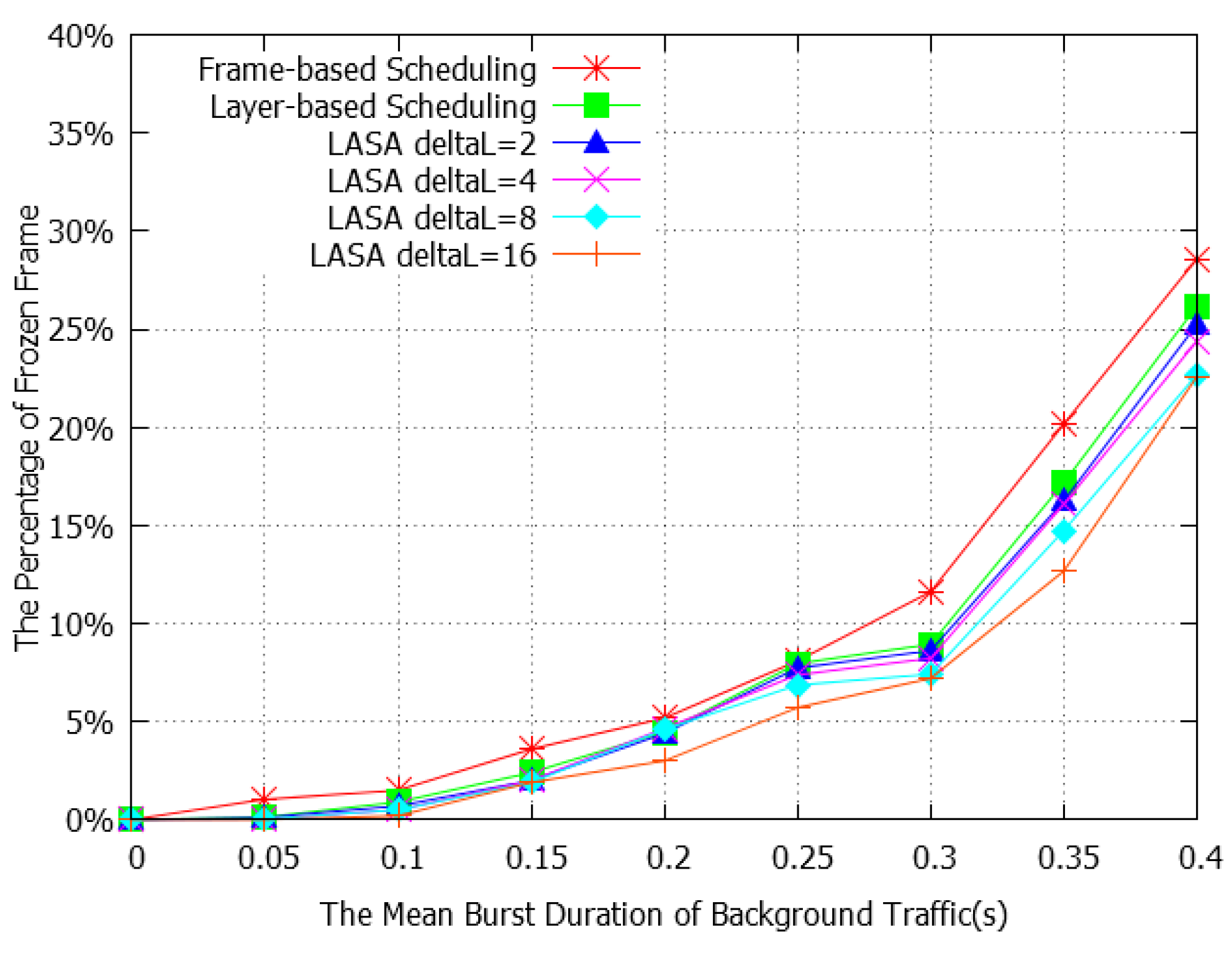
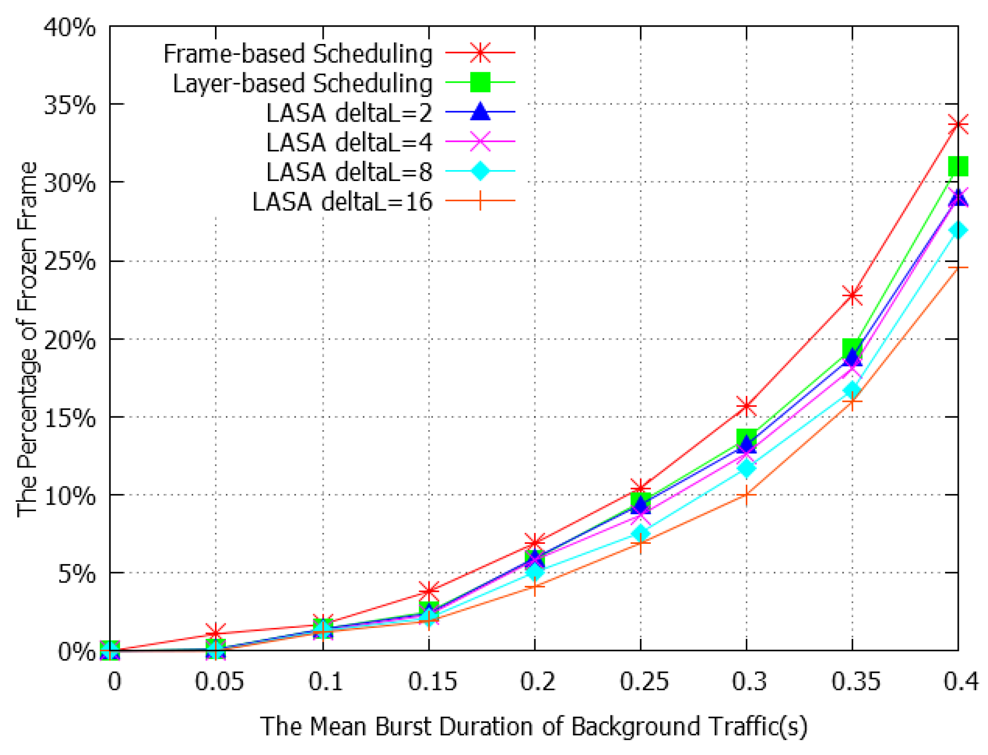
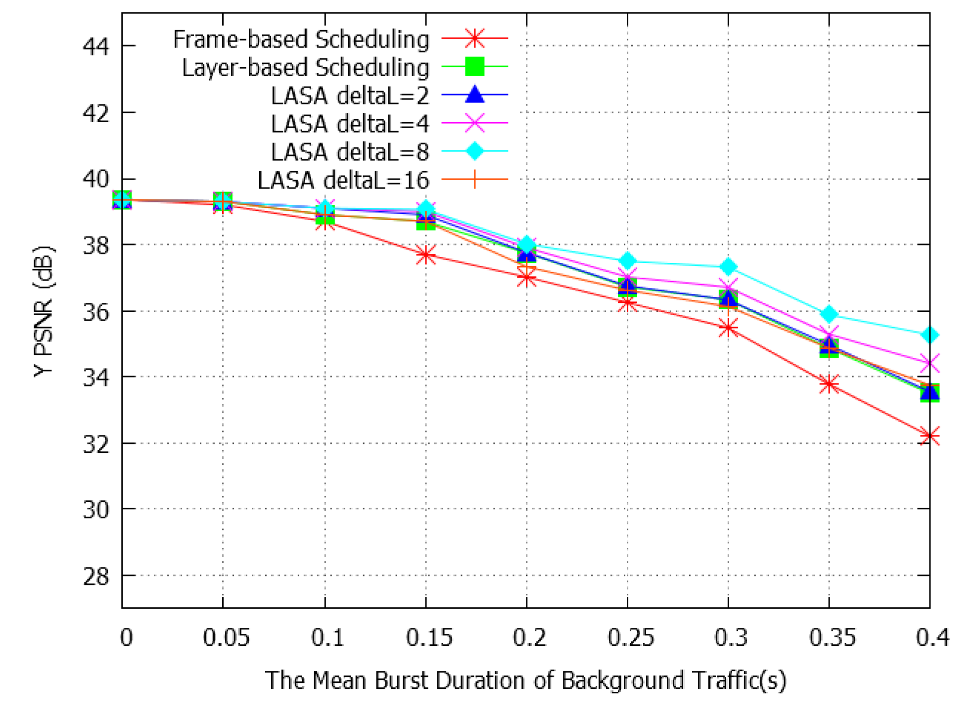
4.2. Performance Evaluation

In this experiment, we compare the performance of the three algorithms by concentrating on the continuity and the average Y PSNR. The result of LASA scheduling reveals that the number of frames that miss the deadline and the number of concealed frames is lower than the layer-based and frame-based scheduling algorithms. LASA scheduling with deltaL equal to 2, 4 or 8 is able to improve results but for deltaL equal to 16 the average Y-PSNR is very similar to layer-based scheduling, but higher than the frame-based method.

The essential parameters are varied. Firstly, the ON time period of background traffic is varied between 0.0 to 0.4 s to produce jitter. Secondly, we vary the pre-buffering threshold of the playback buffer. The larger is the playback buffer the better it is in terms of its ability to resist jitter. We, therefore, vary the period of time before beginning playback from 400 to 600 ms.

In Figure 8, Figure 9 and Figure 10, the percentages of missed deadlines among the three algorithms are observed.

In Figure 8, the playback buffer threshold is set to 600 ms, the percentage of missed deadline frames for LASA scheduling is lower than layer-based scheduling. LASA scheduling is able to reduce the number of frames missing the deadline considerably. For the case of LASA with deltaL equal to 16, when high burst duration (0.2 to 0.4) is injected, the percentage of missed deadline frames is 0.84% lower than layer-based scheduling on average.

To increase the influence of jitter we reduced the play out buffer from 600 to 500 ms and 400 ms as shown in Figure 9 and Figure 10. As summarized in

Table 1. Comparison of the percentage of missed deadline frames between layer-based and the LASA scheduling algorithm when burst duration is varied from 0.2 to 0.4 s.

Threshold	deltaL = 2	deltaL = 4	deltaL = 8	deltaL = 16
400 ms	−0.03	−0.42	−0.88	−1.43
500 ms	−0.01	−0.32	−0.64	−1.11
600 ms	−0.18	−0.29	−0.54	−0.84
Average	−0.07	−0.34	−0.69	−1.13

, the largest improvement provided by LASA is when deltaL = 16; around 1.43%. When deltaL are 2, 4 or 8, the percentage of missed deadlines are still lower than the layer-based approach. The negative values seen in Table 1 are representative of when LASA is providing improved results over layer-based scheduling.

LASA scheduling has the highest performance of the three scheduling algorithms with respect to the number of frames that have arrived at the receiver after the deadline for playback. The results for buffer thresholds of 600, 500, and 400 ms as shown in Figure 8, Figure 9 and Figure 10, respectively. These results agree with the mathematical analysis in Equation (11) and our assumption that if we send important NAL units earlier, there is more time to overcome unpredictable delays, and the probability of missing the deadline will be reduced accordingly.

As some base layer NAL units may miss their decoding deadline, or being lost or are in errors, they cause some descendant NAL units not to be decoded even if they arrive at the receiver before the deadline. All undecodable frames will be concealed with their previous frames. The percentages of the undecodable frames are shown in Figure 11, Figure 12 and Figure 13. From the user’s perspective, if the number of frozen frames increases, the continuity of the video stream decreases.

In Figure 11, the percentage of frozen frames for LASA scheduling is lower than layer-based and frame-based scheduling. For example, on high burst duration (0.2–0.4 s) LASA with deltaL = 16 is lower than layer-based scheduling by 2.71%. For thresholds of 500 ms, and 400 ms as shown in Figure 12 and Figure 13, the percentages of frozen frames for LASA are lower than layer-based by 3.56% and 4.60% respectively. In

Table 2. Comparison of the percentage of frozen frames between layer-based and the LASA scheduling algorithm when burst duration is varied from 0.2 to 0.4 s.

Threshold	deltaL = 2	deltaL = 4	deltaL = 8	deltaL = 16
400 ms	0.18	−1.14	−2.81	−4.60
500 ms	−0.59	−1.01	−2.27	−3.56
600 ms	−0.50	−0.80	−1.69	−2.71
Average	−0.30	−0.98	−2.25	−3.63

, we compare the percentage of frozen frames between layer-based and LASA. The negative value corresponds to when LASA is better than layer-based in terms of frozen frames.

LASA scheduling is designed to give more protection to the base layer by sacrificing enhancement layer protection. However, since the loss of base layer data is more damaging than the loss of enhancement data, the overall video quality may not be degraded that much. Moreover, in the LASA algorithm even if we lose video quality in some frames but we gain video continuity by reducing the percentage of frozen frames compared to other rival algorithms. Hence the overall video quality is improved.

Figure 14, Figure 15 and Figure 16 show that LASA scheduling with deltaL equal to 8 either for 400 ms, 500 ms or 600 ms thresholds is able to improve the Y PSNR significantly by 0.92 dB, 0.96 dB and 0.69 dB, respectively. For LASA scheduling with deltaL equals to 4, Y PSNR is improved by 0.44 dB, 0.43 dB and 0.37 dB. However, in the case of deltaL = 2 and deltaL = 16 the average Y PSNR is similar to layer-based scheduling. In

Table 3. Comparison of Average Y PSNR, in dB, between Layer-based and LASA scheduling algorithms when burst duration is varied from 0.2 to 0.4 s.

Threshold	deltaL = 2	deltaL = 4	deltaL = 8	deltaL = 16
400 ms	0.04	0.44	0.92	−0.09
500 ms	0.04	0.43	0.96	−0.09
600 ms	0.06	0.37	0.69	−0.09
Average	0.05	0.41	0.86	−0.09

, we summarize the average Y PSNR of LASA and layer-based scheduling. It should be noticed that, both LASA and layer-based scheduling are better than frame-based.

In Table 3, negative values represent when LASA has a lower PSNR than layer-based scheduling whilst a positive value represents higher. The difference of the average Y PSNR of LASA and layer-based scheduling vary between -0.09 dB to 0.96 dB and it is only when deltaL is equal to 16 that a negative value is obtained.

Due to the parameter deltaL of LASA, sending enhancement layer NAL units can incur delays. To enable the receiver to play the video at the highest quality layer, the per-buffering time setting should exceed the time value $t$ in (12).

$${{\displaystyle t}}_{}=\frac{{\displaystyle \sum _{i=0}^{Top-1}(deltaL*(Top-i))(\frac{B{r}_i}{F{r}_i})}}{AverageBandwidth}$$

(12)

where t is pre-buffering time, $B{r}_i$ is average bitrate of layer i, $F{r}_i$ is frame rate of layer i and Top is the top available layer.

5. Conclusions and Discussion

The main contribution of the LASA scheduling algorithm, presented in this paper, is improved continuity of a video stream in a jitter-prone environment by providing an unequal look-ahead value to each layer of a scalable video. It is able to maintain or improve the average Y PSNR compared to layer-based and frame-based scheduling algorithms. In addition to the PSNR improvement of LASA by up to 4 dB, the continuity of the video is also improved. This quality measurement can be more significant subjectively, as at high video qualities, 4 dB improvement may not be appreciated, but continuity is notable.

By exploiting the flexibility of the scalable video architecture in which a video is composed of one or more layers of unequal importance, improvements in dropped frames and PSNR are demonstrated. With predefined unequal look-ahead values, the base layer scheduled by LASA provides improved safety to the base layer and means the enhancement NAL units do not get discarded.

In addition, the novel approach for jitter resistance of LASA can be integrated with standard playback buffers to improve performance further, if higher end-to-end delay is permissible.

References

1. ITU-T. Analysis, Measurement and Modelling of Jitter. In ITU-T Delayed Contribution COM 12—D98; ITU-T: Geneva, Switzerland, 2003. [Google Scholar]
2. Bertsekas, D.; Gallager, R. Data Networks, 2nd ed.; Prentice-Hall, Inc.: Upper Saddle River, NJ, USA, 1992; p. 556. [Google Scholar]
3. Venkataraman, M.; Chatterjee, M. Quantifying video-qoe degradations of internet links. IEEE/ACM Trans. Netw. 2012, 20, 396–407. [Google Scholar] [CrossRef]
4. ITU-T. Perceptual Video Quality Measurement Techniques for Digital Cable Television in the Presence of a Reduced Reference. In Recommendation ITU-T J.249; ITU-T: Geneva, Switzerland, 2010. [Google Scholar]
5. Kyungtae, K.; Jeon, W.J. Differentiated protection of video layers to improve perceived quality. IEEE Trans. Mob. Computing 2012, 11, 292–304. [Google Scholar] [CrossRef]
6. Schwarz, H.; Marpe, D.; Wiegand, T. Overview of the scalable video coding extension of the h.264/avc standard. IEEE Trans. Circuits Syst. Video Technol. 2007, 17, 1103–1120. [Google Scholar] [CrossRef]
7. Palawan, A.; Woods, J.; Ghanbari, M. A jitter-tolerant scheduling algorithm to improve continuity in scalable video streaming. In Proceedings of the 2015 7th Computer Science and Electronic Engineering Conference (CEEC), Colchester, UK, 24–25 September 2015.
8. Huynh-Thu, Q.; Ghanbari, M. Impact of jitter and jerkiness on perceived video quality. In Proceedings of the Workshop on Video Processing and Quality Metrics, Scottsdale, AZ, USA, 1–4 January 2006.
9. Huynh-Thu, Q.; Ghanbari, M. Temporal aspect of perceived quality in mobile video broadcasting. IEEE Trans. Broadcast. 2008, 54, 641–651. [Google Scholar] [CrossRef]
10. Claypool, M.; Tanner, J. The effects of jitter on the peceptual quality of video. In Proceedings of the seventh ACM international conference on Multimedia (Part 2), Orlando, FL, USA, 30 October 1999; pp. 115–118.
11. Su, Y.-F.; Yang, Y.-H.; Lu, M.-T.; Chen, H.H. Smooth control of adaptive media playout for video streaming. Trans. Multi. 2009, 11, 1331–1339. [Google Scholar]
12. Kalman, M.; Steinbach, E.; Girod, B. Adaptive media playout for low-delay video streaming over error-prone channels. IEEE Trans. Circuits Syst. Video Technol. 2004, 14, 841–851. [Google Scholar] [CrossRef]
13. Liang, G.; Liang, B. Balancing interruption frequency and buffering penalties in vbr video streaming. In Proceedigns of the 2007 26th IEEE International Conference on Computer Communications, IEEE INFOCOM, Anchorage, AK, USA, 6–12 May 2007; pp. 1406–1414.
14. Choi, H.; Kang, J.; Kim, J.-G. Dynamic and interoperable adaptation of SVC for QoS-enabled streaming. IEEE Trans. Consum. Electron. 2007, 53, 384–389. [Google Scholar] [CrossRef]
15. Wien, M.; Cazoulat, R.; Graffunder, A.; Hutter, A.; Amon, P. Real-time system for adaptive video streaming based on SVC. IEEE Trans. Circuits Syst. Video Technol. 2007, 17, 1227–1237. [Google Scholar] [CrossRef]
16. Lee, H.; Lee, Y.; Lee, J.; Lee, D.; Shin, H. Design of a mobile video streaming system using adaptive spatial resolution control. IEEE Trans. Consum. Electron. 2009, 55, 1682–1689. [Google Scholar] [CrossRef]
17. Kim, D.; Chung, K. A network-aware quality adaptation scheme for device collaboration service in home networks. IEEE Trans. Consum. Electron. 2012, 58, 374–381. [Google Scholar] [CrossRef]
18. Chaurasia, A.K.; Jagannatham, A.K. Dynamic parallel tcp for scalable video streaming over mimo wireless networks. In Procedings of the 2013 6th Joint IFIP, Wireless and Mobile Networking Conference (WMNC), Dubai, United Arab Emirates, 23–25 April 2013; pp. 1–6.
19. Radhakrishnan, R.; Nayak, A. An efficient video adaptation scheme for svc transport over lte networks. In Proceedings of the 2011 IEEE 17th International Conference on Parallel and Distributed Systems (ICPADS), Tainan, Taiwan, 7–9 December 2011; pp. 127–133.
20. Maani, E.; Yijing, L.; Pahalawatta, P.; Katsaggelos, A. Packet scheduling for scalable video streaming over lossy packet access networks. In Proceedings of 16th International Conference on Computer Communications and Networks, 2007, ICCCN 2007, Honolulu, HI, USA, 13–16 August 2007; pp. 591–596.
21. Miao, Z.; Ortega, A. Optimal scheduling for streaming of scalable media. In Proceedigns of the 2000 Conference Record of the Thirty-Fourth Asilomar Conference on Signals, Systems and Computers, Pacific Grove, CA, USA, 29 October–1 November 2000; Volume 1352, pp. 1357–1362.
22. Chou, P.A.; Zhourong, M. Rate-distortion optimized streaming of packetized media. IEEE Trans. Multimedia 2006, 8, 390–404. [Google Scholar] [CrossRef]
23. Liu, Y.; Liu, J.; Song, J.; Argyriou, A. Scalable 3d video streaming over p2p networks with playback length changeable chunk segmentation. J. Visual Commun. Image Represent. 2015, 31, 41–53. [Google Scholar] [CrossRef]
24. Seo, H.; Lee, K. Effective scalable video streaming transmission with TBS algorithm in an MC-CDMA system. Inf. Syst. 2015, 48, 313–319. [Google Scholar] [CrossRef]
25. Liu, Z.; Qiao, Y.; Karunakar, A.K.; Lee, B.; Fallon, E.; Zhang, C.; Zhang, S. H. 264/mvc interleaving for real-time multiview video streaming. J. Real-Time Image Process. 2015, 10, 501–511. [Google Scholar] [CrossRef]
26. Jurca, D.; Frossard, P. Video packet selection and scheduling for multipath streaming. IEEE Trans. Multimedia 2007, 9, 629–641. [Google Scholar] [CrossRef]
27. De Vleeschouwer, C.; Frossard, P. Dependent packet transmission policies in rate-distortion optimized media scheduling. IEEE Trans. Multimedia 2007, 9, 1241–1258. [Google Scholar] [CrossRef]
28. Hellge, C.; Gomez-Barquero, D.; Schierl, T.; Wiegand, T. Layer-aware forward error correction for mobile broadcast of layered media. IEEE Trans. Multimedia 2011, 13, 551–562. [Google Scholar] [CrossRef]
29. Kuo, W.H.; Kaliski, R.; Wei, H.Y. A qoe-based link adaptation scheme for H.264/SVC video multicast over IEEE 802.11. IEEE Trans. Circuits Syst. Video Technol. 2015, 25, 812–826. [Google Scholar] [CrossRef]
30. JVT. Iso/iec 14496–10 amd.3 Scalable Video Coding. In Doc. JVT-X201; ITU-T: Geneva, Switzerland, 2007. [Google Scholar]
31. Blestel, M.; Raulet, M. Open SVC decoder: A flexible SVC library. In Proceedings of the international conference on Multimedia, Firenze, Italy, 8–10 October 2010; pp. 1463–1466.
32. Pescador, F.; Samper, D.; Raulet, M.; Juarez, E.; Sanz, C. A DSP based H.264/SVC decoder for a multimedia terminal. In Proceedigns of the 2011 IEEE International Conference on Consumer Electronics (ICCE), Las Vegas, NV, USA, 9–12 January 2011; pp. 401–402.
33. Cho, Y.; Kwon, D.K.; Liu, J.; Kuo, C.J. Dependent r/d modeling techniques and joint t-q layer bit allocation for H.264/SVC. IEEE Trans. Circuits Syst. Video Technol. 2013, 23, 1003–1015. [Google Scholar] [CrossRef]
Figure 1. Jitter or variation of delay causes degradation in continuity of a video stream.
Computers 05 00011 g001
Figure 2. An example of possible Network Abstraction Layer (NAL) unit removal in scalable video.
Computers 05 00011 g002
Figure 3. The concept of the three different scheduling schemes discussed. (a) A frame-based scheduling algorithm; (b) A layer-based scheduling algorithm; and (c) The Look Ahead Scheduling Algorithm (LASA) scheduling algorithm.
Computers 05 00011 g003
Figure 4. Look-ahead value is allocated to each layer unequally.
Computers 05 00011 g004
Figure 5. Definition of the time to start sending ( t [ g , l , i ] s ) and time spent for sending each NAL unit ( t [ g , l , i ] p ) used in this section.
Computers 05 00011 g005
Figure 6. The values of t s k i p p when (a) DeltaL1 = DeltaL2 = 0 and t s k i p p = 0 ; (b) DeltaL1 = DeltaL2 = 1 and   t s k i p p =   t 29 p +   t 37 p +   t 38 p ; (c) DeltaL1 = DeltaL2 = 2 and t s k i p p =   t 26 p +   t 27 p +   t 34 p   +   t 35 p +   t 36 p +   t 37 p .
Computers 05 00011 g006
Figure 7. Network topology and input/output video stream used in this simulation.
Computers 05 00011 g007
Figure 8. The number of frames with deadline violation when the threshold is 600 ms.
Computers 05 00011 g008
Figure 9. The number of frames with deadline violation when the threshold is 500 ms.
Computers 05 00011 g009
Figure 10. The number of frames with deadline violation when the threshold is 400 ms.
Computers 05 00011 g010
Figure 11. The number of frozen frames when threshold is 600 ms.
Computers 05 00011 g011
Figure 12. The number of frozen frames when threshold is 500 ms.
Computers 05 00011 g012
Figure 13. The number of frozen frames when threshold is 400 ms.
Computers 05 00011 g013
Figure 14. The average Y Peek Signal-to-Noise Ratio (PSNR) when the threshold of the playback buffer is 400 ms.
Computers 05 00011 g014
Figure 15. The average Y PSNR when the threshold of the playback buffer is 500 ms.
Computers 05 00011 g015
Figure 16. The average Y PSNR when the threshold of the playback buffer is 600 ms.
Computers 05 00011 g016