Discrete Event Simulation Method as a Tool for Improvement of Manufacturing Systems

Abstract

The problem of production flow in manufacturing systems is analyzed. The machines can be operated by workers or by robots, since breakdowns and human factors destabilize the production processes that robots are preferred to perform. The problem is how to determine the real difference in work efficiency between humans and robots. We present an analysis of the production efficiency and reliability of the press shop lines operated by human operators or industrial robots. This is a problem from the field of Operations Research for which the Discrete Event Simulation (DES) method has been used. Three models have been developed, including the manufacturing line before and after robotization, taking into account stochastic parameters of availability and reliability of the machines, operators, and robots. We apply the OEE (Overall Equipment Effectiveness) indicator to present how the availability, reliability, and quality parameters influence the performance of the workstations, especially in the short run and in the long run. In addition, the stability of the simulation model was analyzed. This approach enables a better representation of real manufacturing processes.

1. Introduction

This paper expands on the conference paper [1] published in the Position Papers of the Federated Conference on Computer Science and Information Systems (FedCSIS-2016).

The industrial revolution caused the replacement of human labor by machinery. However, workers were still needed to handle and control the machines. Currently, we see increasing use of automation and robotization, which replaces human labor. In fact, many industrial robots are used these days, especially for repetitive and high precision tasks (e.g., welding) or activities of monotonous and demanding physical exertion. Industrial robots have mobility similar to that of the human arm, and can perform various complex actions similarly to a human. In addition, they do not get tired and bored. It is estimated that, thanks to robotization, many companies have obtained a reduction in production costs of 50%, an increase in productivity of 30%, and an increase in utilization of more than 85% [2].

The introduction of robotization incurs high costs; therefore, robotization will be profitable only in certain circumstances, including situations with a high level of production, repetitive work and precision tasks, all the while ensuring health and safety at work. Such conditions occur in the automotive industry and that is where most robots are used.

Manufacturing systems can be very complex and difficult to analyze. Therefore, the Discrete Event Simulation (DES) method [3] is widely used for the design of manufacturing systems [4], solving scheduling problems [5], for efficiency [6] and stability analysis [7] of production systems and the design of transportation systems with Automated Guided Vehicles (AGVs) [8].

These are problems that are related to Operational Research that also involves the conceptual design of the systems, the generation of computer models for different scenarios, production planning and control, bottleneck detection, simulation parameter selection (deterministic or stochastic), the impact of different parameters on results (control factors and noise factors), computational complexity, NP-completeness of certain problems, congestion, deadlock and delay in the system, design of experiments, and the statistical analysis of results [9,10,11,12,13].

There are many methods, including mathematical (linear, constraints, stochastic) programming, combinatorial optimization, Petri nets, and scenario analysis, that can be used for modelling and solving the above-mentioned problems, but computer simulation, especially DES, is the most universal. Some of these methods can be implemented into DES; for example, heuristic rules or Petri nets [14,15].

The main advantage of DES is the ability to conduct experiments that cannot be performed on real manufacturing systems, and designing a simulation model helps in gaining knowledge that could lead to the improvement of the real system [16]. Since so much randomness is associated with simulation (random inputs), it can be hard to distinguish whether an observation is a result of system interrelationships or of randomness.

There are many DES software tools dedicated to production process simulation, including ARENA, Enterprise Dynamics, FlexSim, Plant Simulation and others [17,18,19,20].

The design of complex Manufacturing Systems or Flexible Manufacturing Systems (FMS) requires the integration of various aspects, including manufacturing strategies, system architecture, capacity planning, performance evaluation, management techniques, risk appraisal and scenario analysis [21]. The first step of the design process is Conceptual Modelling, which involves moving from a problem situation, through model requirements, to a definition of what is going to be modelled and how [9]. The FMS design activity must respect a set of constraints defining the manufacturing processes, the product requirements, and the design goals. There are some methods and techniques for designing FMS described by [22,23]. The formalism of FMS can be described with the IDEF (Integration DEFinition) family of modeling languages, and is built on the functional modeling language Structured Analysis and Design Technique (SADT), CIMOSA (CIM Open Systems Architecture), GRAI/GIM (Graphs with Results and Activities Interrelated - GRAI Integrated Methodology), GERAM—(Generalized Enterprise Reference Architecture and Methodology), and Object Flow Diagram [24,25,26,27].

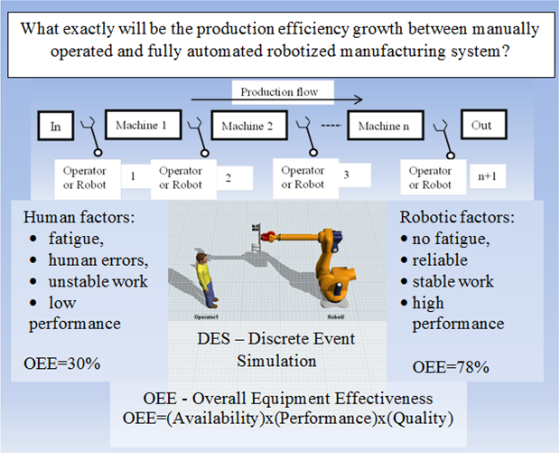
The main problem is how to establish a real difference in the work efficiency between improved or reengineered manufacturing systems, for example, ones that are manually operated and fully automated.

The aim of the current study is to develop a methodology that allows us to clearly define the production efficiency growth associated with an improvement of manufacturing systems, for example, the replacement of human operators with industrial robots. Moreover, the next question is which parameters are important for the evaluation of this problem. That question involves factors related to human–machine interaction. There are many human factors that are difficult to model because of human individuality. In addition, factors related to machine parameters, machine tending, machine and robot reliability and failures, the transportation system, storage system, and quality control system, should all be taken into account.

2. Manufacturing System

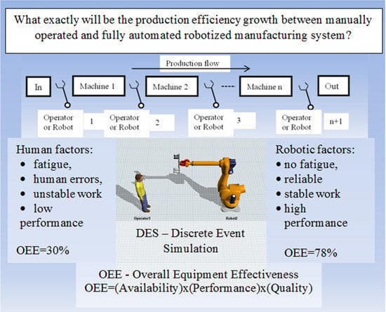
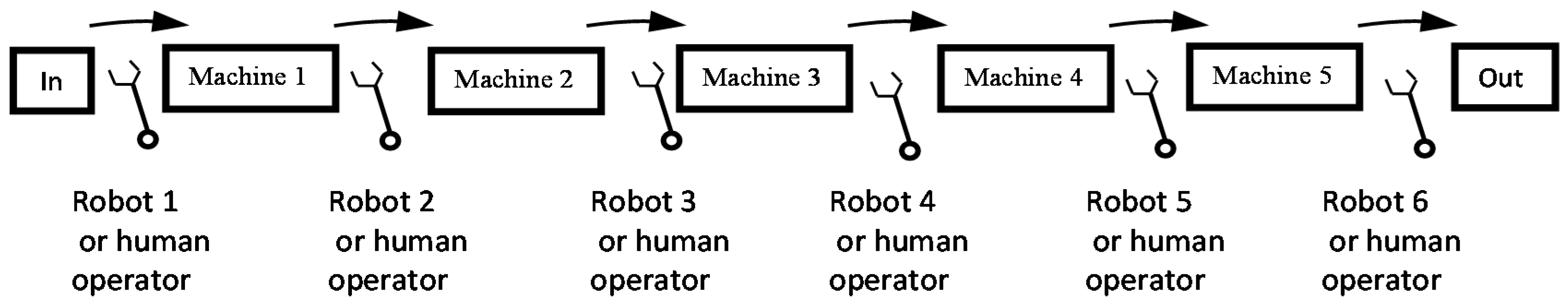
Manufacturing systems consist of different numbers of specialized machines and human operators or robots for material handling. Workstations can be organized as cells or lines. In industry, there are many different types of machine tools, and presses are commonly used. The schema of a typical press line is presented in Figure 1. Usually, an operator is required for loading and unloading the machine and for transferring the product from one machine to the next production stage. Robots can undertake the same work faster and more consistently than human operators, but how fast can a robot work?

Robotized and automated lines typically work very well, but some problems with failures can occur. A failure in any of the elements of the line causes production stoppage of the manufacturing line. Therefore, the reliability of the components plays a key role for the productivity and utilization of the manufacturing system as a whole. Consequently, in practice, the production lines often consist of between four and six machines.

2.1. Availability and Reliability of Machines

The term availability pertains to planned work time and unplanned events, e.g., disturbances at work and random machine failures. Certain unplanned events cause machines to become unavailable, decreasing work efficiency. The reliability of objects, such as machines or robots, is defined as the probability that they will work correctly for a given time under defined conditions of work. The most popular method for estimating reliability parameters uses the theory of probability to forecast a value of any failure-free time and repair time parameters, under the condition that a trend based on historical observations is possible to notice. Examples using normal, exponential, triangular distributions to describe both failure and repair times are described in [28]. In the article [29], it is assumed that the parameters of distributions describing failure-free times, in general, change with time. Based on information about the number of failures and failure-free times in different periods of the same duration in the past, some methods for estimating unknown parameters for scheduling purposes can be proposed [30].

In practice, for the purposes of describing machine reliability, in most cases, the parameter MTTF (mean time to failure) is used, which is the expected value of the time to failure of a machine or system component. For example, if that time is an exponentially distributed random variable with failure rate λ [31], we have:

$$\mathrm{MTTF}={{\displaystyle \int }}_0^{\infty }t\mathrm{f}\left(t\right)\mathrm{d}t={{\displaystyle \int }}_0^{\infty }t\lambda {\mathrm{e}}^{-\lambda t}\mathrm{d}t=\frac{1}{\lambda }$$

(1)

In the case of repairable objects, the parameters MTBF (mean time between failures), and the MTTR (mean time to repair) are used:

$$\mathrm{MTBF}=\mathrm{MTTF}+\mathrm{MTTR}$$

(2)

For complex systems, consisting of n serially linked objects, each of which has exponential failure times with rates λ_i, i = 1, 2, …, n, the resultant overall failure rate λ_S of the system is the sum of the failure rates of each element λ_i:

$${\lambda }_s = {\displaystyle \sum }_{i=1}^n{\lambda }_i$$

(3)

Moreover, the system MTBF_S is the sum of inverse MTBF_i, of linked objects:

$$\frac{1}{{\mathrm{MTBF}}_S}= {\displaystyle \sum }_{i=1}^n\frac{1}{{\mathrm{MTBF}}_i}$$

(4)

For the example of the robotic line presented in Figure 1, we can use Formula (4) with different failure parameters for machines ${\mathrm{MTBF}}_{\mathrm{mi}}$ and ${\mathrm{MTBF}}_{\mathrm{ri}}$ for robots.

2.2. Human Related Factors in Manufacturing

Due to a large variety of production processes, many human factors are studied from different points of view in the areas of engineering, biomechanics, physiology, statistics, psychology and philosophy.

Initial researches in the field were conducted by F. W. Taylor, who began a systematic observation of human workers. His theory was a starting point for modern production engineering and management. It assumes a maximal intensification of works, an efficient usage of operating time and an elimination of the time that is waste. An improvement of the economic efficiency, especially labour productivity, was the main aim of this theory.

Based on many researches presented in the elaboration [32], it was proven that people have an innate predisposition to different kinds of works, e.g., handwork. Young people are more physically fit and efficient than older people (so-called age effect). On the other hand, older people are characterized by greater professional experience, which allows them to work better and more efficiently (experience effect). In addition, psychophysical factors, such as tiredness, illness, and mood swings, have an impact on the performed work.

On the other hand, researches on ergonomics are focused on adapting working conditions to the human abilities. The workplace should be designed taking into account the recommendations of ergonomics (e.g., body position, light, temperature, ventilation, noise) to make labour easier.

Regarding the production flow process, people are characterized by a high variability of behaviours, e.g., when tired, they work with lower efficiency. Moreover, people can cause disturbances in the production process (human errors). Also, accidents at work may be the result of human errors or equipment failures. These accidents may cause an inability to perform future works in production processes.

Since people are very different, there is no universal method for describing the interaction between an operator and a machine. Most often, methods based on mathematical statistics, e.g., MTM (Methods Time Measurement), are used to determine working time standards [33].

Also, in computer software intended for production process simulation, human factors are not sufficiently utilized. When building a computer model, people are treated as a quasi-technical element of the production system and they should operate in the same way as a machine. In practice, human behaviour is unpredictable, which might help to explain why simulation models do not respond to the reality as it would be expected [34].

Knowing the categories of human errors can help to simulate human behaviour more realistically. The planned working time of a human operator can be represented by using a schedule, including the planned interruption of work, such as: preparation of the workstation, setup, testing of machines, cleaning after work completion and meal breaks and rest pause. Planned vacations and excused absences can be omitted because replacements can be arranged [35].

We can also take into account unplanned interruptions at work: short-term interruption resulting from a variety of psycho–physical conditions, for example, physiological needs and long-term interruptions associated with sudden disease or accident at work.

We can model them as machine failures and describe them using exponential distribution with a constant failure rate. Considering the average length of human absence because of health problems is 2 × 5 days per year with 250 working days per year [36], the probability of an employee absence can be described using the parameters MTBF = 125 days and MTTR = 40 h. In turn, short breaks are difficult to estimate because of human individuality and can be approximated using the parameters MTBF = 4–8 h and MTTR = 5–10 min.

For example, assuming human unreliability on the basis of HEART (Human Error Assessment and Reduction Technique) for “routine and highly practiced rapid tasks involving a relatively low level of skill”, the nominal value of human error equals to 0.01 [37]. Therefore, the human error rate can be described by parameters: MTBFh = 8 h and MTTRh = 5 min.

2.3. Robotic Factors in Manufacturing

Modern industrial robots are characterized by a high precision of operation, high speed of motion and high reliability of work. They can be equipped with various tools and used for different works that are traditionally performed by human workers. It is important that robots can work in conditions that are harmful to human health.

Some new-generation robots are equipped with various intelligent sensors, e.g., vision and pattern recognition systems, and they are able to adapt to changing conditions of external surroundings. New generation of robots also have greater speed than older ones and can have an important effect on the robotic system performance.

Theoretically, robots can work 24 h per day without any breaks, but human supervision of the production process as well as precise planning and scheduling of robot work are necessary for better performance [5]. Changes of tools and reprogramming, which are conducted from time to time, require the participation of an operator. Moreover, a robot requires periodic maintenance service and inspection before each automatic run.

There are some methods for robot motion planning described in [38,39]. These methods are based on the MTM or on the traditional time study concept and can be used for comparing the relative abilities of robots and humans. Dedicated computer software for robot movement planning can also be used. The outcome of each technique is a set of time values that can be used to compare human and robot productivity.

For the first type of robots (Unimate), the uptime was equal to MTBF = 500 h [38]. In the article [40], the results of research on robot reliability at Toyota are presented. The reliability of the first robot generation represents the typical bathtub curve. The next generation of robots was characterized by MTBF about to 8000 h. Nowadays, robot manufacturers declare an average of MTBF = 50,000–60,000 h or 20–100 million cycles of work [41]. However, the robot’s equipment is often custom made and therefore may turn out to be unreliable.

Some interesting conclusions from the survey about industrial robots conducted in Canada are as follows [42]:

• Over 50 per cent of the companies keep records of the robot reliability and safety data,
• In robotic systems, major sources of failure are software failure, human error and circuit board troubles from the users’ point of view,
• The most common range of the experienced MTBF is 500–1000 h,
• Most of the companies need about 1–4 h for the MTTR of their robots.

In the book [2], the approximate efficiency of robotic application versus manual application was compared. The efficiency of manual machine tending is about 40%–60%, and for robotic machine tending, it is about 90% (not including the time for changeover of setup equipment). However, detailed values are dependent on the specifics of the real workstation.

3. Work Efficiency and OEE Structure

There are some Key Performance Indicators that can be used for manufacturing system evaluation [43]:

• Production throughput,
• Manufacturing lead-time (MLT),
• The average waiting time of ready parts,
• Output queue length,
• Work in progress (WIP),
• The number of deadlock situations,
• Mean tardiness and rate of tardy parts (relative to the number of parts produced on-time),
• OEE—Overall Equipment Effectiveness.

Work efficiency and the use of the means of production can be expressed by using the OEE metric that depends on three factors: availability, performance and quality [43].

OEE = (Availability) × (Performance) × (Quality)

(5)

Availability is the ratio of the time spent on the realization of a task to the scheduled time. Availability is reduced by disruptions at work and machine failures.

$$\mathrm{Availability}=\frac{\mathrm{available}\mathrm{time}-\mathrm{failure}\mathrm{time}}{\mathrm{scheduled}\mathrm{time}}$$

(6)

Performance is the ratio of the time to complete a task under ideal conditions compared to the realization in real conditions or the ratio of the products obtained in reality to the number of possible products to obtain under ideal conditions. Performance is reduced (loss of working speed) by the occurrence of any disturbances e.g., human errors.

$$\mathrm{Performance}=\frac{\mathrm{ideal}\mathrm{cycle}\mathrm{time}}{\mathrm{real}\mathrm{cycle}\mathrm{time}}$$

(7)

Quality is expressed by the ratio of the number of good products and the total number of products.

$$\mathrm{Quality}=\frac{\mathrm{good}\mathrm{products}}{\mathrm{overall}\mathrm{products}}$$

(8)

The number of good quality products is a random variable, which can be described by a normal distribution with standard deviation sigma. Quality levels are determined for ranges of the standard deviation sigma. In traditional production systems, the level of 3 sigmas is considered to be sufficient. However, in the modern automated and robotic systems, the level of 5–6 sigmas is possible to achieve. The goal of the Six Sigma method is 3.4 defective features per million opportunities [44].

4. Example—Modelling of Manufacturing Lines

In order to analyze the presented problem, the mechanical press line from the automotive enterprise, similar to the one presented in [45], has been taken into account. We used the Enterprise Dynamics software, which allows computer modelling and simulation of discrete production processes with the use of human resources as well as robots.

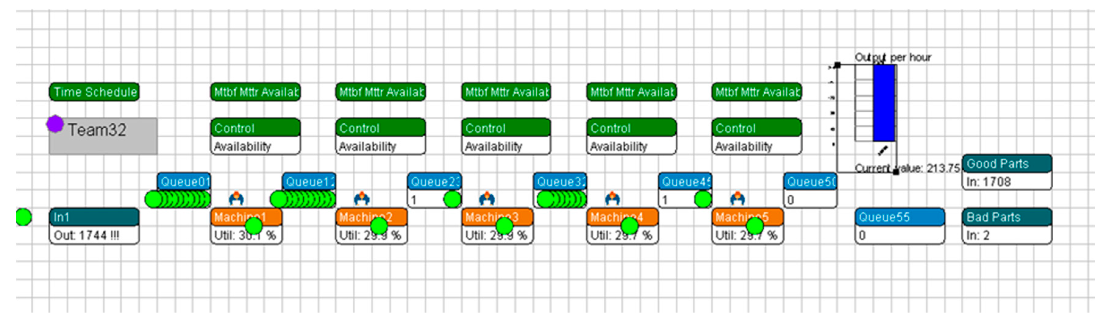
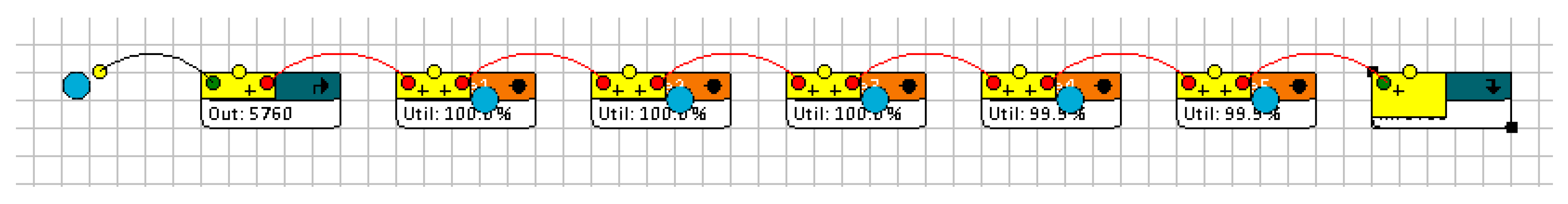
The first model, presented in Figure 2, is simply a reference model. It consists of five machines, an input and an output station. It represents production in ideal conditions and can be used for the calculation of the maximal production limit.

In the next step, additional elements were included in the model that represent constraints and noise factors (buffers, availability control, and time schedule).

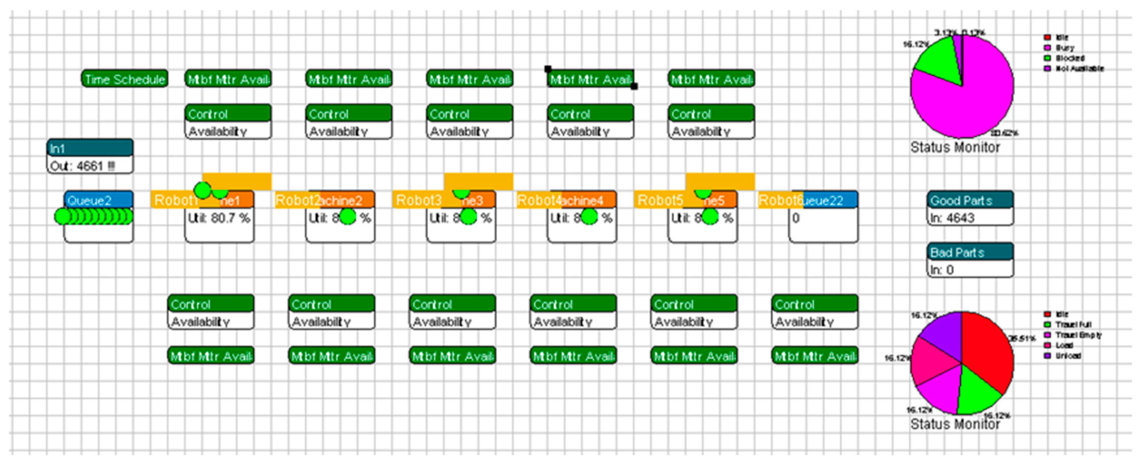
Parameters of a typical manufacturing process were taken into account, including a constant machine cycle time of 5 s as well as stochastic parameters of the operator time, which was described by normal distribution with a 10 s mean time and a 2 s standard deviation. On the other hand, robots have determined parameters, including a constant speed of 180°/s and a loading/unloading time of 1 s. Availability parameters include a planned setup time of 15 min per shift, and a rest break for workers of 15 min per shift. Failure parameters were taken into account, including a short-time human error rate and long-time machine and robot MTBF. Typical reliability parameters related mainly with equipment failures, include MTBFm = 500 h and MTTRm = 4 h for machines and MTBFr = 1000 h and MTTRr = 4 h for robots. Also, a normal quality distribution of good and bad products has been included in the model, which assumes 99.73% of good products for the model with human resources and 99.999% for the robotic line.

The second model, shown in Figure 3, includes five human operators, six buffers, and an output for good and bad quality products. The work time schedule is used for defining planned work pauses and additional MTBF objects that are used for simulation of random failures.

Irregular work of operators and human errors cause disturbances in the production process. In addition, human errors are possible and they are be described by parameters: MTBFh = 8 h and MTTRh = 5 min. We assume that another employee can replace a sick and absent worker, but it is impossible to replace broken machines and robots, and these require repairing.

The third model presented in Figure 4, includes industrial robots. Because of the constant speed and very regular work of robots, buffers are not needed.

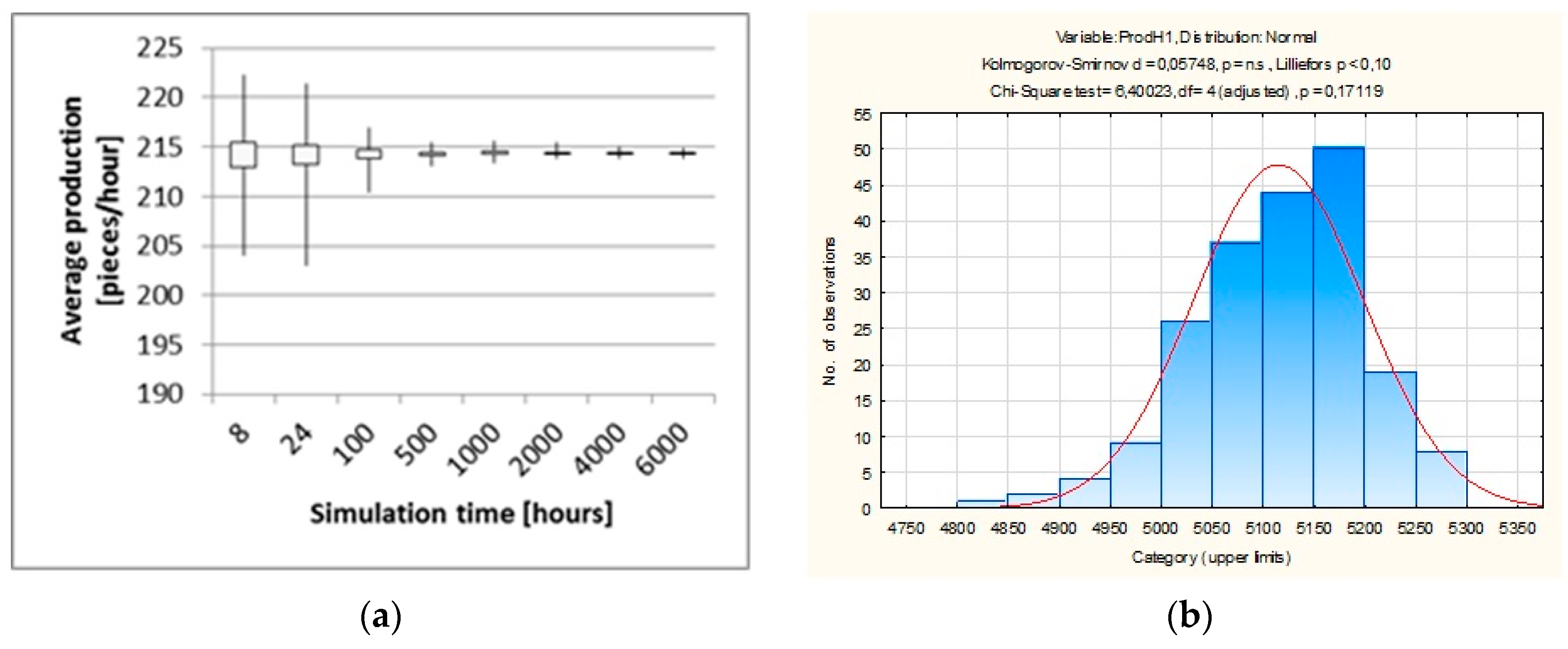
We can see a great improvement in the production throughput and machine utilization for the robotic line; however, each simulation run can give slightly different results because of random failures. Therefore, we have made a series of experiments containing different numbers of simulation runs and a simulation time ranging from 8 h to 6000 h.

5. Results

Simulation experiments were performed for the simulation time from the range of 8 to 6000 h (one, two and three shifts and 250 working days per year) in order to observe the influence of long-term failures. Each experiment consists of fifty samples (simulation runs).

The production value P obtained from one simulation is a random variable that consists of several parameters. The average production values P_avg of simulation experiments are summarized in

Table 1. Simulation results for manually operated and robotic lines (average production value P_avg in [PCs.] for 50 runs of simulation, α = 0.95, MTBFm = 500 h, MTBFr = 1000 h, MTTR = 4 h).

	Human	Robots	Human	Robots	Human	Robots	Human	Robots
	Operators		Operators		Operators		Operators
	MTBFm = 500 h MTBFr = 1000 h MTTR = 4 h		MTBFm = 500 h MTBFr = 1000 h MTTR = 4 h		MTBFm = 500 h MTBFr = 1000 h MTTR = 4 h		MTBFm = 500 h MTBFr = 1000 h MTTR = 4 h
	Time 8 h		Time 24 h		Time 2000 h		Time 6000 h
Max Limit [PCs.]	5760		17,280		1,440,000		4,320,000
Average Production Pavg [PCs.]	1681	4404	5111	13,300	427,179	1,094,949	1,281,345	3,279,888
Standard deviation [PCs.]	50.72	619.3	85.28	1432	714.96	19,331	1207	27,496
Relative deviation Δ	0.030	0.1406	0.0167	0.1077	0.0016	0.0176	0.0009	0.0084
OEE	0.2918	0.7646	0.2958	0.7697	0.2967	0.7604	0.2966	0.7592

. The value MaxLimit determines the maximum possible production volume in a given period of time at the ideal working conditions for a machine cycle time of Tm = 5 s.

Since the model was built based on the OEE components and contains parameters of availability, performance and quality, the production value from the simulation can be directly used to calculate the OEE indicator.

$$\mathrm{OEE}=\frac{\mathrm{Average}\mathrm{production}}{\mathrm{Maximal}\mathrm{production}\mathrm{limit}}$$

(9)

The random nature of the failures causes a significant dispersion of the obtained values and a relatively large standard deviation for the confidence level of α = 0.95.

The standard deviation shows the differences between the average value of production and the value of production achieved in each simulation run. For the robotically tended line, the values of standard deviation are also greater because of a much greater production volume and the possibility of robot failures. This phenomenon shows that absent humans can be replaced, but robots cannot.

The results of experiments with improved reliability parameters of machines and robots are summarized in

Table 2. Simulation results for manually operated and robotic lines (average production value P_avg in [PCs.] for 50 runs of simulation, α = 0.95, MTBFm = 1000 h MTBFr = 2000 h MTTR = 4 h).

	Human	Robots	Human	Robots	Human	Robots	Human	Robots
	Operators		Operators		Operators		Operators
	MTBFm = 1000 h MTBFr = 2000 h MTTR = 4 h		MTBFm = 1000 h MTBFr = 2000 h MTTR = 4 h		MTBFm = 1000 h MTBFr = 2000 h MTTR = 4 h		MTBFm = 1000 h MTBFr = 2000 h MTTR = 4 h
	Time 8 h		Time 24 h		Time 2000 h		Time 6000 h
Max Limit [PCs.]	5760		17,280		1,440,000		4,320,000
Average Production Pavg [PCs.]	1713	4540	5141	13,521	428,765	1,127,235	1,286,457	3,379,683
Standard deviation [PCs.]	35.76	440.2	84.09	967.6	662.4	12,068	1306	24,189
Relative deviation Δ	0.0207	0.0969	0.0164	0.0716	0.0015	0.0107	0.0010	0.0071
OEE	0.2974	0.7882	0.2975	0.7825	0.2978	0.7828	0.2978	0.7823

.

Relative deviation is a ratio between standard deviation and average production. It is decreasing with time and shows that the obtained results are more regular and the system is more stable. We can see that production throughput of the robotic line has increased about 2.6 times compared to the line before robotization.

The OEE related efficiency of a production line operated by a robot has improved by 48% compared to a manually operated line. The OEE indicator equals to OOEh = 29.18%–29.78% for humans and OEEr = 75.92%–78.23% for robots, and corresponds with the values assigned by the theory that are shown in

Table 3. Values of the OEE indicator.

Manufacturing Line	Human Operated Line OOEh	Robotic Line OEEr
Availability	0.893	0.938
Performance	0.333	0.833
Quality	0.9973	0.99999
OEE	0.297	0.782

. The values calculated by the theory are availability of the whole robotic system A = 0.938; performance P = 0.833; quality Q = 0.99999. That gives OEEr = 78.2%.

A reliability improvement can change the OEE score by about 2%. This shows that reliability parameters have a significant influence on the productivity of the production system. When comparing the OEE factors for a human operator and a robot, the greatest improvement is in the value of performance.

System Stability Analysis

In addition, the stability of the production system and the impact of failure parameters on the production throughput were analyzed in a similar manner as in the examples presented in [7]. Due to the random nature of a single failure process, a single simulation does not give a complete picture of the situation. Therefore, the experiment contains different numbers of simulation runs and a simulation time ranging from 8 h to 6000 h of work time. The trend lines of the average production value for the manually operated line and for the robotic line are presented in Figure 5a and Figure 6a, respectively.

In the box and whisker plot, the average value of production is in the “box” range with a confidence level of 95%. The “whiskers” show the minimum and maximum range of production value.

The trends of average production value are more stable for a longer simulation time. The model of the robotically tended line shows little difference compared to the model of the manually operated line. There are some outliers (the most extreme observations) represented by the minimum values of production that are connected with random failures and asymmetrical distribution with the left skewness (Figure 6b). On the other hand, almost symmetrical normal distribution can be observed in the case of manually operated lines (Figure 5b).

For a long simulation time, both models give results closer to normal distribution with smaller dispersion. These effects are related to the occurrence of irregular failures in short-time simulations and with the almost regular occurrence of failures for long-time simulations. Thus, the simulation time should be greater than or equal to the largest value of the MTBF parameter.

6. Conclusions

As it was predicted, the experiments confirm the advantage of the application of a robotic manufacturing line compared to a manually operated line. This is one of the best examples of robotic improvement in manufacturing. However, in other cases of machine tending, the difference between a human operator and a robot is not so clearly visible.

The computer simulation of the simplified model of the production line with machines, operators and robots with stochastic (short-time and long-time) reliability parameters allows for a better representation and understanding of a real production process. This is particularly visible in the case of work in three shifts per day for a long time period. The work organization and robot synchronization play an important role, and therefore the efficiency of the production line operated by robots has improved the OEE indicator by 48% compared to a manually operated line. Because of the irregular work of human operators, the buffers (queue) are needed for the equalization of production flow, and therefore loading (unloading) products from buffers results in a low performance of human operators. Also, breaks for rest result in a lower OEE value.

The use of the OEE indicator allows the comparison of the results from other manufacturing systems. The reality is that most manufacturing companies have OEE scores closer to 60%, but there are many companies with OEE scores lower than 40%, and a small number of world-class companies that have OEE scores higher than 80%. There are some areas for improvement of availability, performance and quality. Availability depends on planned and unplanned breaks at work. Performance score depends on the machine cycle time and the high robot speed. The quality depends on the stability of manufacturing process parameters.

The results obtained with the presented methodology can be used for the detailed design of a robotic system and for economic analysis, regarding labor costs and costs associated with the investments in robotization.