Grouped Bees Algorithm: A Grouped Version of the Bees Algorithm

Abstract

In many non-deterministic search algorithms, particularly those analogous to complex biological systems, there are a number of inherent difficulties, and the Bees Algorithm (BA) is no exception. The BA is a population-based metaheuristic search algorithm inspired by bees seeking nectar/pollen. Basic versions and variations of the BA have their own drawbacks. Some of these drawbacks are a large number of parameters to be set, lack of methodology for parameter setting and computational complexity. This paper describes a Grouped version of the Bees Algorithm (GBA) addressing these issues. Unlike its conventional version, in this algorithm bees are grouped to search different sites with different neighbourhood sizes rather than just discovering two types of sites, namely elite and selected. Following a description of the GBA, the results gained for 12 well-known benchmark functions are presented and compared with those of the basic BA, enhanced BA, standard BA and modified BA to demonstrate the efficacy of the proposed algorithm. Compared to the conventional implementations of the BA, the proposed version requires setting of fewer parameters, while producing the optimum solutions much more quickly.

1. Introduction

In recent years, we have considered many applications of population-based search algorithms in a diverse area of both theoretical and practical problems. Basically, these metaheuristic search algorithms are exceedingly well suited for optimization problems with a huge number of variables. Due to the nature of these multi variable problems, it is almost impossible to find a precise solution set for them within a polynomial bounded computation time. Therefore, swarm-based algorithms are preferred for finding the most optimal solution as much as possible within a sensible time. Some of the most well-known stochastic optimization methods are Ant Colony Optimization (ACO) [1], Artificial Bee Colony (ABC) algorithms [2], Biogeography-Based Optimization (BBO) [3], Genetic Algorithms (GA) [4], Particle Swarm Optimization (PSO) [5], the Cuckoo Search (CS) algorithm [6] and the Bees Algorithm (BA) [7].

The ACO algorithm mimics real ants’ behaviour in seeking food. Real ants generally wander arbitrarily to find food, and once it is found, they return to their colony while making a trail by spreading pheromone. If other ants face such a path, they will follow and reinforce the track, or revise it in some cases. Some theoretical and practical applications of ACO can be found in [8,9]. Some improvements for the search mechanism of ACO using derivative free optimization methods can be found in [10].

The ABC is another global optimization algorithm which is derived from the behaviour of honey bees while searching for food. For the first time, ABC was proposed in [2] for solving numerical optimization problems. The ABC has a colony model including three different groups of bees: employed, onlooker and scout. In the ABC, the employed bees are responsible for looking for new food resources rich with nutrients within the vicinity of the food resources that they have visited before [11]. Onlookers monitor the employed bees’ dancing and choose food resources based on the dances. Finally, the task of finding new food resources in a random manner is given to scout bees. The performance of ABC versus GA and PSO is evaluated by testing them on a set of multi variable optimization problems in [12]. In [13], the parameters of a feedforward neural network for classifying magnetic resonance (MR) brain images are optimized by a variant of ABC, called scaled chaotic ABC (SCABC). The performance of the SCABC algorithm is also compared against ABC, GA, and simulated annealing [14] in [13]. In [15], the ABC algorithm is used to select threshold values for image segmentation, where the ABC algorithm outperformed the GA and PSO algorithms. An example of the ABC application to increase throughput for wireless sensor networks is given in [16]. Regarding more recent variants of ABC, a velocity-based ABC (VBAC) algorithm is proposed in [17] where the onlooker bees apply the PSO search strategy to select the candidate solutions. An ABC algorithm based on information learning (ILABC) is proposed in [18], where a clustering partition is used to form subpopulation at each iteration to emphasize the exploitation process. A hybrid artificial bee colony (HABC) in proposed in [19], where the population size is dynamic based on a life-cycle model for the bees. In this method, a PSO-based comprehensive learning and a conjugate gradient descent search method is used for the exploitation of the search domain. A Migratory Multi-swarm Artificial Bee Colony (MiMSABC) is proposed in [20] where the bees are initially equally divided into some groups but with different perturbation mode. Gradually, as the algorithm proceeds, the subpopulation of each group may increase or decrease depending on the performance of each group. A comprehensive survey of many different types of bees optimization algorithms whether they are inspired by queen bees’ behaviour and mating, or foraging and communication of other bees is presented in [21].

The BBO algorithm, inspired from biogeography, is introduced by Dan Simon in 2008 [3]. In BBO, a solution is represented as an island including a number of species, i.e., independent input variables. A species migration probability is a function of the Habitat Suitability Index (HSI) of an island, i.e., the fitness of a solution. After a migration process, similar to other evolutionary algorithms, a mutation operation is applied on each input variable with some probability. A recent survey of the BBO algorithm can be found in [22].

The GA and PSO are two other well-known optimization algorithms which are inspired by two different biological approaches. The former works according to the evolutionary idea of the natural selection and genetics and the latter imitates the “social behaviour of bird flocking or fish schooling” [23]. The two techniques have been applied in a vast number of applications. As an example, in [24], GA is successfully used for calibrating the walking controller of a humanoid robot. Also, the performances of ACO, PSO, and GA on the radio frequency magnetron sputtering process are compared in [25]. A recent variant of the GA known as the “Quantum Genetic Algorithm” is reviewed in [26]. Regarding the PSO variants, a superior solution guided PSO (SSG-PSO) is proposed in [27] where a set of superior solutions are constructed for particles to learn from. In this variant, a mutation operation and gradient-based or derivative-free local search methods are employed. A scatter learning PSO algorithm (SLPSOA) is proposed in [28] where a pool of high-quality solutions are constructed as the exemplar pool. Each particle then selects an exemplar using a roulette wheel to update their position. An enhanced comprehensive learning particle swarm optimization (ECLPSO) is proposed in [29], where particles’ velocities have an additional perturbation term and use different exemplars for each dimension. A recent comprehensive survey on the PSO and its applications can be found in [30].

The CS, another meta-heuristic search algorithm, is introduced by Yang and Deb in 2009 [6]. This algorithm imitates the “obligate brood parasitic behaviour” of some cuckoos, which put their eggs in nests of other birds [31]. A solution is represented by an egg which can be found by another host bird with a specific likelihood. The host bird can then follow two policies: to toss the egg out, or to drop the nest in order to construct a new nest. As such, the highest quality nest will be transferred through the generations to keep the best solutions throughout the process. A review of the CS algorithm and its applications can be found in [32]. A conceptual comparison of the CS to ABC and PSO can be found in [33].

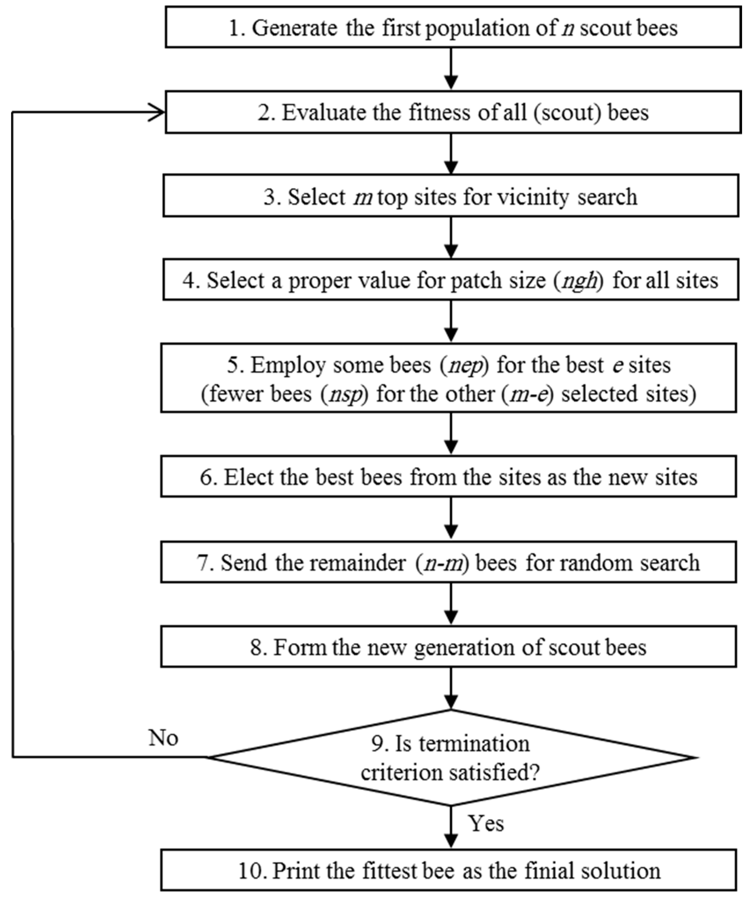
The BA is another optimization metaheuristic derived from the food-seeking behaviour of honey bees in nature. A detailed description of BA can be found in Section 2. A comprehensive survey and comparison of BA to ABC and PSO is presented in [34]. The basic BA and its other versions have been widely used in various problems including manufacturing cell formation [35], integer-valued optimizations for designing a gearbox [36], printed-circuit board (PCB) assembly configuration [37,38], machine job scheduling [39], adjusting membership functions of a fuzzy control system [40], neural network training [41], data clustering [42], automated quiz creator system [43], and channel estimation within a MC-CDMA (Multi-Carrier Code Division Multiple Access) communication system [44].

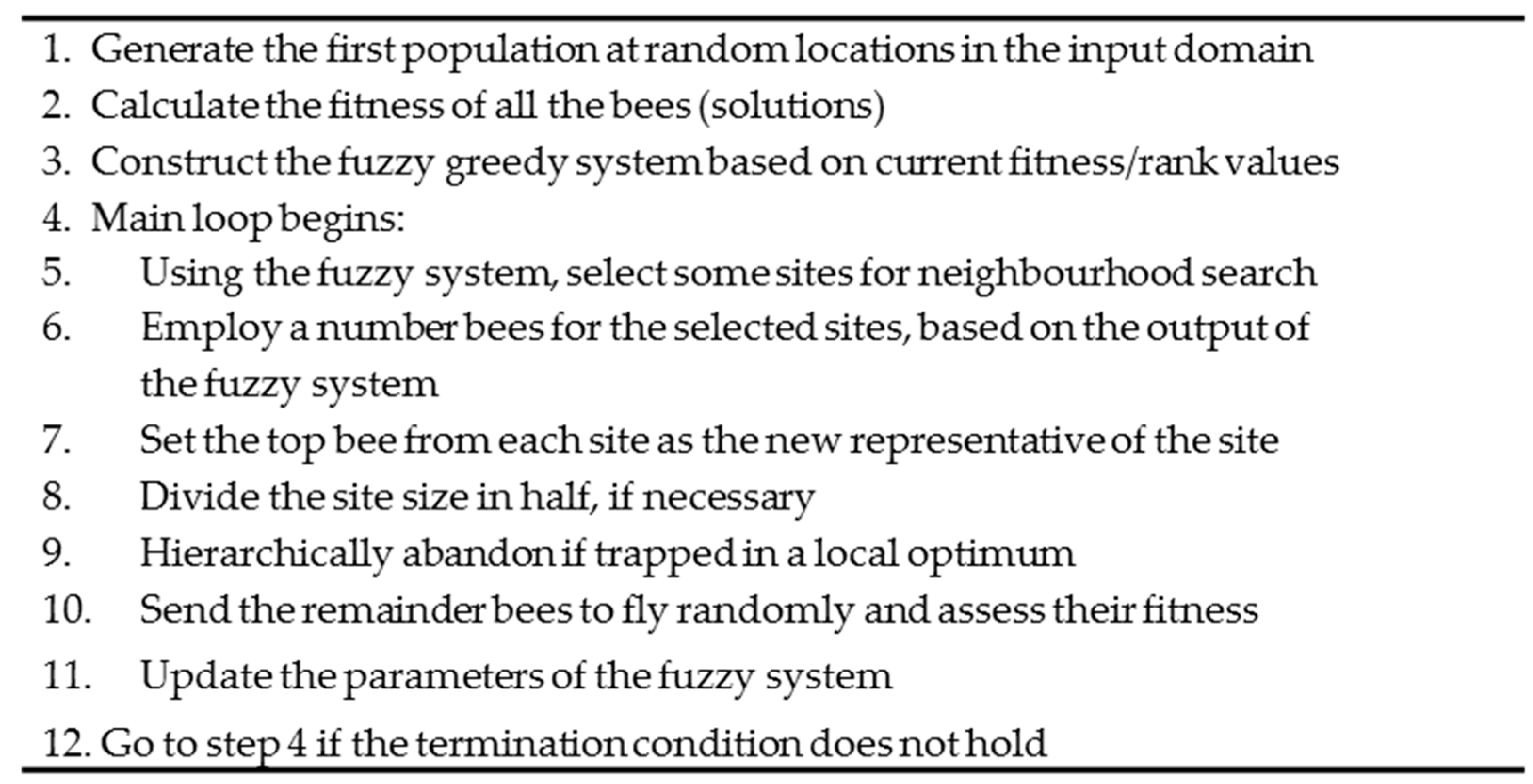
In the literature, various versions of BA such as enhanced BA, standard BA and modified BA are introduced after the basic BA. In [45], a fairly detailed review of many different versions of BA is presented. The enhanced BA has higher computational complexity because of its included fuzzy subsystem which selects potentially better sites or patches (i.e., solutions) for better exploration, though it reduces the number of setting parameters. The standard BA has increased the accuracy and speed by applying two new procedures on the basic version. This improvement has led to higher complexity for standard BA. In the modified BA, a collection of new operators is added to the basic BA, which results in a performance improvement, and consequently, too much more complexity compared to all the other versions. To compare the performance of the BA family with those of other population-based algorithms, such as GA, PSO or ACO, see [34,46,47]. Nevertheless, it is worth mentioning that, based on these studies, the Bees Algorithm family outperforms all the other population-based algorithms in continuous-variable optimization problems. As the benchmarks set used in these studies are exactly the same as the one in this paper, the performance of the proposed grouped bees algorithm is only compared against other BA variants.

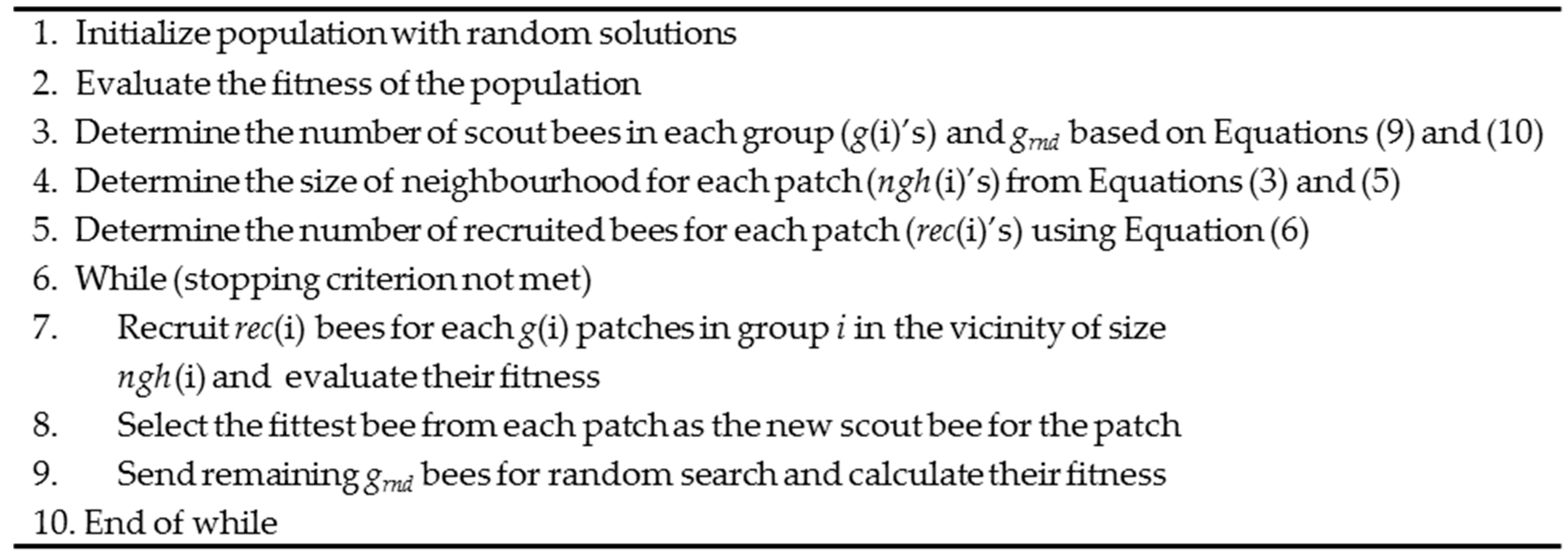
In this paper, a grouped version of the Bees Algorithm is introduced for multi-variable optimization problems. In this variant, bees are grouped into two or more search groups. In the first groups, more bees are recruited to search smaller but richer patches. In the last groups, more scout bees attempt to discover new patches within larger neighbourhoods. Well-defined formulas are used to set the parameters of the algorithm. Therefore, the number of adjustable parameters that has to be set is reduced. The original behaviour of the Bees Algorithm is maintained without any additional system or any extra operators. The remainder of this paper is organized as follows. The proposed Grouped Bees Algorithm (GBA) is elaborated in Section 2, where the core idea of the basic Bees Algorithm and its different modifications are also reviewed. In Section 3, the benchmark functions for evaluating the proposed algorithm and the performance of the algorithm on each of them are discussed. General interpretation of results in view of other BA variants and future research directions are given in Section 4. Finally, Section 5 summarizes the paper.

2. Materials and Methods

2.1. The Bees Algorithm

The Bees Algorithm, which imitates the natural food seeking behaviour of a swarm of honey bees, fits in the category of population-based optimization algorithms. Figure 1 shows the flowchart of the BA [48]. User needs to initialize a number of parameters before the algorithm begins the optimization process. These parameters are known as: the number of scout bees (n), number of selected sites out of n recently visited regions for neighbourhood search (m), number of elite sites out of m selected regions (e), number of recruited bees for the top e sites (nep), number of recruited bees for the remaining (m-e) selected regions (nsp), and finally, the initial size of each site (ngh) [7]. It is important to state that a site (or patch) represents an area in the search domain that contains the visited spot and its vicinity.

By initializing n scout bees in a random manner over the search space, the BA starts working in the first step, as shown in Figure 1. In the next step, the recently visited patches by the scout bees have to be assessed based on a predefined fitness function. In step 3, the m superior patches are labelled as selected patches for vicinity search. In the next step, step 4, an initial dimension of ngh for the patches is determined. The basic form of BA decreases the size of patches gradually to help search for a more accurate solution while the algorithm iteration advances [7]. The two groups of recruited bees probe near the chosen patches in the neighbourhood of radius ngh in step 5, and in step 6, the algorithm picks the top bee from each patch as the new representative of the patch. The remaining bees, in step 7, are the random search bees of the swarm to maintain stochastic nature of the algorithm. They are assigned to look for any new potential solutions by randomly flying over the search domain, and hopefully escaping from local minima. Next generation of the swarm will be formed by the random search bees of step 7 and the representative bees declared in step 6. A complete description of the basic BA can be found in [7,49].

Previous Modifications to the Bees Algorithm

The large number of parameters which should be set is a downside of the basic Bees Algorithm. Although some variations of the Bees Algorithm attempt to solve this issue, they do so at the expense of computational complexity. In [46] an enhanced version of the BA, employing two features of a fuzzy greedy system for selection of patches and a hierarchical abandonment method, is described. The abandonment method was first introduced by Ghanbarzadeh [50]. When the algorithm is stuck in a local optimum, this method triggers by removing the trapped site from the list of potential sites [50]. A hierarchical version of abandonment executes the same instruction on all sites with a lower rank than the trapped site [46]. The hierarchical version is utilized in the enhanced BA. A list of sorted candidate solutions based on their fitness determines the rank for each site. The Takagi–Sugeno fuzzy selection system decides the number of selected sites and the number of recruited bees for each site based on a greedy policy [46]. This fuzzy inference process needs to be executed in every iteration which may not be a favorable approach in an iterative algorithm.

Setting two parameters, the “number of scout bees” and the “maximum number of recruited bees for each site” is required in the enhanced BA [46]. The two parameters can have the same values, and the initial size of the sites’ neighbourhood (nh) is set to be a fraction of the size of the whole search domain. Figure 2 illustrates the pseudo-code of the Enhanced BA (EBA) [46].

To improve the search accuracy and computation performance, two other procedures are introduced in [51,52]. In the first approach, the search begins within the initial neighbourhood size of sites (nh) of the basic BA. It continues using the initial neighborhood size as long as the recruited bees are discovering better solutions in the neighbourhood. If the recruited bees fail to make any progress, the patch will become smaller. This procedure is called the “neighbourhood shrinking” method [51]. In [34], the heuristic formula for updating the size of neighbourhood for each input variable (nh) is stated as follows:

$$nh\left(0\right)=Max-Min$$

(1)

$$nh\left(t+1\right)=0.8\times nh\left(t\right)$$

(2)

where Max and Min indicate the maximum and minimum of the input vector respectively.

If shrinking the patch size does not result in any progress, the second procedure is applied. After a given number of loops, the patch is assumed to be trapped within a local minimum (or peak), and no further improvement would occur [34]. Therefore, the patch exploration is stopped and a new random patch is generated for hunting. This process is known as “abandoning sites without new information” [52] or “site abandonment” [34,52].

The basic version of PSO depends on the swarm’s best known position, and this feature leads the algorithm being potentially trapped in a local peak. This is an untimely convergence which can be avoided by including variable-size neighbourhood searches and random searches in the basic PSO algorithm to escape from stagnant states and reach a global optimum [53]. In the same current position and local best position case, a PSO particle would only escape from this point if the previous speed and inertia weight of the particle were non-zero. However, if previous velocities of the particles are around zero, all of them will stop searching when they reach this local peak, and this can lead to an immature convergence of the algorithm. This premature convergence problem of basic PSO is solved by proposing a hybrid version of PSO-BA in [53].

In [54], a different formulation for the Bees Algorithm is introduced by including new search operators and a new selection procedure which augment the survival probability of newly formed individuals. This improvement enhances the random search process of the Bees Algorithm using the following non-BA operators: mutation, creep, crossover, interpolation and extrapolation [54]. Every bee or solution has a chance for improvement by evolving a few times using the mentioned operators, and generation by generation the best bee is kept. At each step, a new evolutionary movement will only be accepted if any improvement is obtained; otherwise its current point will be retained. The number of these evolutionary operations on each solution decreases as the fitness quality of a solution decreases. This improved version strongly preserves the best bees. In addition, it keeps creating fresh bees and fostering them. Therefore, the large set of “best bees” would be reused to search again if they need to be [54].

More recently, a modified version of the Bees Algorithm is introduced in [28], which is mostly similar to the improved Bees Algorithm in [54], and in contrast to the basic BA, it requires many more parameters to be set. As such, a statistical method is offered to line up the extra parameters in [28]. In the Modified BA (MBA), new young solutions are preserved for a predetermined number of iterations from competition with more evolved bees. The overall performance of the MBA is evaluated by testing it on nine function benchmarks and comparing the results with that of other algorithms including standard BA, PSO, GA and so forth [47]. To the best of the authors’ knowledge, MBA has been the strongest version of the Bees Algorithm for single-objective problems to date, though at the expense of adding many complex operators.

Apart from the basic neighbourhood search method, two more methods are introduced in [55] to cope with multi-objective problems, where the “pareto” curve is formed by “all the non-dominated bees in each iteration.” During a simple neighbourhood hunt, a recruited bee is dispatched to a selected site and its fitness is calculated, and then its fitness is compared against the scout bee in the site. The old solution is replaced by the new one only if it could reach a fitter point in search space; otherwise it is not. Based on the first method, all the recruited bees, the number of which is nsp + nep, are sent to the selected site at the same time rather than one bee at a time. Then, the non-dominant bees are selected out of all the recruited bees considering their quality. Finally, the new scout bee will be selected for the site randomly, provided that there are at least two non-dominated bees. This approach is called “Random selection neighbourhood search”, and the second approach is named “Weighted sum neighbourhood search”, which is similar to the first random one. In fact, where the algorithm is deciding to choose the new scout bee by chance, a linear combination of the objective functions decides which “non-dominated bee” should replace the old scout in the site [56]. A brief overview of many bee-inspired algorithms, including both BA and ABC variants, can be found in [21].

2.2. The Proposed Grouped Bees Algorithm

The underlying idea behind the grouping concept is dividing all the particles into different categories for exploring the whole search space in a more structured approach. All the previous BA variants have two groups of elite and selected each of which searches the space by a different radius; the remainder particles, belonging to a third group, explore the environment randomly. As an understanding of the notion behind this metaphor, it can be said that the random search particles look for hopeful sites. Once any has been found, more precise particles (with smaller radiuses) are tasked with looking through the site for better solutions. The elite and selected groups look knowingly by different precisions as they exploit promising sites. In contrast, the random particles search unknowingly as they select a point in the search space haphazardly. This sudden jump in exploring from a knowing search to a completely unknowing search can take a longer time for complex high-dimensional domains. This issue of discontinuity in the search policy is tackled by the proposed Grouped Bees Algorithm (GBA) by implementing a spectrum of search from knowing to blind in a more continuous fashion.

The basic idea behind the proposed GBA is to implement a hierarchical search strategy which starts from a high-precision policy within small radiuses to a completely random one. The proposed Grouped Bees Algorithm (GBA) uses the basic Bees Algorithm as a core. The main difference between the basic BA and the grouped BA is the number of different patch types to be explored. This number in the basic BA is two, meaning there are always two types of selected patches, being either elite or good, whereas this number is essentially variable in GBA. In addition, this algorithm, unlike the basic BA, does not disregard any patch and searches all of them. In GBA, bees are grouped to search all the patches with different neighbourhood sizes. As such, it is no longer required to set the values of m, e, nep and nsp as the equivalent parameters for each group are determined based on mathematical relationships by the algorithm. The GBA has three parameters to be set: (1) the number of scout bees (n) which corresponds to the total number of patches (or sites) to be explored; (2) the number of strategical searching groups (groups); (3) the patch radiuses for the first group, containing top-rated scout bees (Ngh). These parameters and some other important notations of GBA are summarized in

Table 1. The nomenclature of the Grouped Bees Algorithm (GBA).

Parameter	Definition
n	Total number of scout bees *
groups	Total number of groups, excluding the random group *
i	Group number (index) starting from 1
j	Decision input variable index from 1 to m
g(i)	Number of scout bees (i.e., patches) in the i-th group
grnd	Number of scout bees for the random group, who are searching randomly
rec(i)	Number of recruited bees for patches in i-th group
Ngh	Radius vector of the neighbourhood for bees in the first group *
Ngh(i)	Radius vector of the neighbourhood for the i-th group
ngh(i)j	Radius for the j-th decision variable for bees in the i-the group

* To be set by user, whereas other parameters are automatically calculated.

.

The algorithm follows three general intuitive rules: (1) when a scout bee gets closer to the global optimum, a more precise and detailed exploration is needed, so the search neighbourhood size becomes smaller (for the groups with smaller indices) and vice versa; (2) based on the nature of honey bees [57,58], better flower patches, which generally corresponds to the groups with smaller indices, should be visited by more recruited bees; (3) the larger the neighbourhood size (radius), the more scout bees are needed to cover the whole area.

Similar to the BA mathematical notations [34], the input domain of all possible solutions is considered to be U = {X ∈ℝ^m; Min < X < Max}. So, assuming a fitness function is defined as f(X): U → R, each potential solution (bee) is formulated as an m-dimensional vector of input variables X = {x₁, ..., x_j, ..., x_m} where x_j is between min_j and max_j, corresponding to the decision variable number j. The search neighbourhood for the whole set of bees belonging to the same group of i is defined as an m-dimensional ball with the radius vector of Ngh(i) = {ngh(i)₁, ... ngh(i)_j, ..., ngh(i)_m} which is centered on the scout bees in the group i. In fact, each (recruited) bee will search on its own neighbourhood (patch), but the neighbourhood size is the same for all bees belonging to the same group. Now, considering the first rule, it is suggested each radius of ngh(i)_j should have the following relationship with the group number, i:

$$ngh{\left(i\right)}_j=a_j·i^2+b_j$$

(3)

subject to:

$$\{\begin{array}{l}Ngh=Ngh\left(1\right)=\left\{ngh{\left(1\right)}_1,..,ngh{\left(1\right)}_j,..,ngh{\left(1\right)}_m\right\}\hfill \\ ngh{\left(groups\right)}_j=\frac{ma{x}_j-mi{n}_j}{2}\hfill \end{array}$$

(4)

which yields:

$$\{\begin{array}{l}{a}_j=\frac{\left(\frac{ma{x}_j-mi{n}_j}{2}\right)-ngh{\left(1\right)}_j}{group{s}^2-1}\hfill \\ b_j=ngh{\left(1\right)}_j-a_j\hfill \end{array}$$

(5)

A simple equation for the number of recruited bees in each group, which is in line with the second rule, is decided to be:

$$\begin{array}{l}rec\left(i\right)={\left(groups+1-i\right)}^2\hfill \\ 1\le i\le groups\hfill \end{array}$$

(6)

Given the third rule, it is proposed that the number of scout bees in each group, g(i), should be proportional to the group index square, i², while the total number of all the scout bees who search either randomly or strategically should be equal to n. To that end, the area under the graph of k·x² over the interval [1, groups + 1] should sum up to n. So, the problem is finding a coefficient, k, which makes the definite integral of the function of f(x) = k·x² with respect to x from 1 to groups + 1 equal to n, i.e., to find k like so:

$${\displaystyle \underset{1}{\overset{groups+1}{{\displaystyle \int }}}}k·x^{2}dx=n$$

(7)

which results in:

$$k=\frac{3n}{{\left(groups+1\right)}^3-1}$$

(8)

Given the above, the algorithm determines the number of scout bees in each group as:

$$\{\begin{array}{l}g\left(i\right)=\lfloor k·i^2\rfloor \hfill \\ \mathrm{if}g\left(i\right)=0\mathrm{then}g\left(i\right)=1\hfill \end{array}$$

(9)

where k is given in Equation (8), and the number of scout bees for the random group, which seek randomly, is given by:

$$g_{rnd}={\left(n-{\displaystyle {\displaystyle \sum }_{i=1}^{groups}}g\left(i\right)\right)}^{+}$$

(10)

where x⁺ = max(x, 0). To reiterate, Figure 3 illustrates the pseudo code of the Grouped Bees Algorithm.

3. Results

In order to assess the performance (i.e., speed and accuracy) of the proposed GBA, the algorithm is applied to 12 well-known benchmark functions. The results are then compared to those reported in [7,46,47]. To assure a fair and unbiased comparison with other variants of BA, those algorithms were not implemented by us; rather, the best solutions claimed by their authors are considered. This is partially because every single benchmark function requires many attempts and parameters tweaked for each optimization algorithm. Therefore, only these 12 benchmark functions with reported performances (by their authors) are considered, whereas in some other studies the 25 benchmark functions set proposed in the special session on IEEE Congress on Evolutionary Competition (CEC) 2005 [59] or the benchmark functions set proposed for some other years of CEC is used. The basis of all these functions is the same as the benchmark functions used in this paper, though.

3.1. Benchmark Set

For each benchmark function, the interval of the input variables, the equation and the global optimum are shown in

Table 2. Benchmark Functions.

Function	Interval	Equation	Global
1. Martin & Gaddy 2D	[0, 10]	$\min f(x_1,x_2)= {(x_1-x_2)}^2+{(\frac{x_1+x_2-10}{3})}^2$	$$\begin{gathered} \overrightarrow{x}=(5,5) \\ f(\overrightarrow{x})=0 \end{gathered}$$
2. Branin 3D	[−5, 10]	$$\begin{gathered} \min f(x_1,x_2)= a(x_2-b{x_1}^2+c{x}_1- d) \\ +e(1-f)\cos (x_1)+e \\ a=1, b=\frac{5.1}{4}{(\frac{7}{22})}^2,c=\frac{5}{22}*7,d=6, e=10,f=\frac{1}{8}*\frac{7}{22} \end{gathered}$$	$$\begin{gathered} \overrightarrow{x}=(-\frac{22}{7},12.275) \\ \overrightarrow{x}=(\frac{22}{7},2.275) \\ \overrightarrow{x}=(\frac{66}{7},2.475) \\ f(\overrightarrow{x})=0.3977272 \end{gathered}$$
3. Rosenbrock 4D	[−1.2, 1.2]	$\min f(\overrightarrow{x})= {{\displaystyle \sum }}_{i=1}^3(100{({x_i}^2-x_{i+1})}^2+{(1-x_i)}^2$)	$$\begin{gathered} \overrightarrow{x}=(\overrightarrow{1}) \\ f(\overrightarrow{x})=0 \end{gathered}$$
4. Hypersphere 6D	[−5.12, 5.12]	$\min f(\overrightarrow{x})={\displaystyle {\displaystyle \sum }_{i=1}^6}{x_i}^2$	$$\begin{gathered} \overrightarrow{x}=(\overrightarrow{0}) \\ f(\overrightarrow{x})=0 \end{gathered}$$
5a. Rosenbrock 2D	[−10, 10]	$\min f(x_1,x_2)= 100{({x_1}^2-x_2)}^2+ {(1-x_1)}^2$	$$\begin{gathered} \overrightarrow{x}=(\overrightarrow{1}) \\ f(\overrightarrow{x})=0 \end{gathered}$$
5b. Rosenbrock 2D	[−1.2, 1.2]	$\min f(x_1,x_2)= 100{({x_1}^2-x_2)}^2+ {(1-x_1)}^2$	$$\begin{gathered} \overrightarrow{x}=(\overrightarrow{1}) \\ f(\overrightarrow{x})=0 \end{gathered}$$
5c. Rosenbrock 2D	[−2.048, 2.048]	$\max f(x_1,x_2)=(3905.93)- 100{({x_1}^2-x_2)}^2- {(1-x_1)}^2$	$$\begin{gathered} \overrightarrow{x}=(\overrightarrow{1}) \\ f(\overrightarrow{x})=3905.93 \end{gathered}$$
6. Goldstein & Price 2D	[−2, 2]	$$\begin{gathered} \min f(x_1,x_2)= A(x_1,x_2)B(x_1,x_2) \\ \begin{array}{c}A(x_1,x_2)=1+{(x_1+x_2+1)}^2(19-14x_1+3{x_1}^2\\ -14x_2+6x_1{x}_2+3{x_2}^2)\end{array} \\ \begin{array}{c}B(x_1,x_2)=30+{(2x_1-3x_2)}^2(18-32x_1+12{x_1}^2\\ +48x_2-36x_1{x}_2+27{x_2}^2)\end{array} \end{gathered}$$	$$\begin{gathered} \overrightarrow{x}=(0,-1) \\ f(\overrightarrow{x})=3 \end{gathered}$$
7. Schwefel 6D	[−500, 500]	$\max f(\overrightarrow{x})={\displaystyle {\displaystyle \sum }_{i=1}^6}{x}_i\sin (\sqrt{\left|x_i\right|})$	$$\begin{gathered} \overrightarrow{x}=(\overrightarrow{420.9687}) \\ f(\overrightarrow{x})\approx -2513.9 \end{gathered}$$
8. Shekel Foxholes 2D *	[−65.536, 65.536]	$\min f(x_1,x_2)=-{\displaystyle {\displaystyle \sum }_{j=1}^{25}}\frac{1}{j+{(x_1-A_{1j})}^6+{(x_2-A_{2j})}^6}$	$$\begin{gathered} \overrightarrow{x}=(-32,-32) \\ f(\overrightarrow{x})\approx -1 \end{gathered}$$
9. Steps 5D	[−5.12, 5.12]	$\min f(\overrightarrow{x})={\displaystyle {\displaystyle \sum }_{i=1}^5}\mathrm{int}(x_i)$	$$\begin{gathered} \overrightarrow{x}\in \overrightarrow{\left[-5.12,-5\right]} \\ f(\overrightarrow{x})=-25 \end{gathered}$$
10. Rosenbrock 5D	[−2.48, 2.48]	$\min f(\overrightarrow{x})= {{\displaystyle \sum }}_{i=1}^4(100{({x_i}^2-x_{i+1})}^2+{(1-x_i)}^2$)	$$\begin{gathered} \overrightarrow{x}=(\overrightarrow{1}) \\ f(\overrightarrow{x})=0 \end{gathered}$$
11. Griewangk 10D	[−600, 600]	$\min f(\overrightarrow{x})=\frac{1}{4000}.{\displaystyle {\displaystyle \sum }_{i=1}^{10}}{x_i}^2-{\displaystyle {\displaystyle \prod }_{i=1}^{10}}\cos (\frac{x_i}{\sqrt{i}})+1$	$$\begin{gathered} \overrightarrow{x}=(\overrightarrow{0}) \\ f(\overrightarrow{x})=0 \end{gathered}$$
12. Rastrigin 20D	[−5.12, 5.12]	$\min f(\overrightarrow{x})={\displaystyle {\displaystyle \sum }_{i=1}^{20}}({x_i}^2-10\cos (2\pi x_i)+10)$	$$\begin{gathered} \overrightarrow{x}=(\overrightarrow{0}) \\ f(\overrightarrow{x})=0 \end{gathered}$$

* Coefficients Aij in Shekel function as defined in Adorio (2005) [61].

as reported in [60,61]. The Martin & Gaddy and Hypersphere benchmarks are uni-modal functions which are quite straightforward for optimization tasks. The Branin function has three global optima with exactly the same value. The minimum of the unimodal Rosenbrock function is at the lowest part of a long and narrow valley [34]. While the valley can be simply discovered within a few repetitions of an optimization algorithm, locating the exact global minimum is quite difficult. The Goldstein & Price function is also an easy benchmark for optimization with only two input parameters. The Schwefel function is quite misleading where the global minimum is distant from the second best minimum [60]. As such, the optimization algorithms could easily fall into the trapped second best minimum. The multi-modal Shekel function has a complex search space. The Steps benchmark is formed of many flat plateaus and steep ridges. The Griewangk and Rastrigin functions are extremely multi-modal. Both functions include a cosine modulation creating numerous local minima. Yet the locations of the local minima throughout the search space are regularly spread [60].

3.2. Speed Evaluation

As the first experiment, the proposed algorithm was tested for speed, and compared to the basic BA [7] and the enhanced BA on the benchmark functions from 1 to 7. The experiment conditions were set according to the experiments of Pham and his colleagues [34,46]. Accordingly, the grouped Bees Algorithm was run 100 times, with different random initializations, for each of these functions. The error for the while-loop of the GBA was defined as the difference between the value of the global optimum and the fittest solution found by the GBA, at each iteration. The optimization procedure then stopped when the error was less than 0.001 times the minimum of one and the global optimum. When the optimum value was zero, the procedure stopped if the solution was different from the optimum value by less than 0.001. From a mathematical perspective, the stopping criteria were hence set to be:

$$error=f\left(x\right)-f^{*}$$

(11)

$$stoppingcriterion=\{\begin{array}{ll}error\le 0.001\hfill & ;f^{*}=0\hfill \\ error\le min\left(0.001,0.001f^{*}\right)\hfill & ;f^{*}\ne 0\hfill \end{array}$$

(12)

where f(x) is the value of the benchmark function f at the input point of x, and f* is the value of its global optimum.

Table 3. Mean number of evaluations of functions 1–7 for BA, EBA [46] and GBA.

Function	Mean Number of Evaluations
	Basic BA	Enhanced BA	Grouped BA
1. Martin & Gaddy 2D	526	124	114
2. Branin 3D	1657	184	216
3. Rosenbrock 4D	28,529	33,367	29,601
4. Hypersphere 6D	7113	526	565
5a. Rosenbrock 2D	2306	1448	1026
5b. Rosenbrock 2D	631	689	580
5c. Rosenbrock 2D	868	830	679
6. Goldstein & Price 2D	999	212	273
7. Schwefel 6D	Approx. 3 × 106	N/A	Approx. 1 × 106

presents the results of applying the basic BA and the enhanced BA to the same benchmark suite as reported in [7,46]. The table shows the average number of function evaluations performed by the GBA before it stops due to the same stopping criterion for all the algorithms. For each benchmark problem, the best result is emphasised in bold. By looking at the table, it is immediately clear that the GBA outperformed the basic method. However, to provide more comparable figures,

Table 4. Differences in the average number of evaluations.

Function	Percentage Change in GBA w.r.t.
	Basic BA	Enhanced BA
1. Martin & Gaddy 2D	−78.33%	−8.06%
2. Branin 3D	−86.96%	17.39%
3. Rosenbrock 4D	3.76%	−11.29%
4. Hypersphere 6D	−92.06%	7.41%
5a. Rosenbrock 2D	−55.51%	−29.14%
5b. Rosenbrock 2D	−8.08%	−15.82%
5c. Rosenbrock 2D	−21.77%	−18.19%
6. Goldstein & Price 2D	−72.67%	28.77%
Average	−51.45%	−3.62%

details the difference between the total numbers of fitness function calculations done by each algorithm compared to the GBA’s. This figure is expressed for each function as the percentage change in the mean numbers of evaluations by the GBA with respect to those by the other algorithms. As shown in Table 4, the GBA is nearly two times faster than the basic BA, whereas its convergence speed is generally as fast as the enhanced BA. To statistically confirm the first claim, a multiple-problem non-parametric test is performed as suggested in [62]. A non-parametric test is preferred since it does not make assumptions regarding the data, as opposed to parametric tests. The performances of the basic BA and GBA are represented by the mean number of evaluations in each function (or benchmark problem). An alpha (α) value of 0.5 is considered for the statistical tests. A Wilcoxon signed-rank test shows a statistically significant change in the number of evaluations from the basic BA to GBA over the set of benchmark problems (Z = −2.703, p = 0.039). However, the difference between the number of evaluations performed by the basic BA and GBA does not seem to have a quite symmetric distribution. This is partially due to the fact that benchmark problems are completely different from one another. Therefore, a paired-samples sign test, which is not sensitive to the normality assumption, is performed to be on the safe side. An exact sign test also resulted in statistically significant median decrease in the number of evaluations by GBA compared to the basic BA, p = 0.039. It is notable that the data regarding each run of the basic BA and the enhanced BA are not available from either reference [34] or reference [46]. As such, single-problem statistical analysis (i.e., comparing runs for each benchmark function) is not possible.

The obvious difference between the enhanced BA and the GBA is the high computational costs of employing the enhanced BA, which heavily depends on its fuzzy subsystem in all the iterations. Therefore, the GBA is far more computationally efficient than the enhanced BA. In addition, in Figure 4 the search strategy for finding the optimal point of GBA and the enhanced BA [46] are depicted for the Shekel function. The dashed red line and dashed greenish-blue line show the GBA’s best point evolution track and the enhanced BA’s best point evolution track, respectively. As shown in this figure, GBA has a greedier policy to reach the best point in short pieces of time compared to the enhanced BA. In other words, in GBA, each bee tries to reach the best point within their neighbourhood in as few iterations as possible, and it is not an issue to be trapped in a local optimum point. That is, a bee does not have to be worried about local optima, as those bees belonging to the higher groups, with larger patch sizes, have enough chances of being located in the route toward the global optimum point. So, the GBA’s best solution has considerably less jumping in the search space than the enhanced BA. It is evident that the enhanced BA jumps much more over the search space. This is because of its strategy encountering local points i.e., site abandonment. Though site abandonment could release the trapped bee from local optima, yet it leads to a generally slower process in finding the optimum. In the end, it can be stated that GBA exhibits more evolutionary intelligence than the enhanced BA in reaching the optimum point. The parameters used by the GBA for benchmark functions from 1 to 7 in this experiment can be found in

Table 5. The parameters used by GBA in the speed experiment. * The Ngh vector has the same scalar value in all dimensions.

Function	n	Groups	Ngh *
1. Martin & Gaddy 2D	6	3	0.13
2. Branin 3D	8	3	0.05
3. Rosenbrock 4D	4	3	0.001
4. Hypersphere 6D	4	3	0.035
5a. Rosenbrock 2D	5	3	0.11
5b. Rosenbrock 2D	6	3	0.08
5c. Rosenbrock 2D	4	3	0.09
6. Goldstein & Price 2D	9	3	0.006
7. Schwefel 6D	500	3	0.2

.

3.3. Accuracy Evaluation

As the second experiment, the proposed algorithm is tested for accuracy, and compared to the standard BA [34] and the modified BA [47] on the benchmark functions from 5c to 12. The standard BA is a better version of the basic BA which employs neighbourhood shrinking and site abandonment methods [34]. The stopping criteria in this experiment are defined differently form the first experiment. The experiment conditions were set according to the experiments in [47]. This means the grouped Bees Algorithm was run independently 20 times, as was an experimental condition in [47]. By the end of each run, the fittest bee of the last iteration was considered to be the final solution. For each benchmark problem, the exact number of iterations was preset in such a way that the number of function evaluations was as close as possible to that of the standard Bees Algorithm or the modified BA in [47], whichever was smaller. From a mathematical point of view, Equations (13)–(15) show how to calculate the exact number of iterations and function evaluations in the GBA.

The number of evaluations in one iteration (λ) of GBA is defined as:

$$\lambda ={\displaystyle {\displaystyle \sum }_{i=1}^{groups}}g\left(i\right)·rec\left(i\right)+g_{rnd}$$

(13)

As a result, the number of iterations, $\zeta$, and the number of evaluations, $\xi$, are obtained as:

$$\zeta =\lfloor \raisebox{1ex}{$\delta $}\!\left/ \!\raisebox{-1ex}{$\lambda $}\right.\rfloor$$

(14)

$$\xi =\zeta ·\lambda$$

(15)

where δ is the minimum number of evaluations in the standard BA and the modified BA.

The number of iterations and function evaluations for the three mentioned algorithms are provided in

Table 6. No. of iterations and evaluations by Grouped BA, Standard BA and Modified BA.

Function	Grouped BA		Standard BA			Modified BA
	Eval.	Iter.	Eval.	Iter.	Diff.%	Eval.	Iter.	Diff.%
5c. Rosenbrock 2D	480	32	494	19	2.92%	503	50	4.79%
6. Goldstein & Price 2D	1020	51	1040	40	1.96%	1026	100	0.59%
7. Schwefel 6D	1972	16	2002	77	1.52%	2011	200	1.98%
8. Shekel Foxholes 2D	988	19	1040	40	5.26%	1026	100	3.85%
9. Steps 5D	120	8	130	5	8.33%	126	10	5%
10. Rosenbrock 5D	1012	11	1040	40	2.77%	1026	100	1.38%
11. Griewangk 10D	1020	68	1040	40	1.96%	1026	100	0.59%
12. Rastrigin 20D	1015	35	1040	40	2.46%	1026	100	1.08%

Eval.: Evaluations; Iter.: Iterations; Diff.%: Difference%.

. The table shows the differences in the number of function evaluations between GBA and the other two algorithms in percentages. The absolute distance from the fitness of the final solution to the global optimum is denoted as the absolute error as is in [47]. Alike to [47], for each algorithm, the average and the median of absolute error are given in

Table 7. Mean and median of absolute error for Grouped BA, Standard BA and Modified BA.

Function	Grouped BA		Standard BA		Modified BA
	Mean	Median	Mean	Median	Mean	Median
5c. Rosenbrock 2D	0.0019	0.0002	0.0224	0.0078	0.0014	0.0003
6. Goldstein & Price 2D	0.0000	0.0000	0.0000	0.0000	0.0011	0.0000
7. Schwefel 6D	453.2246	454.0311	620.3443	572.2723	93.0656	73.4942
8. Shekel Foxholes 2D	0.2397	0.0000	0.0213	0.0095	0.1525	0.0000
9. Steps 5D	2.1500	2.0000	4.2000	4.5000	3.8500	4.0000
10. Rosenbrock 5D	1.3319	1.1019	1.2090	1.3728	1.3038	0.854
11. Griewangk 10D	0.9297	0.9483	1.0774	1.0887	1.0774	1.0718
12. Rastrigin 20D	83.6515	79.322	116.2691	120.6735	83.7651	77.871
Wins	5		3		3

. These numbers are displayed in decimal to an accuracy of 4 decimal places. The least errors obtained for each benchmark function are emphasised in bold. If two algorithms performed similarly, their results are both displayed in bold.

Table 8. The parameters used by GBA in the accuracy experiment. * The Ngh vector has the same scalar value in all dimensions.

Function	n	Groups	Ngh *
5c. Rosenbrock 2D	4	3	0.2
6. Goldstein & Price 2D	9	3	0.006
7. Schwefel 6D	20	6	0.5
8. Shekel Foxholes 2D	40	2	0.3
9. Steps 5D	4	3	3
10. Rosenbrock 5D	7	6	0.02
11. Griewangk 10D	4	3	10
12. Rastrigin 20D	15	3	0.025

shows the parameters used by the GBA for benchmark functions from 5c to 12 in the accuracy experiment.

According to Table 7, each of the grouped BA, modified BA and standard BA has been successful in achieving the minimum error in, respectively, five, three and three functions out of eight benchmarks. Considering both the mean and median errors, the grouped BA and the modified BA have performed almost equally in general. However, the standard BA has an equal or worse performance than the GBA in six benchmark functions out of eight. Once again, in order to add strength to these claims a number of non-parametric tests are performed as suggested in [62]. Unfortunately, the data regarding each run of standard BA and modified BA is not reported in [47]. Therefore, only multiple-problem statistical tests are conducted where the performance of the algorithms on each benchmark function is aggregated in a single number (e.g., mean/median error). The median error as reported in Table 7 is used as the representative for the performance of each algorithm in each function. The median is chosen over the mean as it is resistant to outliers and the violation of the normality assumption. First a Friedman test is carried out to see if there are any meaningful differences between the algorithms. At an alpha level of 0.05, the Friedman test confirms the existence of a statistically significant difference in the median error obtained by different BA variants, χ2(2) = 10.889, p = 0.002. Now in order to find where this significant difference lies, a post hoc analysis with Wilcoxon signed-rank tests is performed on all pairs of the BA variants. A Bonferroni correction of the alpha values results in a new significance level set at p < 0.017. There are no significant differences between the modified BA and the GBA (Z = −0.524, p = 0.688). However, there is a statistically significant reduction in error rate by the GBA vs. the standard BA (Z = −2.366, p = 0.016).

4. Discussion

To summarize the above-mentioned experiments, GBA not only is substantially faster than the basic version of BA, it also has a higher accuracy than the standard BA and a similar accuracy to the complex modified BA. It is notable that the modified BA is not considered to be one of the main implementations of the Bees Algorithm [45]. The modified BA may be considered to be a hybrid kind of BA that employs various operators including mutation, crossover, interpolation and extrapolation; whereas the GBA is not introducing any new operator to the basic BA, and has significantly less conceptual and computational complexity compared to all the other variants built on top of the basic BA.

As mentioned, the performance of GA, PSO, and ACO on exactly the same benchmark functions, used in this paper, can be found in [34,46,47]. In addition to the mathematical functions discussed here, GBA has shown great performance in two other applications. It was used for calibrating the parameters of a scripted AI in a boxing simulation game [63] where the fuzzy AI could not defeat the scripted AI after the GBA-based calibration procedure. GBA was also used to tune up the parameters of a hybrid controller for bipedal walking [64]. The parameters were adjusted in a way that a trajectory generator module, as a subsystem of the hybrid controller, produced stable walking trajectories.

The notion of grouping is to organize all the particles hierarchically so that the degree of awareness of a group search decreases by increasing their group number. This is achieved by increasing the search neighborhood for later groups in order to have a spectrum of groups by different precisions in the exploration strategy. Although basic BA and some of its variants suffer from discontinuity more than other metaheuristics like GA and PSO, it is possible to generalize the concept of grouping for other population-based algorithms. In GA, for example, the whole population could be divided into several groups by the same policy as GBA, and a freedom factor for each group should be considered. The freedom factor of each group would define the freedom degree of the new child produced by selected parents. In other words, it determines how much a new solution is allowed to move through search space by a GA operator such as crossover or mutation. Clearly, as group number increases, the freedom degree raises. The same policy can be applied on PSO and so on in order to implement the idea of grouping.

A further extension of this work focuses on comparing and discussing the performance of GBA against the genetics algorithm and simulated annealing on optimizing discreet input space and combinatorial problems such as travelling salesman problem and component placement problem, initially discussed in [14]. Moreover, the proposed GBA could be compared against a number of more recent advances in the metaheuristics optimization literature in high-dimensional problems.

5. Conclusions

In this study, the basic version of the Bees Algorithm has been restructured to improve its performance while decreasing the number of setting parameters. The proposed version is called the Grouped Bees Algorithm (i.e., GBA). In contrast to the basic Bees Algorithm, in GBA the bees are grouped to search different patches with various neighbourhood sizes. The group with the lowest index contains the fittest scout bees. This group has also the highest number of recruited bees. As the index of a group increases, the quality of the patches is reduced, and more scout bees are required to discover alternative potential solutions. There is also a random search group with at least one scout bee to preserve the stochastic nature of the algorithm.

The efficiency of the algorithm is assessed with two criteria: converging speed and accuracy. The algorithm is applied to 12 well-known function benchmarks. The net result indicates that the proposed variant is two times faster than the conventional Bees Algorithm, while almost as accurate as the more complex modified BA. Other desirable characteristics of the algorithm can be summarized as follows: (1) The grouped BA (GBA) has a well-defined methodology to set parameters, which leads to a lower number of tunable parameters; (2) The algorithm entails the least computational load; (3) It is based only on the conventional operators of the Bees Algorithm, i.e., the waggle dance.

References

1. Dorigo, M.; Stutzle, T. Ant Colony Optimization; MIT Press: Cambridge, MA, USA, 2004. [Google Scholar]
2. Karaboga, D. An Idea Based On Honey Bee Swarm for Numerical Optimization; Erciyes University: Kayseri, Turkey, 2005. [Google Scholar]
3. Simon, D. Biogeography-Based Optimization. IEEE Trans. Evol. Comput. 2008, 12, 702–713. [Google Scholar] [CrossRef]
4. Goldberg, D.E. Genetic Algorithms in Search, Optimization, and Machine Learning; Addison-Wesley Longman Publishing Co., Inc.: Boston, MA, USA, 1989. [Google Scholar]
5. Kennedy, J.; Eberhart, R. Particle swarm optimization. In Proceedings of the International Conference on Neural Networks (ICNN′95), Perth, Australia, 27 November–1 December 1995; Volume 4, pp. 1942–1948.
6. Yang, X.-S.; Suash Deb, S. Cuckoo Search via Lévy flights. In Proceedings of the 2009 World Congress on Nature & Biologically Inspired Computing (NaBIC), Coimbatore, India, 9–11 December 2009; pp. 210–214.
7. Pham, D.T.; Ghanbarzadeh, A.; Koc, E.; Otri, S.; Rahim, S.; Zaidi, M. The bees algorithm, a novel tool for complex optimisation problems. In Proceedings of the 2nd International Virtual Conference on Intelligent Production Machines and Systems (IPROMS), 3–14 July 2006; pp. 454–459.
8. Fogarty, T.C.; Parmee, I.C. Evolutionary computing. In Proceedings of the AISB Workshop, Sheffield, UK, 3–4 April 1995.
9. Mathur, M.; Karale, S.B.; Priye, S.; Jayaraman, V.K.; Kulkarni, B.D. Ant Colony Approach to Continuous Function Optimization. Ind. Eng. Chem. Res. 2000, 39, 3814–3822. [Google Scholar] [CrossRef]
10. Rebaudo, F.; Crespo-Perez, V.; Silvain, J.-F.; Dangles, O. Agent-Based Modeling of Human-Induced Spread of Invasive Species in Agricultural Landscapes: Insights from the Potato Moth in Ecuador. J. Artif. Soc. Soc. Simul. 2011, 14, 1–22. [Google Scholar] [CrossRef]
11. Karaboga, D.; Basturk, B. On the performance of artificial bee colony (ABC) algorithm. Appl. Soft Comput. 2008, 8, 687–697. [Google Scholar] [CrossRef]
12. Karaboga, D.; Basturk, B. A powerful and efficient algorithm for numerical function optimization: Artificial bee colony (ABC) algorithm. J. Glob. Optim. 2007, 39, 459–471. [Google Scholar] [CrossRef]
13. Zhang, Y.; Wu, L.; Wang, S. Magnetic Resonance Brain Image Classification by an Improved Artificial Bee Colony Algorithm. Prog. Electromagn. Res. 2011, 116, 65–79. [Google Scholar] [CrossRef]
14. Kirkpatrick, S.; Gelatt, C.D.; Vecchi, M.P. Optimization by simulated annealing. Science 1983, 220, 671–680. [Google Scholar] [CrossRef] [PubMed]
15. Zhang, Y.; Wu, L. Optimal Multi-Level Thresholding Based on Maximum Tsallis Entropy via an Artificial Bee Colony Approach. Entropy 2011, 13, 841–859. [Google Scholar] [CrossRef]
16. Singh, A.; Nagaraju, A. An Artificial Bee Colony-Based COPE Framework for Wireless Sensor Network. Computers 2016, 5, 2. [Google Scholar] [CrossRef]
17. Imanian, N.; Shiri, M.E.; Moradi, P. Velocity based artificial bee colony algorithm for high dimensional continuous optimization problems. Eng. Appl. Artif. Intell. 2014, 36, 148–163. [Google Scholar] [CrossRef]
18. Gao, W.-F.; Huang, L.-L.; Liu, S.-Y.; Dai, C. Artificial Bee Colony Algorithm Based on Information Learning. IEEE Trans. Cybern. 2015, 45, 2827–2839. [Google Scholar] [CrossRef] [PubMed]
19. Ma, L.; Zhu, Y.; Zhang, D.; Niu, B. A hybrid approach to artificial bee colony algorithm. Neural Comput. Appl. 2016, 27, 387–409. [Google Scholar] [CrossRef]
20. Biswas, S.; Das, S.; Debchoudhury, S.; Kundu, S. Co-evolving bee colonies by forager migration: A multi-swarm based Artificial Bee Colony algorithm for global search space. Appl. Math. Comput. 2014, 232, 216–234. [Google Scholar] [CrossRef]
21. Rajasekhar, A.; Lynn, N.; Das, S.; Suganthan, P.N. Computing with the collective intelligence of honey bees—A survey. Swarm Evol. Comput. 2017, 32, 25–48. [Google Scholar] [CrossRef]
22. Guo, W.; Chen, M.; Wang, L.; Mao, Y.; Wu, Q. A survey of biogeography-based optimization. Neural Comput. Appl. 2016, 1–18. [Google Scholar] [CrossRef]
23. Saini, S.; Awang Rambli, D.R.; Zakaria, M.N.B.; Sulaiman, S. A Review on Particle Swarm Optimization Algorithm and Its Variants to Human Motion Tracking. Math. Probl. Eng. 2014, 2014, 704861. [Google Scholar] [CrossRef]
24. Massah Bavani, A.; Ahmadi, H.; Nasrinpour, H.R. A closed-loop Central Pattern Generator approach to control NAO humanoid robots’ walking. In Proceedings of the 2nd International Conference on Control, Instrumentation and Automation, Shiraz, Iran, 27–29 December 2011; pp. 1036–1041.
25. Mohd Sabri, N.; Md Sin, N.D.; Puteh, M.; Mahmood, M.R. Optimization of Nano-Process Deposition Parameters Based on Gravitational Search Algorithm. Computers 2016, 5, 12. [Google Scholar] [CrossRef]
26. Lahoz-Beltra, R. Quantum Genetic Algorithms for Computer Scientists. Computers 2016, 5, 24. [Google Scholar] [CrossRef]
27. Wu, G.; Qiu, D.; Yu, Y.; Pedrycz, W.; Ma, M.; Li, H. Superior solution guided particle swarm optimization combined with local search techniques. Expert Syst. Appl. 2014, 41, 7536–7548. [Google Scholar] [CrossRef]
28. Ren, Z.; Zhang, A.; Wen, C.; Feng, Z. A Scatter Learning Particle Swarm Optimization Algorithm for Multimodal Problems. IEEE Trans. Cybern. 2014, 44, 1127–1140. [Google Scholar] [PubMed]
29. Yu, X.; Zhang, X. Enhanced comprehensive learning particle swarm optimization. Appl. Math. Comput. 2014, 242, 265–276. [Google Scholar] [CrossRef]
30. Zhang, Y.; Wang, S.; Ji, G. A Comprehensive Survey on Particle Swarm Optimization Algorithm and Its Applications. Math. Probl. Eng. 2015, 2015, 1–38. [Google Scholar] [CrossRef]
31. Vo, D.N.; Schegner, P.; Ongsakul, W. Cuckoo search algorithm for non-convex economic dispatch. IET Gener. Transm. Distrib. 2013, 7, 645–654. [Google Scholar] [CrossRef]
32. Mohamad, A.B.; Zain, A.M.; Nazira Bazin, N.E. Cuckoo Search Algorithm for Optimization Problems—A Literature Review and Its Applications. Appl. Artif. Intell. 2014, 28, 419–448. [Google Scholar] [CrossRef]
33. Civicioglu, P.; Besdok, E. A conceptual comparison of the Cuckoo-search, particle swarm optimization, differential evolution and artificial bee colony algorithms. Artif. Intell. Rev. 2013, 39, 315–346. [Google Scholar] [CrossRef]
34. Pham, D.T.; Castellani, M. The Bees Algorithm: Modelling foraging behaviour to solve continuous optimization problems. Proc. Inst. Mech. Eng. Part C J. Mech. Eng. Sci. 2009, 223, 2919–2938. [Google Scholar] [CrossRef]
35. Pham, D.T.; Afify, A.A.; Koç, E. Manufacturing cell formation using the Bees Algorithm. In Proceedings of the Innovative Production Machines and Systems Virtual Conference, Cardiff, UK, 2–13 July 2007.
36. Pham, D.T.; Castellani, M.; Ghanbarzadeh, A. Preliminary design using the Bees Algorithm. In Proceedings of the 8th International Conference on Laser Metrology, CMM and Machine Tool Performance, Cardiff, UK, 25–28 June 2007.
37. Pham, D.T.; Otri, S.; Darwish, A.H. Application of the Bees Algorithm to PCB assembly optimisation. In Proceedings of the 3rd Virtual International Conference on Innovative Production Machines and Systems, Cardiff, UK, 2–13 July 2007; pp. 511–516.
38. Mei, C.A.; Pham, D.T.; Anthony, J.S.; Kok, W.N. PCB assembly optimisation using the Bees Algorithm enhanced with TRIZ operators. In Proceedings of the IECON 2010—36th Annual Conference on IEEE Industrial Electronics Society, Glendale, AZ, USA, 7–10 November 2010; pp. 2708–2713.
39. Pham, D.T.; Koç, E.; Lee, J.Y.; Phrueksanant, J. Using the Bees Algorithm to schedule jobs for a machine. In Proceeedings of the 8th international Conference on Laser Metrology, CMM and Machine Tool Performance (LAMDAMAP), Cardiff, UK, 25–28 June 2007; pp. 430–439.
40. Pham, D.T.; Darwish, A.H.; Eldukhri, E.E. Optimisation of a fuzzy logic controller using the Bees Algorithm. Int. J. Comput. Aided Eng. Technol. 2009, 1, 250–264. [Google Scholar] [CrossRef]
41. Pham, D.T.; Soroka, A.; Ghanbarzadeh, A.; Koc, E.; Otri, S.; Packianather, M. Optimising neural networks for identification of wood defects using the bees algorithm. In Proceedings of the 2006 IEEE International Conference on Industrial Informatics, Singapore, 16–18 August 2006; pp. 1346–1351.
42. Al-Jabbouli, H. Data Clustering Using the Bees Algorithm and the Kd-Tree Structure: Flexible Data Management Strategies to Improve the Performance of Some Clustering Algorithms; LAP Lambert Academic Publishing: Saarbrücken, Germany, 2011. [Google Scholar]
43. Songmuang, P.; Ueno, M. Bees Algorithm for Construction of Multiple Test Forms in E-Testing. IEEE Trans. Learn. Technol. 2011, 4, 209–221. [Google Scholar] [CrossRef]
44. Sayadi, F.; Ismail, M.; Misran, N.; Jumari, K. Multi-Objective optimization using the Bees algorithm in time-varying channel for MIMO MC-CDMA systems. Eur. J. Sci. Res. 2009, 33, 411–428. [Google Scholar]
45. Hussein, W.A.; Sahran, S.; Sheikh Abdullah, S.N.H. The variants of the Bees Algorithm (BA): A survey. Artif. Intell. Rev. 2016, 47, 1–55. [Google Scholar] [CrossRef]
46. Pham, D.T.; Darwish, A.H. Fuzzy Selection of Local Search Sites in the Bees Algorithm. In Proceedings of the 4th International Virtual Conference on Intelligent Production Machines and Systems (IPROMS 2008), 1–14 July 2008.
47. Pham, Q.T.; Pham, D.T.; Castellani, M. A modified bees algorithm and a statistics-based method for tuning its parameters. Proc. Inst. Mech. Eng. Part I J. Syst. Control Eng. 2012, 226, 287–301. [Google Scholar] [CrossRef]
48. Pham, D.T.; Marzi, H.; Marzi, A.; Marzi, E.; Darwish, A.H.; Lee, J.Y. Using grid computing to accelerate optimization solution: A system of systems approach. In Proceedings of the 2010 5th International Conference on System of Systems Engineering, Loughborough, UK, 22–24 June 2010; pp. 1–6.
49. Yuce, B.; Packianather, M.; Mastrocinque, E.; Pham, D.; Lambiase, A. Honey Bees Inspired Optimization Method: The Bees Algorithm. Insects 2013, 4, 646–662. [Google Scholar] [CrossRef] [PubMed]
50. Ghanbarzadeh, A. The Bees Algorithm: A Novel Optimisation Tool; Cardiff University: Cardiff, UK, 2007. [Google Scholar]
51. Pham, D.T.; Ghanbarzadeh, A. Multi-objective optimisation using the bees algorithm. In Proceedings of the 3rd International Virtual Conference on Intelligent Production Machines and Systems (IPROMS 2007), Cardiff, UK, 2–13 July 2007; Volume 242, pp. 111–116.
52. Pham, D.T.; Castellani, M.; Fahmy, A.A. Learning the inverse kinematics of a robot manipulator using the Bees Algorithm. In Proceedings of the 2008 6th IEEE International Conference on Industrial Informatics, Daejon, Korea, 13–16 July 2008; pp. 493–498.
53. Pham, D.T.; Sholedolu, M. Using a Hybrid PSO-bees algorithm to train neural networks for wood defect classification. In Proceedings of the 4th International Virtual Conference on Intelligent Production Machines and Systems (IPROMS 2008), 1–14 July 2008; pp. 385–390.
54. Pham, D.T.; Pham, Q.T.; Ghanbarzadeh, A.; Castellani, M. Dynamic Optimisation of Chemical Engineering Processes Using the Bees Algorithm. IFAC Proc. Vol. 2008, 41, 6100–6105. [Google Scholar] [CrossRef]
55. Lee, J.Y.; Darwish, A.H. Multi-objective environmental/economic dispatch using the bees algorithm with weighted sum. In EKC2008 Proceedings of the EU-Korea Conference on Science and Technology; Springer: Berlin/Heidelberg, Germany, 2008; pp. 267–274. [Google Scholar]
56. Lee, J.-Y.; Oh, J.-S. The Dynamic Allocated Bees Algorithms for Multi-objective Problem. J. Korean Soc. Mar. Eng. 2009, 33, 403–410. [Google Scholar] [CrossRef]
57. Seeley, T.D. The Wisdom of the Hive: The Social Physiology of Honey Bee Colonies; Harvard University Press: Cambridge, MA, USA, 1997. [Google Scholar]
58. Bonabeau, E.; Dorigo, M.; Theraulaz, G. Swarm Intelligence: From Natural to Artificial Systems; Oxford University Press: Oxford, UK, 1999. [Google Scholar]
59. Suganthan, P.; Hansen, N.; Liang, J.; Deb, K.; Chen, Y. Problem definitions and evaluation criteria for the CEC 2005 special session on real-parameter optimization. Available online: https://www.lri.fr/~hansen/Tech-Report-May-30-05.pdf (accessed on 26 January 2017).
60. Molga, M.; Smutnicki, C. Test Functions for Optimization Needs. 2005. Available online: http://www.robertmarks.org/Classes/ENGR5358/Papers/functions.pdf (accessed on 20 June 2016).
61. Adorio, E.P. MVF-Multivariate Test Functions Library in C for Unconstrained Global Optimization. 2005. Available online: http://www.geocities.ws/eadorio/mvf.pdf (accessed on 20 June 2016).
62. García, S.; Molina, D.; Lozano, M.; Herrera, F. A study on the use of non-parametric tests for analyzing the evolutionary algorithms’ behaviour: A case study on the CEC’2005 Special Session on Real Parameter Optimization. J. Heuristics 2009, 15, 617–644. [Google Scholar] [CrossRef]
63. Nasrinpour, H.R.; Malektaji, S.; Aliyari Shoorehdeli, M.; Teshnehlab, M. Deploying Fuzzy Logic in a Boxing Game. In Proceedings of the 6th Annual International North-American Conference on AI and Simulation in Games (GameON-NA), Troy, NY, USA, 28–30 September 2011; pp. 13–18.
64. Massah, A.; Zamani, A.; Salehinia, Y.; Aliyari Sh, M.; Teshnehlab, M. A hybrid controller based on CPG and ZMP for biped locomotion. J. Mech. Sci. Technol. 2013, 27, 3473–3486. [Google Scholar] [CrossRef]
Figure 1. Basic Bees Algorithm flowchart as reported in [48].
Computers 06 00005 g001
Figure 2. Pseudo code of Enhanced Bees Algorithm (EBA) as reported in [46].
Computers 06 00005 g002
Figure 3. Pseudo code of the Grouped Bees Algorithm (GBA).
Computers 06 00005 g003
Figure 4. Search Strategy of GBA and EBA [46] on Shekel Function.
Computers 06 00005 g004