Battery Modelling and Simulation Using a Programmable Testing Equipment


Department of Mechanical and Aerospace Engineering (DIMEAS), Politecnico di Torino, Corso Duca degli Abruzzi 24, Torino 10129, Italy
*
Author to whom correspondence should be addressed.
Computers 2018, 7(2), 20; https://doi.org/10.3390/computers7020020
Submission received: 19 February 2018
/
Revised: 16 March 2018
/
Accepted: 23 March 2018
/
Published: 26 March 2018
(This article belongs to the Special Issue Selected Papers from the 9th Computer Science and Electronic Engineering Conference (CEEC 2017))
Abstract
:In this paper, the study and modelling of a lithium-ion battery cell is presented. To test the considered cell, a battery testing system was built using two programmable power units: an electronic load and a power supply. To communicate with them, a software/hardware interface was implemented within the National Instruments (NI) LabVIEW environment. This dedicated laboratory equipment can be used to apply charging/discharging cycles according to user defined load profiles. The battery modelling and the parameters identification procedure are described. The model was used to estimate the State Of Charge (SOC) under dynamic loading conditions. The most spread techniques used in the field of battery modelling and SOC estimation are implemented and compared.
1. Introduction
Nowadays, due to the environmental issue, the interest on Electric Vehicles (EVs) and on Hybrid Electric Vehicles (HEVs) is growing again thanks to their lower pollutant emissions and higher efficiency. The automotive field [1], and, more recently, the working machinery field too [2], are continuously involved in new studies and technological proposals. In the latter, lots of attention must be put on the architecture design depending on the power requirements of the specific application [3]. The main difference between an Internal Combustion Engine Vehicle (ICEV) and an EV or HEV is the presence of a battery pack used to power the vehicle. The battery pack is a system of single cells connected in series to increase the voltage and in parallel to increase the capacity. Batteries are the main limitation in electric vehicles spread due to their limited capacity and long charging time, lifetime, cost and safety. Battery cells performance and safety mainly depend on the voltage, current and temperature range in which they work, so an electronic unit called Battery Management System (BMS) is devoted to handle them [4].
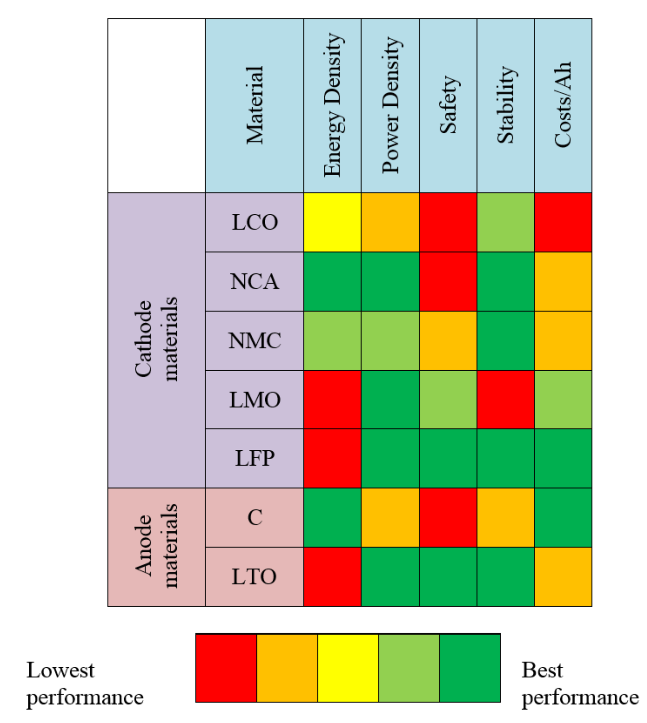
Traction batteries need characteristics such as high energy density and power density. The Ragone plot [5] shows that, among the established technologies, lithium-ion and lithium-polymer cells are those that best satisfy these requirements. Other advantages addressable to Li-ion batteries are the high cell potential and the high charge/discharge rate [6,7]. However, there are still some drawbacks mainly related with cost, safety, cycle life and lithium reliability. Further distinctions must be introduced within the lithium-ion batteries. According to [8], a first classification can be done based on the shape of the cell. A battery cell can be manufactured in different shapes, typically cylindrical, prismatic and pouch. Cylindrical cells have the lowest energy density compared to the others; however, they are the cheapest to be produced so they are still widely used also in the automotive field. Prismatic cells have higher energy density and are characterized by an external hard case. Pouch cells are flexible, and they can be produced in different formats and are characterized by the higher energy and power density. A second classification [6] can be made according to the materials present inside the battery. The main elements inside a battery are the anode, the cathode, the separator between the electrodes and the electrolyte. Nowadays, the active materials composing the battery electrodes are objects of lots of research studies [9]. The best compromise must be identified considering lots of factors such as terminal voltage, capacity, number of cycles, safety and cost. Typical materials employed for the anode are Graphite and more recently Lithium Titanate (LTO). Among the structures used in the cathodes, there are Lithium Cobalt Oxide (LCO), Lithium Manganese Oxide (LMO), Nickel Manganese Cobalt Oxide (NMC), Nickel Cobalt Aluminium Oxide (NCA) and Lithium Iron Phosphate (LFP) [6]. Figure 1 summarizes the main performance of these electrode materials. Many combinations of anode and cathode materials can be used. Among the commercialized cells, a dominant position is awarded by the LFP-Graphite (LFP/C) batteries, which guarantee the best results in terms of both safety and lifetime. With respect to other chemistries, LFP is less prone to thermal runaway. This phenomenon leads to a chain of unstoppable exothermic reactions. The high amount of heat generated leads to the release of flammable and toxic gasses and sometimes to fire and explosions [10,11].
In the last few years, the need to study batteries in real working conditions has increased the demand for high specific testing equipment. Regarding programmable devices able to charge and discharge battery cells, there are two main solutions on the market. The first and more expensive one consists of an integrated device able to perform both tasks. This device is often multi-channel equipment that at the same time is able to handle many cells. It is also provided with a proprietary software that allows performing more or less personalized testing profiles. The second solution, usually pursued when a small number of cells must be tested, consists of dedicating a device to the charging stage and one to the discharging stage, respectively a power supply and an electronic load. Sometimes, a proprietary software can be provided by the manufacturers of the two devices to remotely control them; however, also in this case, the possible profiles are limited. Further attention must be paid to their integration. For example, if a profile contains both charging and discharging stages, the control software at the same time should be able to give proper commands to the devices. In the literature, some works in which the main focus is put on the system architecture design and the software development can be found [4,12]. Thus, because of economic reasons and in order to build flexible equipment to test battery cells, in this work, the testing layout is defined using two different programmable power units and a control platform was implemented in the NI LabVIEW environment (NI LabVIEW 2016, National Instruments, Austin, TX, USA). The platform consists of a software/hardware interface deployed on a real-time target PC. It is designed as a state machine structure and allows several testing modes.
In the following sections, the acquired data are elaborated to implement a state of charge estimation algorithm. Since computational capabilities on a BMS are limited, among the models presented in the literature [13,14], the authors decided to implement a simple but effective model without the claim to establish a new modelling technique. Among the most used algorithms in vehicles’ applications, there are adaptive techniques. These techniques can lean on different battery models [15]. The most used battery models are the Equivalent Circuit Models (ECMs) because they are quite intuitive, they are characterized by a reduced number of parameters and need a low computational effort with respect to the required accuracy [16]. These models represent battery cells by using electric components such as voltage generators, resistors and capacitors. These models representing a single cell can also be used to simulate more cells connected together [17,18]. In the present work, two different equivalent circuit models are investigated that are the Rint model and the Dual Polarization (DP) model. Thus, according to these ECMs, the battery is modelled and the parameters identification procedure is carried out using different techniques. Finally, the model developed is exploited to implement the state of charge estimation based on a Kalman filter algorithm [19,20]. The results are thus presented and discussed.
2. Testing Equipment
Considering the growing diffusion of Battery Electric Vehicles (BEV), the need of deeper knowledge on battery performance has increased the demand for advanced testing activities. The main aim of these tests is to allow the Cell Under Test (CUT) to experience conditions similar or more stressful than the actual ones and to explore its long-term behaviour. Moreover, standard tests are defined to compare different types of batteries and to characterize them [21,22].
To investigate the main aspects of a cell behaviour in different loading conditions, battery testing systems are equipped with two main power units: an electronic load and a charging unit [23]. The former is a device able to apply a predefined load to a battery using one of the following control modes:
- Constant Current (CC) mode: the applied load is regulated to keep the sunk current equal to the defined value despite the cell voltage is varying.
- Constant Voltage (CV) mode: the load is controlled to keep its terminal voltage equal to the defined set-point.
- Constant Power (CP) mode: the load is regulated to match a defined power set-point; the sunk current is regulated in order to control the product Voltage per Current.
- Constant Resistance (CR) mode: the load is regulated to have a sunk current proportional to the applied voltage.
The latter is designed to apply a certain charging profile to the battery. Many studies are being conducted in the direction of reducing the battery charging time without impacts on the battery lifetime [24,25] also taking into account the effect of temperature [26]. The standard charging technique taken as comparison reference is the CC-CV technique suggested by cell manufacturers. This technique at the present stage guarantees better performance in terms of capacity retention; however, it requires long charging time. The CC-CV technique consists of two main charging steps: a Constant Current (CC) step where a current between 0.5–1 C is applied until a voltage upper threshold is reached; a Constant Voltage (CV) step where the current is regulated to keep the cell voltage equal to the reached threshold as shown in Figure 2. The charging procedure stops when the end-of-charge current is reached. The quantity C represents the amount of constant current that is necessary to fully discharge a cell in one hour and is numerically equal to the cell capacity expressed in Ampere per hours.
The combined use of these two devices allows for applying different user defined charging/discharging profiles to meet the need to study the battery behaviour in specific working conditions. Battery testing system manufacturers provide equipment with integrated multi-channel charging/discharging units, managed with dedicated proprietary software [27].
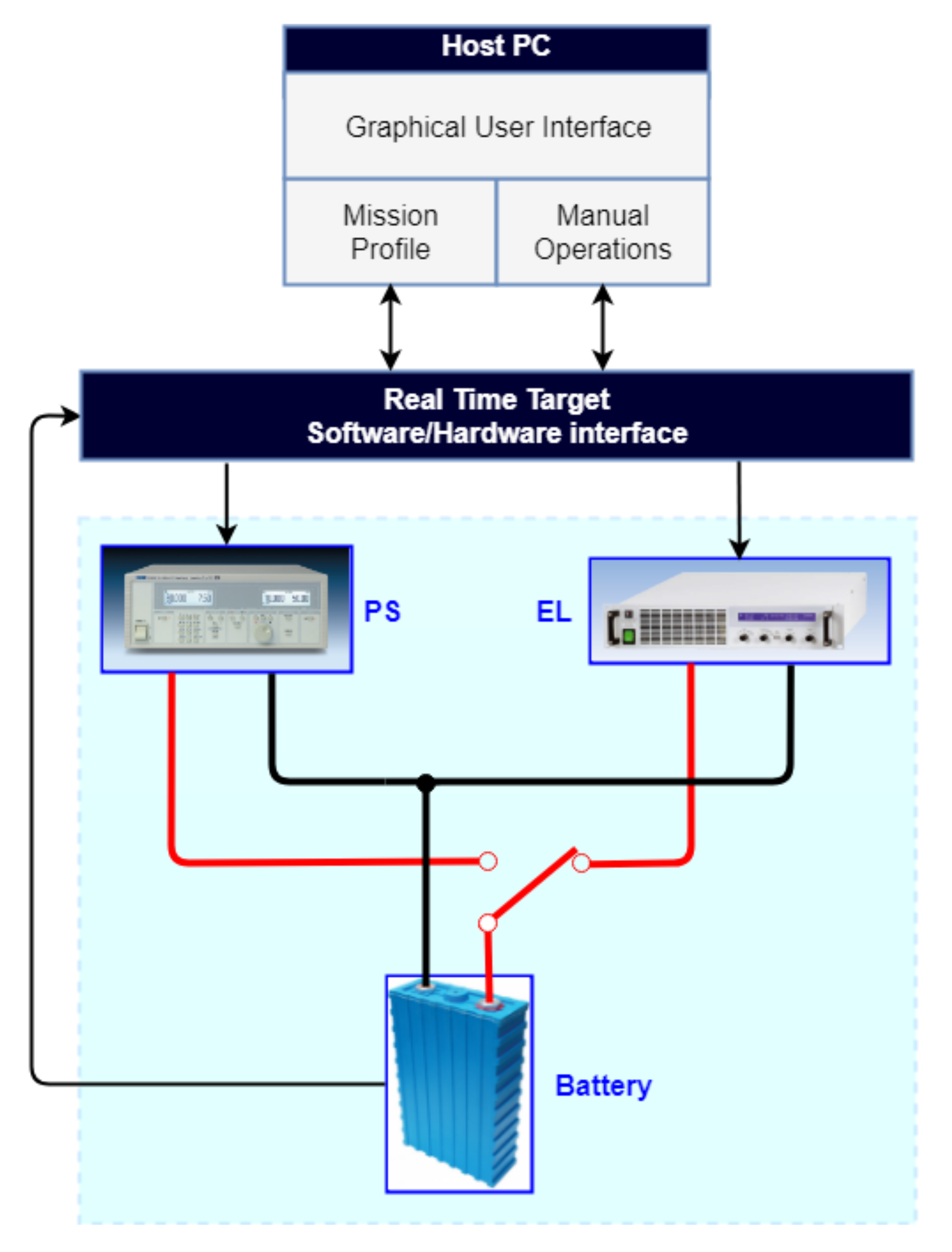
In this work, the testing layout was built using an EA-EL 9080-400 electronic load from Elektro-Automatik (Viersen, Germany), deputed to the discharging phase of the CUT, and a QPX-600DP power supply from Aim TTi (Huntingdon, United Kingdom), for feeding energy into the cell with a CC-CV logic. The resulting system layout is shown in Figure 3. The CUT key specifications are summarized in Table 1.
The two power units are controlled through a multifunction I/O module (NI PXIe 6363) from National Instruments (Austin, TX, USA). A software/hardware interface was developed within the NI LabVIEW environment and deployed on a Real Time controller (NI PXIe 8840). The user can interact with the system thanks to a Graphical User Interface (GUI) running on a Host Personal Computer. The NI PXIe 8840 is also devoted to the data acquisition. The voltage on the cell tabs is measured using a four-terminal sensing; the current flowing is provided by the two devices and is communicated to the Data Acquisition (DAQ) system through the analogue interfaces. Finally, during the tests, the cell temperature was continuously acquired in order to check that it was within the safety range; otherwise, everything is stopped.
Software-Hardware Interface Design
The considered power units are provided with embedded dedicated hardware control sections, so the software/hardware interface running on the controller must manage the following aspects:
- allow for manual or automatic settings;
- import user defined load profile through data tables;
- elaborate data to have useful signals for the power units;
- execute safety protocols;
- assign controls within determined timed intervals;
- read measurements and save data on a log file.
These top-level functions were implemented within the LabVIEW environment with a Producer–Consumer design pattern. Two main while loops run in parallel with different rates and execution priority. The first one is the Producer Loop (PL) shown in Figure 4.
The PL has the top execution priority since it must run on the controller with deterministic time intervals. The determinism of this loop is essential when it comes to safety shutdown procedures. A dedicated module is designated to evaluate if control variables and feedback measurements define a safe operating point for the cell. If not, an emergency shutdown procedure is immediately executed. Two other important functions are implemented inside this loop. After the approval of the Safety Control Unit (SCU), the set point values for both the electronic load and the power supply are defined and assigned through the output Digital to Analog Converter of the NI PXIe 6363 module. Moreover, data acquired through the Analog to Digital Converter of the same multifunction module are organized and sent to a queue that will be managed by the Consumer Loop (CL) shown in Figure 5.
The CL must continuously read data from the queue to empty the dedicated memory and to allow further PL writings. The PL runs with a sampling period of 250 ms; however, since this sampling rate is excessively fast for the CL, taking into account the sampling requirements needed for the specific user defined profile, a proper under-sampling algorithm was developed to have smaller log file dimensions. Finally, a user-friendly GUI was developed (Figure 6). It runs on a Host PC, allowing the user to:
- upload a predefined load history;
- define how many times the cycle must be repeated;
- define the number of cycles to be executed;
- have the main feedback measurements always available;
- stop the running tests whenever needed.
3. Battery Modelling
The devices and the experimental setup presented in the previous sections are fundamental to perform battery testing. Nowadays, we are interested in discovering the actual batteries’ potentiality. In fact, battery datasheets are still too poor in providing useful information for vehicles’ applications. A common battery datasheet contains fundamental information such as the battery chemistry, dimensions, capacity, internal impedance, nominal voltage, end-of charge voltage and current, end-of-discharge voltage, charging specifications in terms of maximum current in CC mode, maximum continuous and pulsed discharge current, cycle life, operating temperature range together with the typical discharging curves. However, this information refers to standard tests performed by the manufacturers, obtained from static tests that are not representative of actual working conditions. The main aim of these data is to define the battery Safety Operating Area (SOA) that determines the combination of the different quantities, which allow the battery to operate in safety conditions [13]. These data are not sufficient in vehicles’ applications where it is important not only to work safely, but also to guarantee certain performance. Additional information that is very interesting to a battery user is, for example, the cycle life in actual duty cycles and the actual capacity according to the discharging strategy; thus, it is necessary to further test batteries. Finally, abuse tests have great importance too because they allow for simulating in controlled environment the consequences of dangerous events and they can help provide the guidelines for the design of safety precautions. Common abuse tests are thermal runaway, short circuits and mechanical stress [28,29,30], and they are often followed by post-mortem analysis [31].
A battery pack must provide power to the electric motor, so it is fundamental to guarantee a certain voltage requirement. Depending on the electrified architecture considered, the required voltage is 12 V for micro hybrid vehicles, 48 V for mild hybrid vehicles, and going up to more than 600 V for high power applications [32,33,34].
In this work, a Li-ion Energy Storage System (ESS) is considered and the attention is focused on a single cell. A Li-ion battery pack must be equipped with control electronics, called Battery Management System (BMS), with the aim of handling the single cells allowing them to remain in their SOAs. The BMS also communicates with the vehicle control unit to which it provides information about the current battery state. Among this information, there is the estimate residual capacity inside the battery pack. This information is very important because it influences the vehicle control unit energy management strategy [35]. We can imagine the battery pack as a fuel tank where the fuel is represented by the current. When the user crushes the pedal, the required amount of power flows outside each single cell of the battery pack. Thus, to compute the battery used capacity, it is possible to simply compute the amount of current flown outside the battery according to the well-known Coulomb Counting technique, considering the uncertainties connected to the current measurements. A first difficulty grows when considering multiple cells that, because of the manufacturing process, do not have the same behaviour [36,37,38]. The residual capacity they store and the amount of current they deliver is not the same, and the battery capacity stored level is defined by the weakest cell. In this work, we are just considering a single cell, so we can overcome this drawback. However, if it is relatively simple to compute the cell used capacity, is it not the same if we consider the residual capacity, which is defined as the difference between the total available capacity and the used capacity. In fact, we can imagine the cell as a variable volume tank where the total volume is mainly influenced by the amount of current demanded, the operating temperature and the battery ageing. This condition is amplified if we speak in terms of power because, when the battery is emptying, it provides a lower voltage. Many algorithms were developed and are currently under study to provide a value of residual capacity that is as precise as possible. These algorithms often refer to a dimensionless quantity that is the State Of Charge (SOC), defined in Equation (1) [14,39]. To consider the capacity reduction with temperature, current and number of cycles, different strategies can be implemented such as the definition of indices or Look Up Tables (LUTs) after proper tests [40,41]. Among the most used indices, there are the State of Health (SOH) [42], the State Of Energy (SOE), the State Of Power (SOP), the State Of Function (SOF) and the State Of Safety (SOS) [43,44,45]:
In Equation (1), Qavailable is the available capacity, which mainly varies with the current rate, temperature and ageing. The used capacity Qused can be simply computed integrating the current in a certain time interval.
Among the most used algorithms for vehicles’ applications, there are the adaptive techniques. These techniques can lean on different battery models [15]. The most used battery models are the Equivalent Circuit Models (ECMs) because they are quite intuitive, they are characterized by a reduced number of parameters and need low computational effort with respect to the accuracy [16]. These models represent battery cells by using electric components such as voltage generators, resistors and capacitors. These models represent a single cell; however, they can also be used to simulate more cells connected together [17,18].
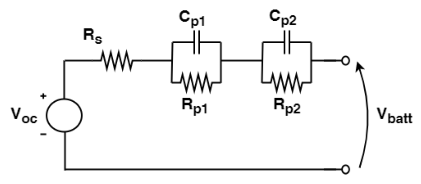
In the present work, two different equivalent circuit models are investigated. The simplest ECM is the Rint model, where the cell is represented as a voltage generator and a series resistor. The voltage generator represents the battery Open Circuit Voltage (VOC), which is the voltage at the battery terminals when no load is applied, and all the transients are extinguished. The series resistor represents the battery internal impedance that produces a voltage drop when some current flows through the battery. A Dual Polarization (DP) model is considered too in comparison to the previous one. This model is obtained from the previous one by adding, in series with the other electric components, two Resistor-Capacitor (RC)-branches whose aim is that of representing the battery transient behaviour due to the polarization. In fact, the battery transient voltage can be fitted by a function that is the sum of exponential functions with different time constants. As widely documented in the literature, a good compromise between accuracy and computational effort is obtained when two time constants, corresponding to the two RC branches, are considered [46]. However, attention must be paid in the selection of the transient period, as it will be discussed in more detail in the next sections. The described models can be summarized by means of Equations (2) and (3), respectively, for the Rint model and the DP model, while the schematic representation in shown in Figure 7. The current is assumed to be positive for discharging and negative for charging:
In these models, resistors and capacitors are modelled as constant parameters. The SOC dependency was not taken into account in these parameters because in vehicles’ applications the battery is mainly used in the range 20%–80% SOC, where the SOC dependency on these ECMs parameters is not too strong.
Vice versa, the open circuit voltage mainly varies according to the battery residual capacity so the VOC vs. SOC relationship is considered. This relationship can be implemented in different ways. In this work, two different kinds of functions are investigated, which are a polynomial function and an LUT. A more detailed description of this relationship is presented in the following section. Concerning other effects, such as temperature, hysteresis and ageing, their effect is not considered in the ECM. It is well known that temperature influences the battery electrical parameters and thus the battery performance too. However, because the cell was subjected to natural convection and the testing were not too aggressive, the temperature increase was restrained and its effect was not taken into account.
Open Circuit Voltage Modelling
Many different models were developed to represent the open circuit voltage behaviour with respect to the SOC. Among these, the simplified electrochemical models are widely used [47]. These models describe the battery voltage behaviour by means of some coefficients that have not a physical meaning; however, they allow a good fitting on the voltage curve. In this work, a Combined model is used, which is given by the collection of the Shepherd model, the Unnewehr universal model and the Nernst model. The model is expressed by Equation (4); to simplify the notation, the SOC is indicated as z. This model shows singularities in SOC=0 and SOC=1, so its value is limited within this range:
where k indicates the k-th sample with , …, N and N = number of samples. Instead of being constrained by a polynomial expression describing the whole curve trend, another way to express the relationship between VOC and SOC is to use a LUT. The LUT is a piecewise-linear, or higher order, function.
4. Model Parameters’ Identification Procedure
In this section, battery model parameters appointed previously are identified. Different parameters’ identification techniques can be applied.
4.1. Voltage Drop Based Parameters’ Identification
Concerning the identification of the VOC LUT and of the other ECM parameters, a parameters’ identification procedure based on the battery terminal voltage drops is implemented. As explained previously, when no load is applied, the battery terminal voltage is the open circuit voltage. When a load is applied, a voltage drop occurs. The voltage drop can be distinguished in an instantaneous voltage drop and a transient voltage drop. The instantaneous voltage drop can be exploited to identify the series resistor model parameter, while the transient behaviour can be exploited to identify the RC branches’ model parameters. To fulfill this target, a pulsed discharging profile is applied. In Figure 8, it is possible to see a portion of the pulsed discharge from which the parameters where identified. It is fundamental to select a proper pulse duration that is significant of actual pulse profiles because the time constant of the transient will vary according to the time interval considered. In fact, if a function given by the sum of two exponentials is used to fit a transient period of different durations, the resulting time constants are not the same. The authors decided to select a time interval to be fitted of 60 s as significant for vehicles’ applications. Thus, the battery terminal voltage between the instantaneous voltage drop and a 60 s time interval was fitted with a two time constants’ exponential function. The results are summarized in Table 2, where τp = Rp · Cp .
Finally, a pulsed discharging profile together with a pulsed charging profile can be exploited to identify the VOC LUT [48]. When a discharge pulse is applied and removed, the battery terminal voltage tends to return to its stationary value (that corresponds to the open circuit voltage); however, it requires a long time (more than 10 hours [49]) to fully reach this value. If a lower time interval is considered, the terminal voltage remains below this value. Similarly, if a charge pulse is applied and removed, the battery terminal voltage remains over the stationary value. The longer the rest period is, the closer is the distance between the upper and the lower limit [50]. Thus, a certain number of discharge and charging pulses, for various values of SOC, can be taken into account. The envelope of the upper points of the discharging curve and the envelope of the lower points of the charging curve can be considered. These points define the upper and the lower VOC bounds; therefore, the VOC vs. SOC relationship can be determined by computing the mean values among these bounds [51]. A representation of the result of the described procedure is presented in Figure 9 and a summary of some significant points is collected in Table 3. The VOC vs. SOC curve representation as a look up table is not dependent on the battery model implemented to simulate the battery terminal voltage. The VOC is present both in the Rint and in the DP model, so the LUT relationship identified can be used in both models.
4.2. Least Squares Procedure Parameters’ Identification
If we consider the Rint model with an open circuit voltage described by a Combined model, summarized in Equation (5), an easier and faster way to identify the model parameters can be implemented through the Least Squares Procedure (LSP):
Once the parameters to be identified are defined (Equation (6)), the coefficient matrix A (Equation (7)) and the output vector Y (Equation (8)) are computed [52]:
where N is the number of samples. The LSP solution is given by Equation (9), which provides the identified model parameters :
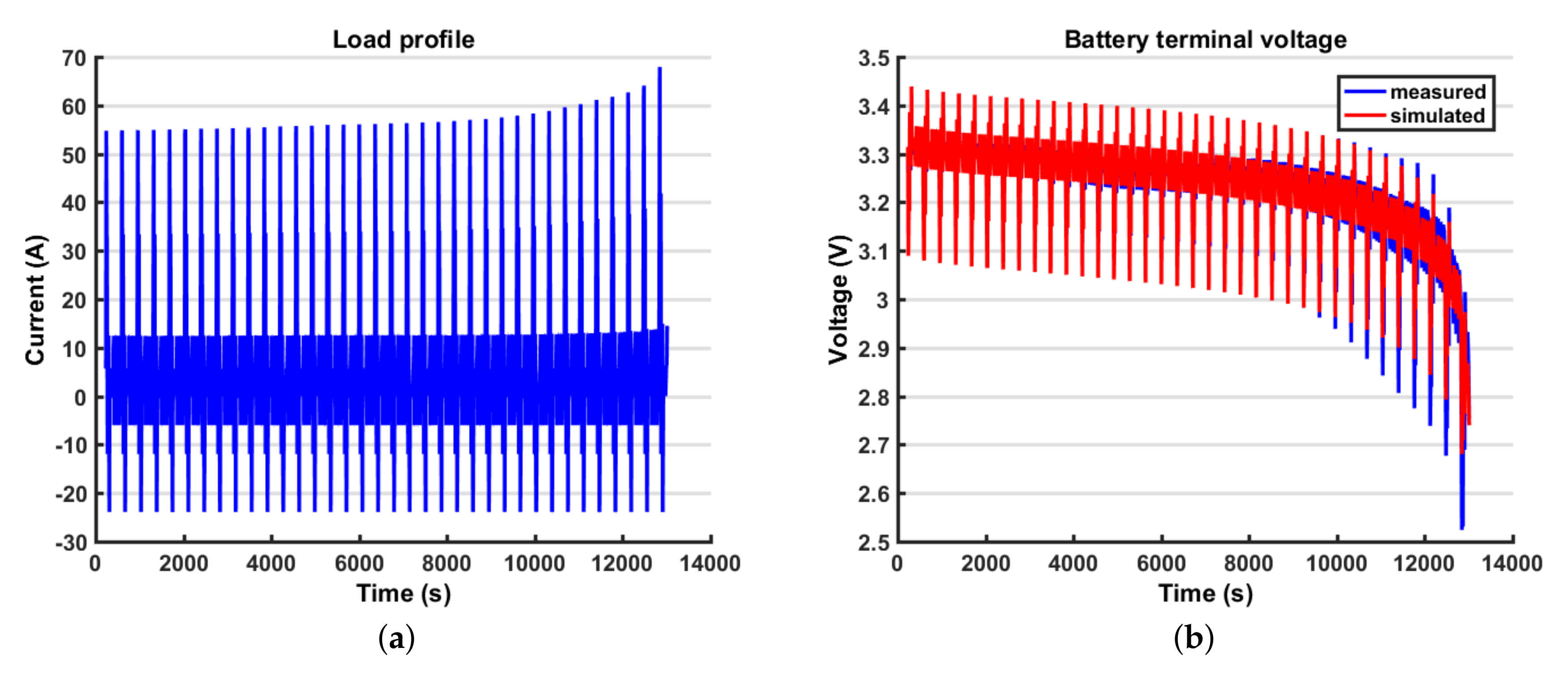
A standard Dynamic Stress Test (DST) profile was applied to identify the parameters because it guarantees a low conditioning number of the coefficient matrix. The DST was designed by the USABC (US Advanced Battery Consortium) to represent the dynamic EV working profile [21]. It consists of a series of positive and negative impulses of different duration, the amplitude and the duration of which are defined by the standards. The single cycle duration is 360 s, and it is repeated until the cut off voltage is reached. The standard cycle is presented in terms of percentage of the discharge power. Once the maximum allowed constant discharging current is fixed, the 100% amplitude of the profile corresponds to the 80% of the power delivered by the battery at 20% SOC. The test was performed in ambient temperature at 20 °C because, when the battery is at a low charge, the terminal voltage decreases in order to guarantee the same amount of power the delivered current increases, as shown in Figure 10a. Figure 10b shows the measured data overlapped to the simulated output. The model follows the discharging macroscopic trend, but it is not able to catch the transient behaviour. The values of the identified parameters are summarized in Table 4.
The same procedure was applied to the VOC data obtained from the pulsed charge/discharge to compare the results. Obviously, the parameters are different because the data from which they were identified are different. Furthermore, when fitting the DST output curve, a part of the voltage drop is included in the contribution of the term R0.
Because the VOC was identified in two different ways, it is possible to validate estimation procedures by comparing the results from the two methodologies. In Figure 11a, it is possible to notice that the piecewise-linear function is able to better describe the voltage behaviour because it is not limited by the necessity to be fitted by a polynomial in the whole SOC variation range. Furthermore, in the Combined Model, the load profile is mainly a discharging profile, and this is the reason why the Combined Model VOC curve is below the LUT identified curve. The LUT curve is also able to describe the initial exponential trend of the VOC curve. However, the overall trend is similar.
5. State of Charge Estimation
In this section, the state of charge estimation algorithm implemented is described. As outlined previously, an adaptive method was implemented for the state of charge estimation. We must talk about estimation because, from this technique, we can only obtain an estimation of the searched value. The authors’ choice fall on the Kalman Filter (KF) technique, which is widely adopted in this field [53].
Extended Kalman Filter Algorithm
The Kalman Filter consists of defining a certain number of inputs u, outputs y and states x. The inputs and the outputs are known values, while the states are quantities the user is interested in, which cannot be measured. However, because the outputs depend on the states, it is possible to compute the errors between the actual outputs and the estimated outputs, which depend on the states errors. Thus, the states estimations can be corrected. Because the battery model selected is nonlinear, an Extended Kalman Filter (EKF) must be implemented. We can write the model in the state space (Equation (10)):
The bold font is used to indicate a non-scalar quantity. is the input vector, is the output vector and is the state vector; (…) is the state function, (…) is the measurement function; and , respectively, are the process noise and the measurement noise, and they are Gaussian noises with zero-mean and, respectively, covariances Qk and Rk. Thus:
It is possible to summarize the EKF technique in the following steps:
- Initialization (to be executed only once)
- Prediction step:A priori state estimationA priori error covariance matrix
- Correction step:Kalman gainEstimated outputPrediction errorA posteriori state estimationA posteriori error covariance matrixInnovation covariance matrixProcess noise covariance matrix updatewhere M is the number of samples of the moving estimation window. Zk is computed by the states errors and it allows to correct the covariance matrix Qk. Jf and Jh, respectively, are the Jacobian matrices of the model function and the output function, and they are shown in Equations (24) and (25):
The superscript indicates a a priori estimate, while the superscript indicates a a posteriori estimate. Pk is the error covariance. The matrices Qk and Rk must be set by the user. A low value of Qk means a high confidence in the model, and a low value of Rk means a high confidence in the measurement data. If the ratio Rk/Qk is high, the model convergence will be rapid with high fluctuations; vice versa, if the ratio Rk/Qk is low, the model convergence will be slow with low fluctuations. Because the measurements were conducted in the laboratory and it is known that the model is a simplification of the actual battery, a high ratio Rk/Qk was selected by the authors. The R value depends on the measurement and its value is set according to the instrumentation accuracy, so it was set to 10. The Q depends on the model accuracy. Due to the difficulties in evaluating this parameter, a first value of 5 was set. Then, an adaptive step is implemented in which the value of the noise covariance matrix is updated each time step in order to properly correct this value according to the data. It is important to set a proper value of Rk and Qk to let the algorithm work properly. In the present case, the model input and output are presented in Equations (26) and (27):
Concerning the state vector, for the Rint and the DP model, respectively, can be expressed by Equations (28) and (29):
The state space models are defined in Equations (32) and (33), respectively, for the Rint and the DP model:
where the term must be computed in z = zk-1, and, according to the Combined model, is defined in Equation (34):
When solving the EKF, it is necessary to check if the model states are observable. It is possible to express the Observability matrix by using Equation (35):
where A = Jf and C = Jh. We know from linear algebra that the system of linear algebraic equations with n unknowns has a unique solution if and only if the system matrix has rank n. Thus, the model is observable if Ob has full rank n. In MATLAB (MATLAB R2017b, MathWorks, Natick, MA, USA), we use the function obsv to check the system observability. We must always check that the number of unobservable states is zero.
6. Model Performance
It is possible to compute some statistical indices to perform a quantitative analysis of the comprehensive performance of the two models. The indices are computed both for the model output and for the estimated SOC: the former is compared with the measured voltage and the latter is compared with the theoretical SOC computed according to the Coulomb Counting technique.
7. Results
The results of the different models are presented and compared here. Figure 12, Figure 13 and Figure 14 show the results of the DST profile. The maximum temperature increase found in the test is 4.7 °C.
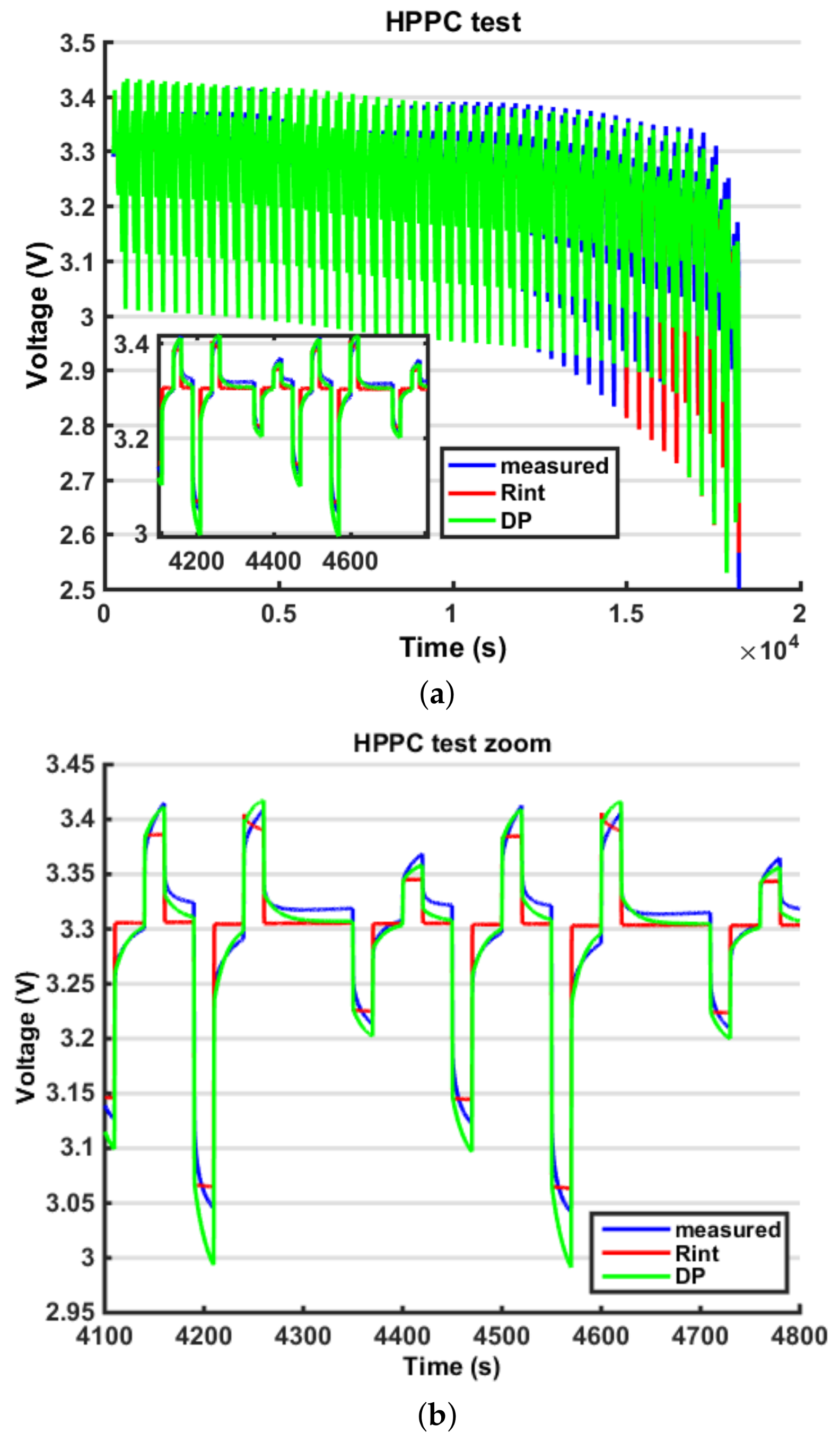
To further validate the model, a modified version of the Hybrid Pulse Power Characterization (HPPC) test was performed, and the current profile is shown in Figure 15. It consists of a series of positive and negative constant current pulses of growing amplitude, where the discharging current is 1C, 2C and 3C and the charging current is always a half of the discharging current. The duration of each pulse is 20 s and the pulses are separated by 30 s pauses; the last pause is 60 s. The total cycle duration is 360 s. This cycle is repeated in time until the cell cut-off voltage is reached. The results are shown in Figure 16, Figure 17 and Figure 18. The maximum temperature increase found in the test is 6.8 °C.
8. Discussion
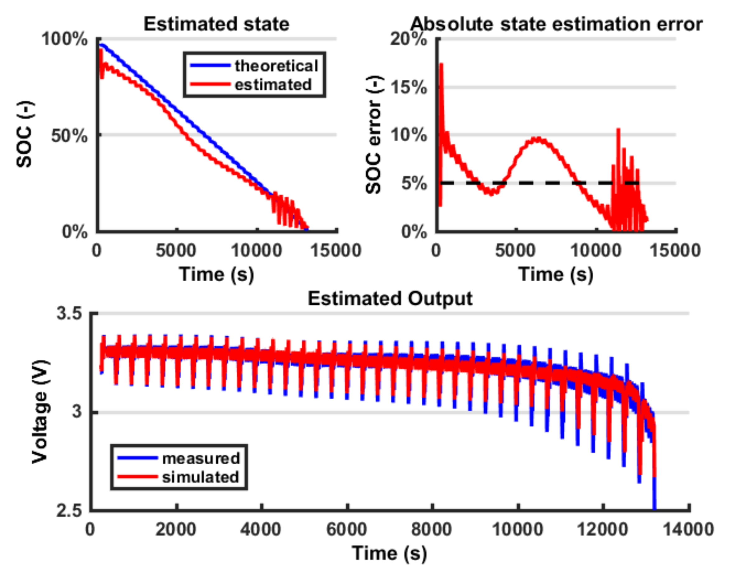
It is possible to notice that using a Combined Model for the VOC, moving from a Rint model (Figure 12) to a DP model (Figure 13), the estimated output fits the measured output better (Figure 14). A certain amount of error persists in both models because the battery model is not able to fully describe the battery behaviour; however, this error is within the 5% bound so it is considered acceptable. The outputs in terms of voltage are very similar; however, because of the EKF logic, the error on the output is compensated by a change in the state estimation, so the fluctuations found in the state estimation are connected to the error in the model. In the last part of the test, the state estimation error grows again because the model is less accurate; however, this interval is less significant because the battery is close to the prescribed cut-off voltage (below 20% SOC). Another difficulty in the output fitting can be found in the value of the battery impedance identification. In fact, because the parameters representing the resistance are modelled as constant with respect to the SOC, towards the end of the discharging process, the voltage drops can no longer fit the experimental data. The reason is that actually, when the SOC is low, the battery internal impedance grows, so a further improvement in the model would be to parametrize these coefficients with respect to the SOC. Finally, in Figure 18, it is possible to see how the DP model is able to fit the transient behaviour while the Rint model cannot. In conclusion, the major improvement from a Rint model to a DP model is on the output estimation error, which decreases, so it implies a better output simulation. However, this result does not always correspond to an improvement in the state estimation error. On the contrary, a simpler model such as the Rint model, is less subjected to fluctuations, so, in some cases, such as in the HPPC profile, it can produce lower errors on the state estimation error.
9. Conclusions
In this work, the possibility to build a platform that can act as an interface between the software and the hardware has been underlined. It is able to handle at the same time the charging stage and the discharging stage, imposing proper commands to the devices’ analogue interfaces. This platform is much more flexible than common proprietary software provided by the manufacturers. In the present work, this platform was exploited to apply used defined profiles while continuously checking that a cell’s voltage, current and temperature were within the safety ranges, and its functionality was proven. However, because of its structure, in which with a sampling period of 250 ms, input signals are given to the devices, this platform can be used for real-time simulations too. Further works will be developed to underline this task.
Author Contributions
E.V., F.M. and A.S. conceived and designed the experiments. E.V. and F.M. performed the experiments. E.V. analyzed the data.
Conflicts of Interest
The authors declare no conflict of interest.
References
- Chan, C.C. The State of the Art of Electric and Hybrid Vehicles. Proc. IEEE 2002, 90, 247–275. [Google Scholar] [CrossRef]
- Somà, A.; Bruzzese, F.; Mocera, F.; Viglietti, E. Hybridization factor and performance of hybrid electric telehandler vehicle. IEEE Trans. Ind. Appl. 2016, 52, 5130–5138. [Google Scholar] [CrossRef]
- Mocera, F.; Somà, A. Study of a Hardware-In-the-Loop bench for hybrid electric working vehicles simulation. Ecol. Veh. Renew. Energies (EVER) 2017, 1–8. [Google Scholar] [CrossRef]
- Barreras, J.V.; Fleischer, C.; Christensen, A.E.; Swierczynski, M.; Schaltz, E.; Andreasen, S.J.; Sauer, D.U. An Advanced HIL Simulation Battery Model for Battery Management System Testing. IEEE Trans. Ind. Appl. 2016, 52, 5086–5099. [Google Scholar] [CrossRef]
- Polleta, B.G.; Staffellband, I.; Shang, J.L. Current status of hybrid, battery and fuel cell electric vehicles: From electrochemistry to market prospects. Electrochim. Acta 2012, 84, 235–249. [Google Scholar] [CrossRef]
- Nitta, N.; Wu, F.; Lee, J.T.; Yushin, G. Li-ion battery materials: Present and future. Mater. Today 2015, 18, 252–264. [Google Scholar] [CrossRef]
- Opitza, A.; Badamia, P.; Shena, L.; Vignaroobana, K.; Kannana, A.M. Can Li-Ion batteries be the panacea for automotive applications? Renew. Sustain. Energy Rev. 2017, 68, 685–692. [Google Scholar] [CrossRef]
- Mulder, G.; Omar, N.; Pauwels, S.; Meeus, M.; Leemans, F.; Verbrugge, B.; De Nijs, W.; Van den Bosschec, P.; Sixa, D.; Van Mierlo, J. Comparison of commercial battery cells in relation to material properties. Electrochim. Acta 2013, 87, 473–488. [Google Scholar] [CrossRef]
- Passerini, S.; Scrosati, B. Lithium and Lithium-Ion Batteries: Challenges and Prospects. Electrochem. Soc. Interface 2016, 25, 85–87. [Google Scholar] [CrossRef]
- Wang, Q.S.; Ping, P.; Zhao, X.J.; Chu, G.Q.; Sun, J.H.; Chen, C.H. Thermal runaway caused fire and explosion of lithium ion battery. J. Power Sources 2012, 208, 210–224. [Google Scholar] [CrossRef]
- Lopez, C.; Jeevarajan, J.; Mukherjee, P.P. Experimental Analysis of Thermal Runaway and Propagation in Lithium-Ion Battery Modules. J. Electrochem. Soc. 2015, 162, A1905–A1915. [Google Scholar] [CrossRef]
- Collet, A.; Crébier, J.-C.; Chureau, A. Multi-Cell Battery Emulator for Advanced Battery Management System Benchmarking. IEEE Int. Symp. Ind. Electron. 2011, 1093–1099. [Google Scholar] [CrossRef]
- Lu, L.; Han, X.; Li, J.; Hua, J.; Ouyang, M. A review on the key issues for lithium-ion battery management in electric vehicles. J. Power Sources 2013, 226, 272–288. [Google Scholar] [CrossRef]
- Chang, W.-Y. The State of Charge Estimating Methods for Battery: A Review. ISRN Appl. Math. 2013, 1–7. [Google Scholar] [CrossRef]
- Hu, X.; Li, S.; Peng, H. A comparative study of equivalent circuit models for Li-ion batteries. J. Power Sources 2012, 198, 359–367. [Google Scholar] [CrossRef]
- Zheng, Y.; Ouyang, M.; Han, X.; Lu, L.; Li, J. Investigating the error sources of the online state of charge estimation methods for lithium-ion batteries in electric vehicles. J. Power Sources 2018, 377, 161–188. [Google Scholar] [CrossRef]
- Wei, J.; Dong, G.; Chen, Z.; Kang, Y. System state estimation and optimal energy control framework for multicell lithium-ion battery system. Appl. Energy 2017, 187, 37–49. [Google Scholar] [CrossRef]
- Bruen, T.; Marco, J. Modelling and experimental evaluation of parallel connected lithium ion cells for an electric vehicle battery system. J. Power Sources 2016, 310, 91–101. [Google Scholar] [CrossRef]
- Plett, G. Extended Kalman filtering for battery management systems of LiPB-based HEV battery packs. Part 2. Modeling and identification. J. Power Sources 2004, 134, 252–261. [Google Scholar] [CrossRef]
- Plett, G. Extended Kalman filtering for battery management systems of LiPB-based HEV battery packs. Part 3. State and parameter estimation. J. Power Sources 2004, 134, 277–292. [Google Scholar] [CrossRef]
- Hunt, G. USABC Electric Vehicle Battery Test Procedures Manual; United States Department of Energy: Washington, DC, USA, 1996.
- FreedomCAR Battery Test Manual for Power-Assist Hybrid Electric Vehicles; DOE/ID-11069; National Engineering and Environmental Laboratory: Idaho Falls, ID, USA, 2013.
- Chaoui, H.; Mandalapu, S. Comparative Study of Online Open Circuit Voltage Estimation Techniques for State of Charge Estimation of Lithium-Ion Batteries. Batteries 2017, 3, 12. [Google Scholar] [CrossRef]
- Abdel-Monem, M.; Trad, K.; Omar, N.; Hegazy, O.; Van den Bossche, P.; Van Mierlo, J. Influence analysis of static and dynamic fast-charging current profiles on ageing performance of commercial lithium-ion batteries. Energy 2017, 120, 179–191. [Google Scholar] [CrossRef]
- Keil, P.; Jossen, A. Charging protocols for lithium-ion batteries and their impact on cycle life—An experimental study with different 18650 high-power cells. J. Energy Storage 2016, 6, 125–141. [Google Scholar] [CrossRef]
- Zhang, C.; Jiang, J.; Gao, Y.; Zhang, W.; Liu, Q.; Huc, X. Charging optimization in lithium-ion batteries based on temperature rise and charge time. Appl. Energy 2017, 194, 569–577. [Google Scholar] [CrossRef]
- Zheng, F.; Xing, Y.; Jiang, J.; Sun, B.; Kim, J.; Pecht, M. Influence of different open circuit voltage tests on state of charge online estimation for lithium-ion batteries. Appl. Energy 2016, 183, 513–525. [Google Scholar] [CrossRef]
- Nedjalkov, A.; Meyer, J.; Köhring, M.; Doering, A.; Angelmahr, M.; Dahle, S.; Sander, A.; Fischer, A.; Schade, W. Toxic Gas Emissions from Damaged Lithium Ion Batteries—Analysis and Safety Enhancement Solution. Batteries 2016, 2, 5. [Google Scholar] [CrossRef]
- Larsson, F.; Andersson, P.; Mellander, B.-E. Lithium-Ion Battery Aspects on Fires in Electrified Vehicles on the Basis of Experimental Abuse Tests. Batteries 2016, 2, 9. [Google Scholar] [CrossRef]
- Ruiz, V.; Pfrang, A.; Kriston, A.; Omar, N.; Van den Bossche, P.; Boon-Brett, L. A review of international abuse testing standards and regulations for lithium ion batteries in electric and hybrid electric vehicles. Renew. Sustain. Energy Rev. 2018, 81, 1427–1452. [Google Scholar] [CrossRef]
- Waldmann, T.; Quinn, J.B.; Richter, K.; Kasper, M.; Tost, A.; Klein, A.; Wohlfahrt-Mehrens, M. Electrochemical, Post-Mortem, and ARC Analysis of Li-Ion Cell Safety in Second-Life Applications. J. Electrochem. Soc. 2017, 164, A3154–A3162. [Google Scholar] [CrossRef]
- Wu, G.; Zhang, X.; Dongn, Z. Powertrain architectures of electrified vehicles: Review, classification and comparison. J. Frankl. Inst. 2015, 352, 425–448. [Google Scholar] [CrossRef]
- Bayindir, K.C.; Gözüküçük, M.A.; Teke, A. A comprehensive overview of hybrid electric vehicle: Powertrain configurations, powertrain control techniques and electronic control units. Energy Convers. Manag. 2011, 52, 1305–1313. [Google Scholar] [CrossRef]
- Karden, E.; Ploumen, S.; Fricke, B.; Miller, T.; Snyder, K. Energy storage devices for future hybrid electric vehicles. J. Power Sources 2007, 168, 2–11. [Google Scholar] [CrossRef]
- Hannan, M.A.; Lipu, M.S.H.; Hussain, A.; Mohamed, A. A review of lithium-ion battery state of charge estimation and management system in electric vehicle applications: Challenges and recommendations. Renew. Sustain. Energy Rev. 2017, 78, 834–854. [Google Scholar] [CrossRef]
- Orcioni, S.; Buccolini, L.; Ricci, A.; Conti, M. Lithium-ion Battery Electrothermal Model, Parameter Estimation, and Simulation Environment. Energies 2017, 10, 375. [Google Scholar] [CrossRef]
- Narayanaswamy, S.; Kauer, M.; Steinhorst, S.; Lukasiewycz, M.; Chakraborty, S. Modular Active Charge Balancing for Scalable Battery Packs. IEEE Trans.Very Large Scale Integr. (VLSI) Syst. 2017, 25, 974–987. [Google Scholar] [CrossRef]
- McCurlie, L.; Preindl, M.; Emadi, A. Fast Model Predictive Control for Redistributive Lithium-Ion Battery Balancing. IEEE Trans. Ind. Electron. 2017, 64, 1350–1357. [Google Scholar] [CrossRef]
- Li, Z.; Huang, J.; Yann Liaw, B.; Zhang, J. On state-of-charge determination for lithium-ion batteries. J. Power Sources 2017, 348, 281–301. [Google Scholar] [CrossRef]
- Yang, R.; Xiong, R.; He, H.; Mu, H.; Wang, C. A novel method on estimating the degradation and state of charge of lithium-ion batteries used for electrical vehicles. Appl. Energy 2017, 207, 336–345. [Google Scholar] [CrossRef]
- Stroe, D.-I.; Swierczynski, M.; Stroe, A.-I.; Knudsen Kær, S. Generalized Characterization Methodology for Performance Modelling of Lithium-Ion Batteries. Batteries 2016, 2, 37. [Google Scholar] [CrossRef]
- Berecibar, M.; Gandiaga, I.; Villarreal, I.; Omar, N.; Van Mierlo, J.; Van den Bossche, P. Critical review of state of health estimation methods of Li-ion batteries for real applications. Renew. Sustain. Energy Rev. 2016, 56, 572–587. [Google Scholar] [CrossRef]
- Farmann, A.; Waag, W.; Marongiu, A.; Uwe Sauer, D. Critical review of on-board capacity estimation techniques for lithium-ion batteries in electric and hybrid electric vehicles. J. Power Sources 2015, 281, 114–130. [Google Scholar] [CrossRef]
- Farmann, A.; Uwe Sauer, D. A comprehensive review of on-board State-of-Available-Power prediction techniques for lithium-ion batteries in electric vehicles. J. Power Sources 2016, 329, 123–137. [Google Scholar] [CrossRef]
- Cabrera-Castillo, E.; Niedermeier, F.; Jossen, A. Calculation of the state of safety (SOS) for lithium ion batteries. J. Power Sources 2016, 324, 509–520. [Google Scholar] [CrossRef]
- Lai, X.; Zheng, Y.; Sun, T. A comparative study of different equivalent circuit models for estimating state-of-charge of lithium-ion batteries. Electrochim. Acta 2018, 259, 566–577. [Google Scholar] [CrossRef]
- He, H.; Xiong, R.; Guo, H.; Li, S. Comparison study on the battery models used for the energy management of batteries in electric vehicles. Energy Convers. Manag. 2012, 64, 113–121. [Google Scholar] [CrossRef]
- Abu-Sharkh, S.; Doerffel, D. Rapid test and nonlinear model characterisation of solid-state lithium-ion batteries. J. Power Sources 2004, 130, 266–274. [Google Scholar] [CrossRef]
- Huria, T.; Ceraolo, M.; Gazzarri, J.; Jackey, R. Simplified Extended Kalman Filter Observer for SOC Estimation of Commercial Power-Oriented LFP Lithium Battery Cells. SAE Tech. Pap. 2013. [Google Scholar] [CrossRef]
- Li, A.; Pelissier, S.; Venet, P.; Gyan, P. Fast Characterization Method for Modeling Battery Relaxation Voltage. Batteries 2016, 2, 7. [Google Scholar] [CrossRef]
- Huria, T.; Ludovici, G.; Lutzemberger, G. State of charge estimation of high power lithium iron phosphate cells. J. Power Sources 2014, 249, 92–102. [Google Scholar] [CrossRef]
- Yang, F.; Xing, Y.; Wang, D.; Tsui, K.L. A comparative study of three model-based algorithms for estimating state-of-charge of lithium-ion batteries under a new combined dynamic loading profile. Appl. Energy 2016, 164, 387–399. [Google Scholar] [CrossRef]
- Hua, X.; Li, S.; Peng, H.; Sun, F. Robustness analysis of State-of-Charge estimation methods for two types of Li-ion batteries. J. Power Sources 2012, 217, 209–219. [Google Scholar] [CrossRef]
- Wang, Y.; Zhang, C.; Chen, Z. On-line battery state-of-charge estimation based on an integrated estimator. Appl. Energy 2017, 185, 2026–2032. [Google Scholar] [CrossRef]
- Xiong, R.; Gong, X.; Mi, C.C.; Sun, F. A robust state-of-charge estimator for multiple types of lithium-ion batteries using adaptive extended Kalman filter. J. Power Sources 2013, 243, 805–816. [Google Scholar] [CrossRef]
Figure 1.
Summary of the most common cathode and anode materials’ performance.

Figure 2.
CC-CV charging technique.
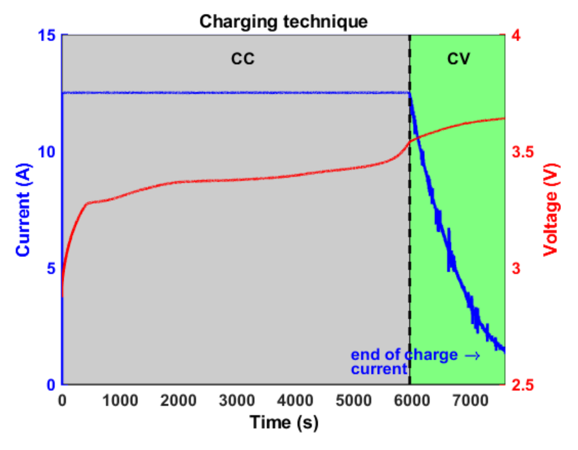
Figure 3.
Testing layout.

Figure 4.
Producer loop.
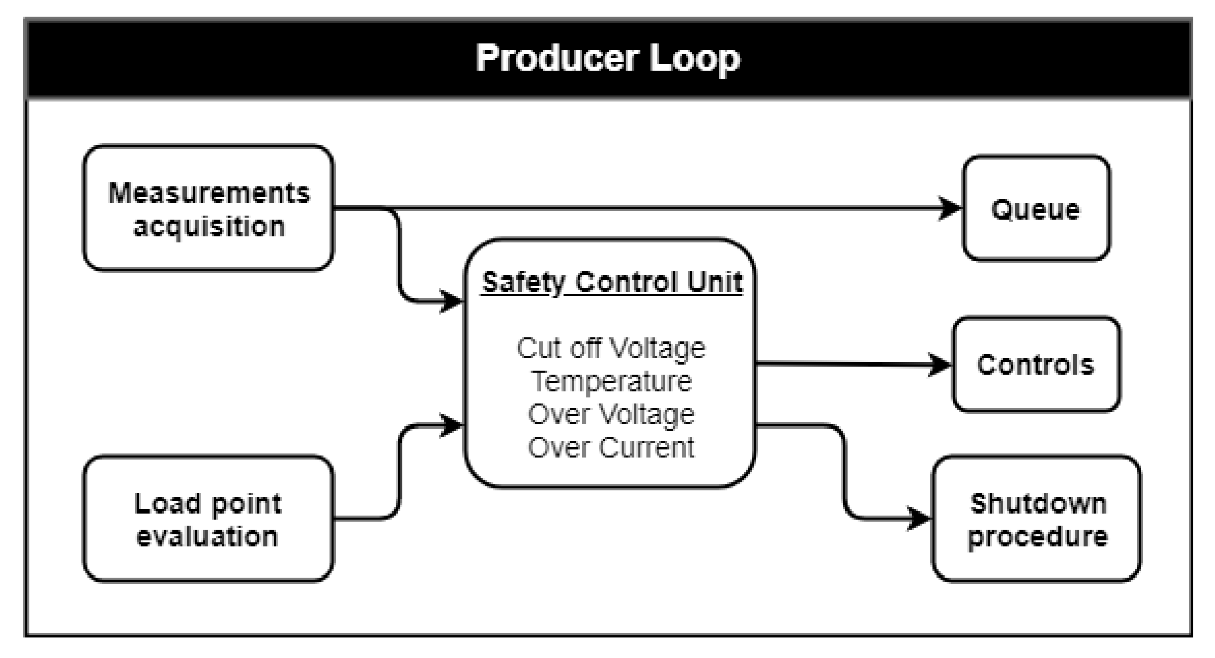
Figure 5.
Consumer loop.
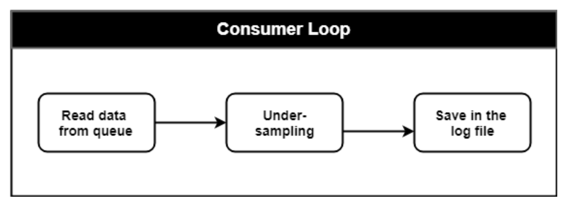
Figure 6.
NI LabVIEW Graphical User Interface.
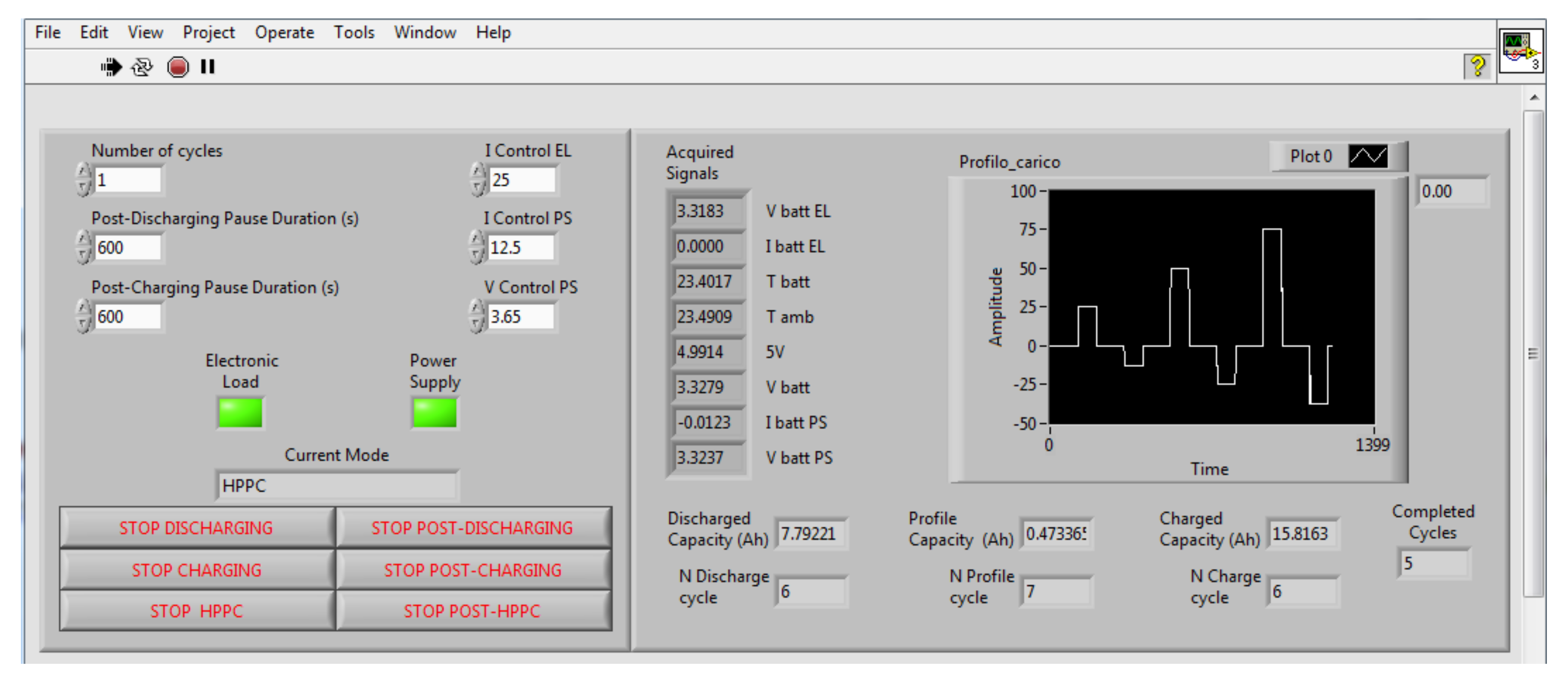
Figure 7.
Equivalent circuit model.

Figure 8.
Parameters’ identification from voltage drops.
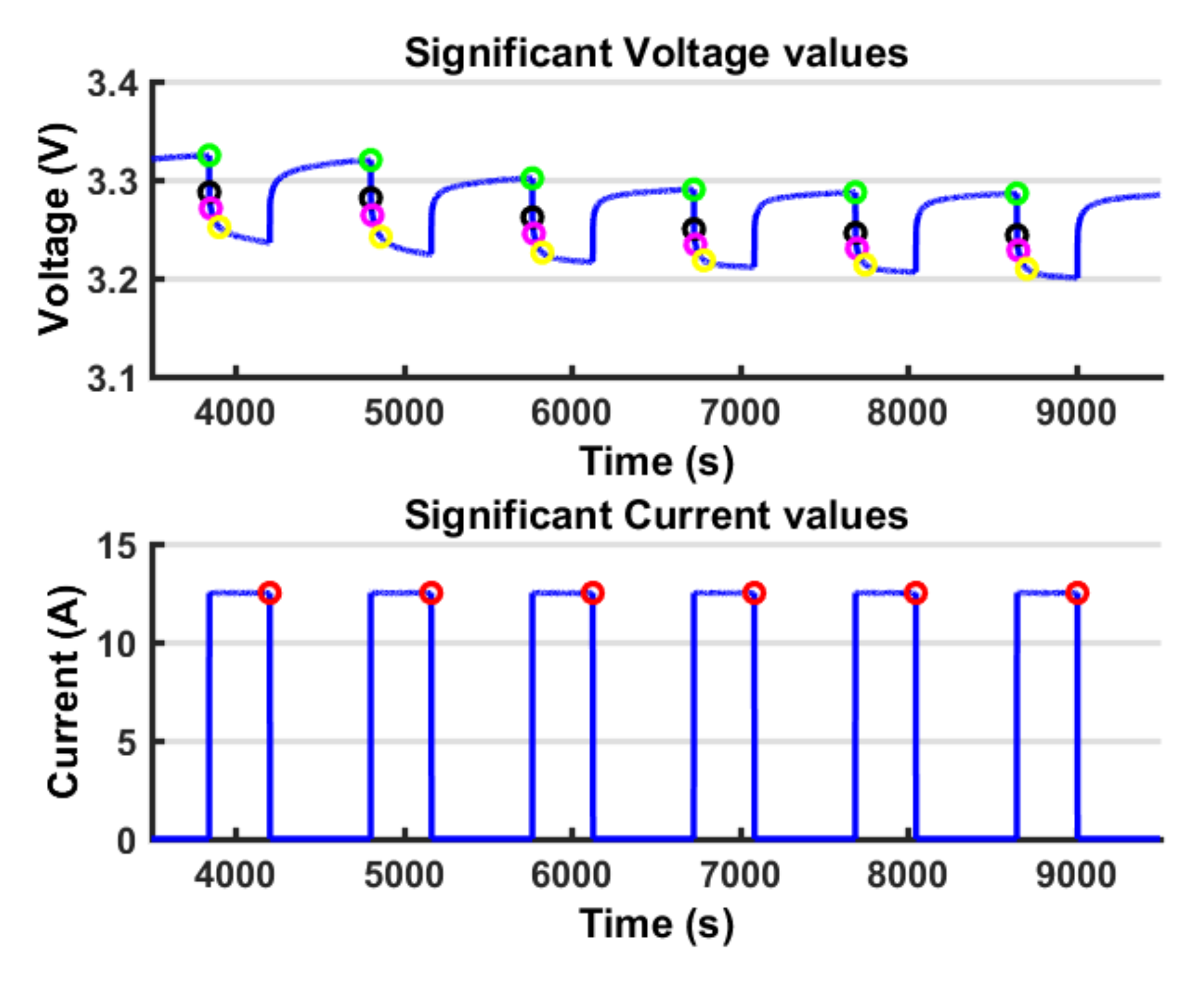
Figure 9.
VOC vs. SOC identified relationship by means of the pulsed charge and discharge profiles.
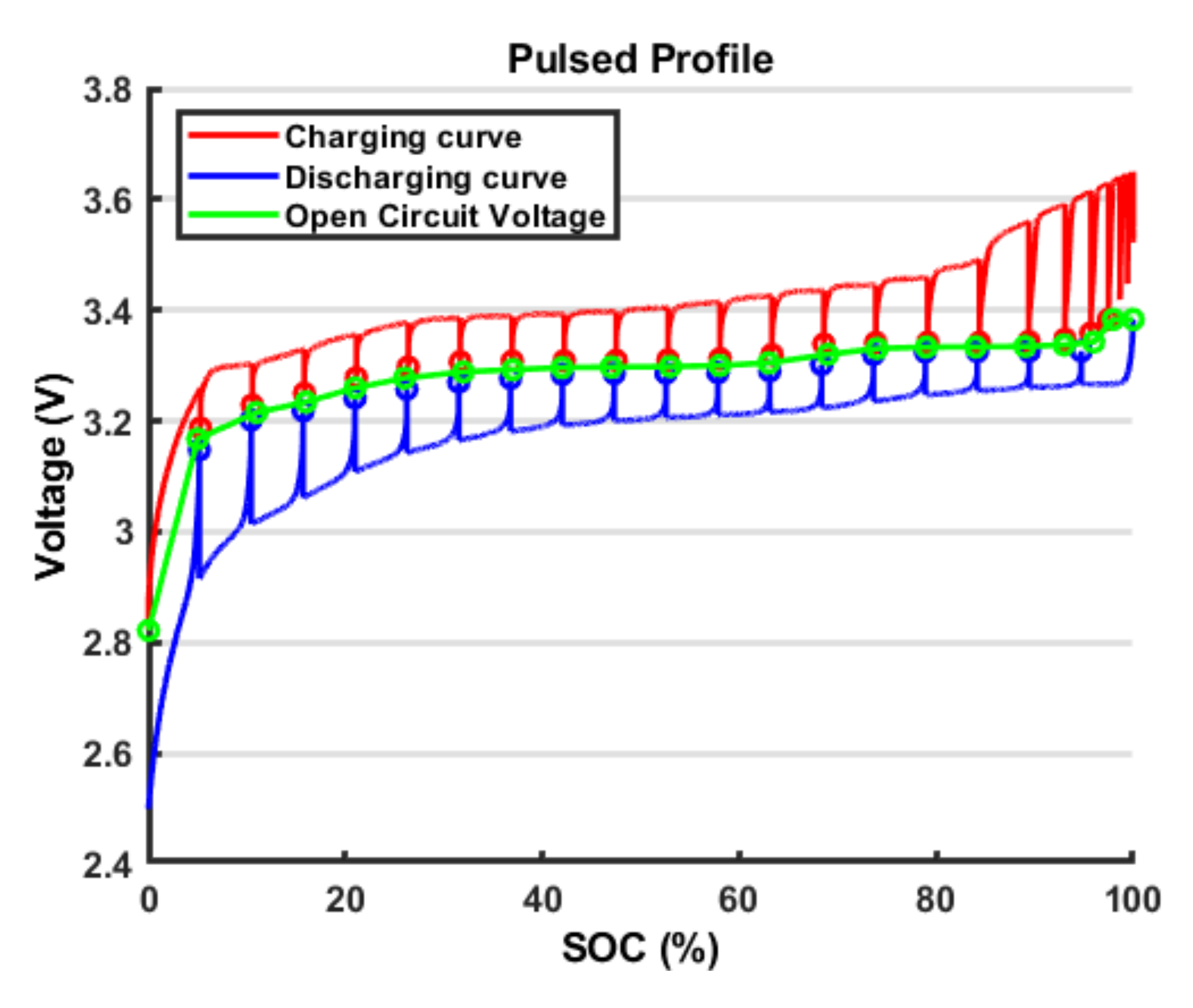
Figure 10.
Dynamic Stress Test (DST) profile voltage output. (a) current; (b) voltage.

Figure 11.
Open Circuit Voltage curve. (a) comparison between the VOC vs. SOC relationship identified according to the Combined model and to the LUT; (b) comparison between the VOC curves obtained from the Combined model parameters, respectively, from Table 4 and Table 5.
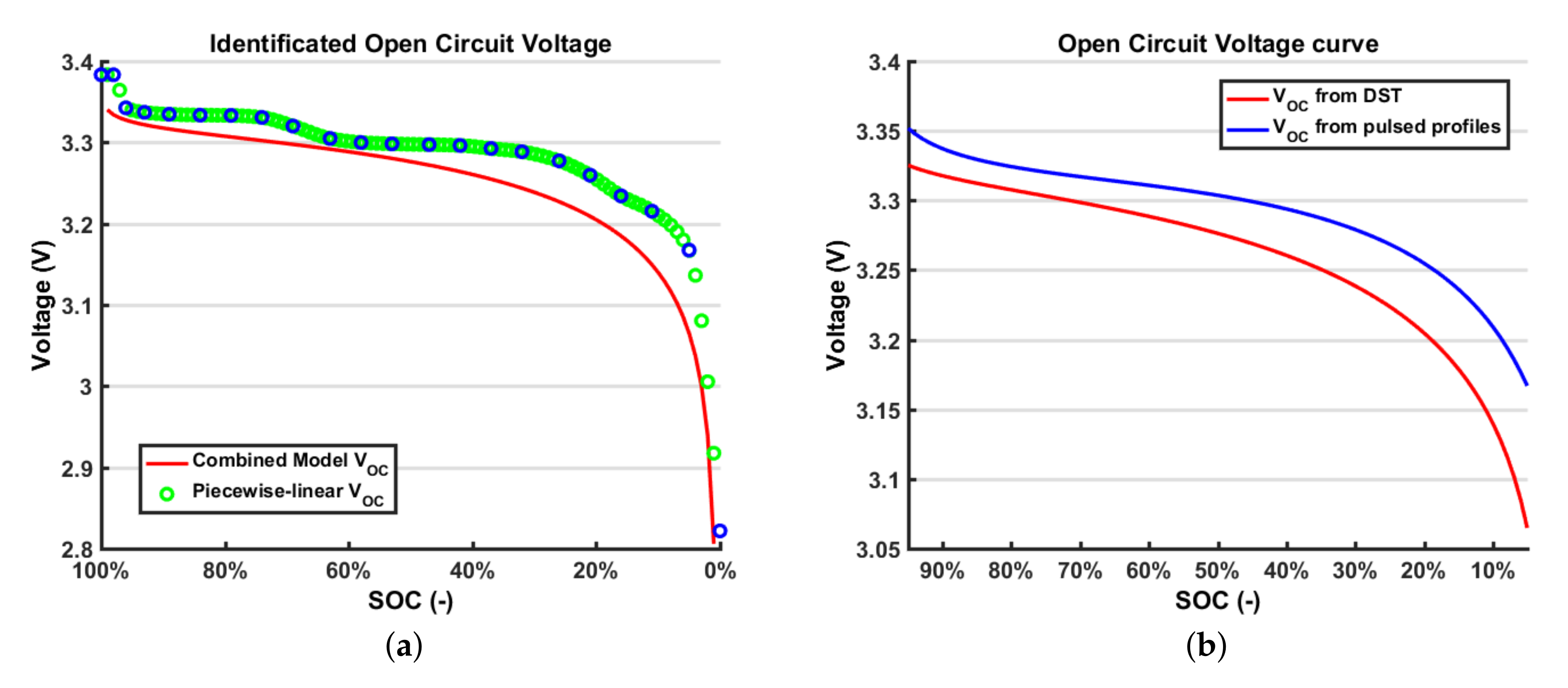
Figure 12.
Combined-Rint model.

Figure 13.
Combined-DP model.
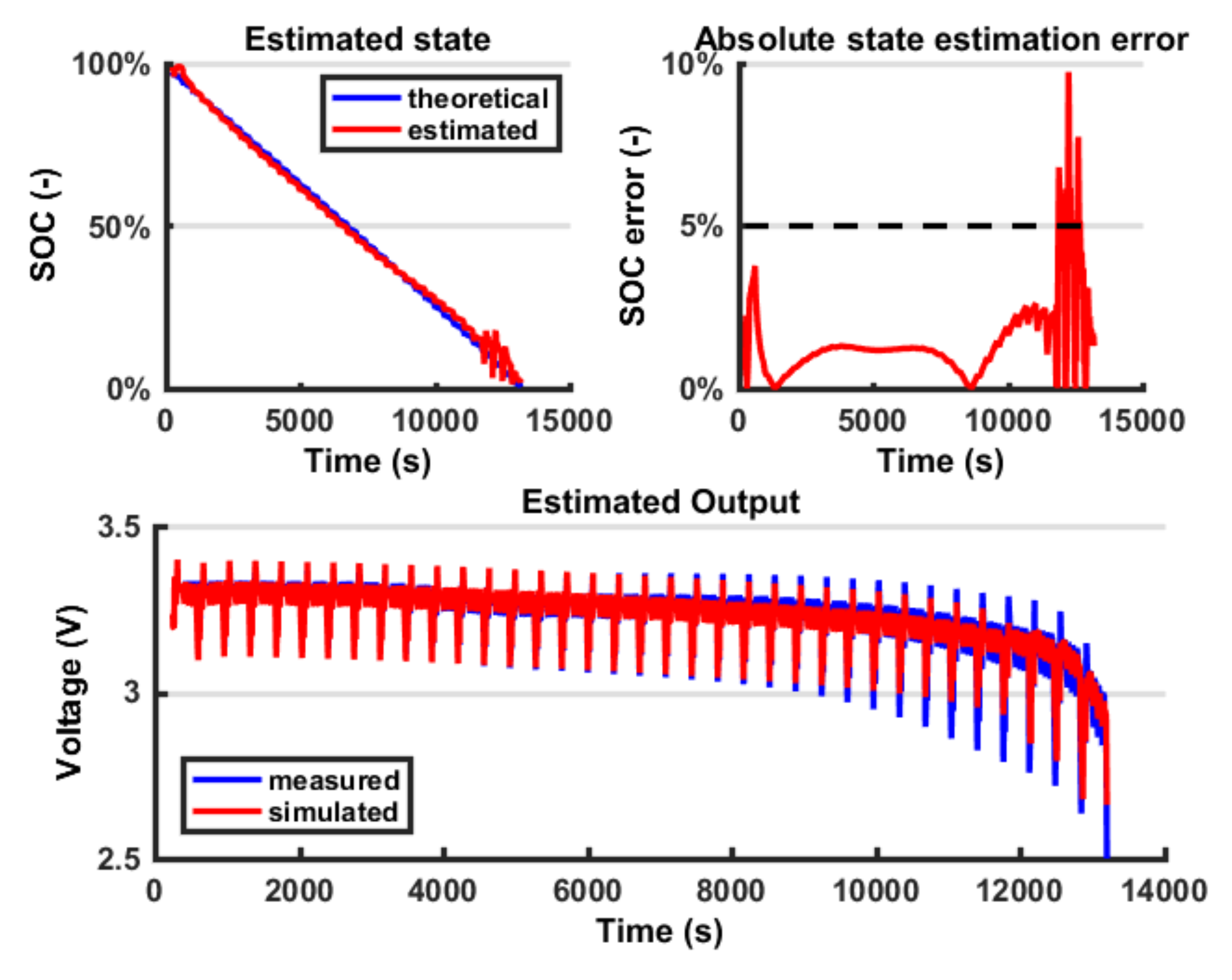
Figure 14.
DST output voltage comparison. (a) whole test; (b) zoom.
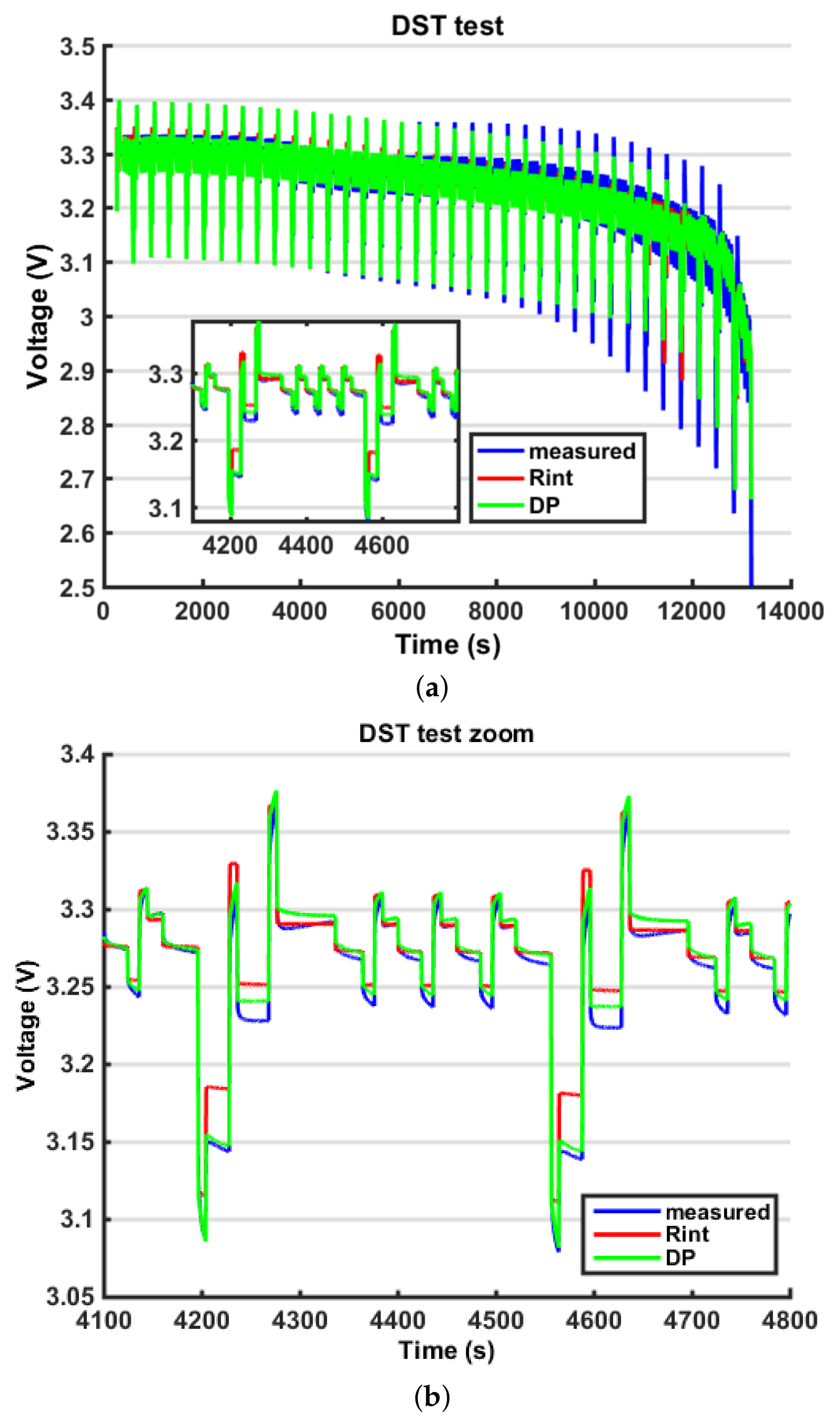
Figure 15.
Modified version of Hybrid Pulse Power Characterization (HPPC) test.
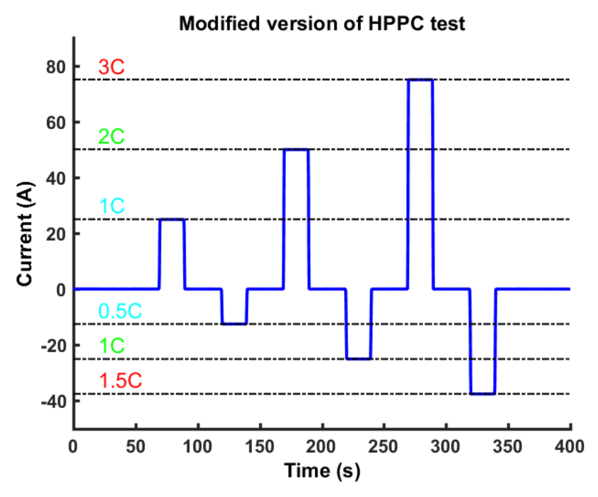
Figure 16.
Combined-Rint model.
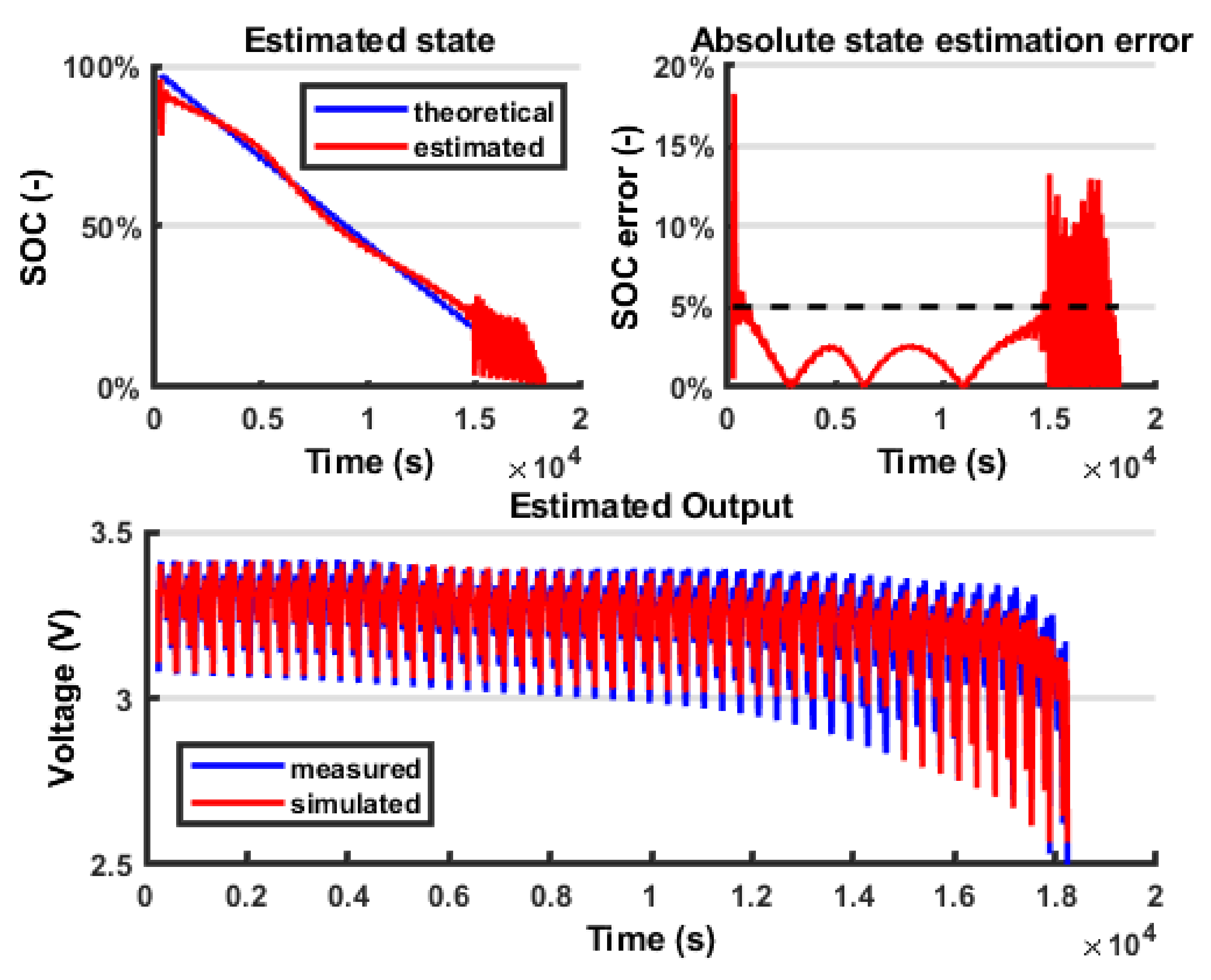
Figure 17.
Combined-DP model.
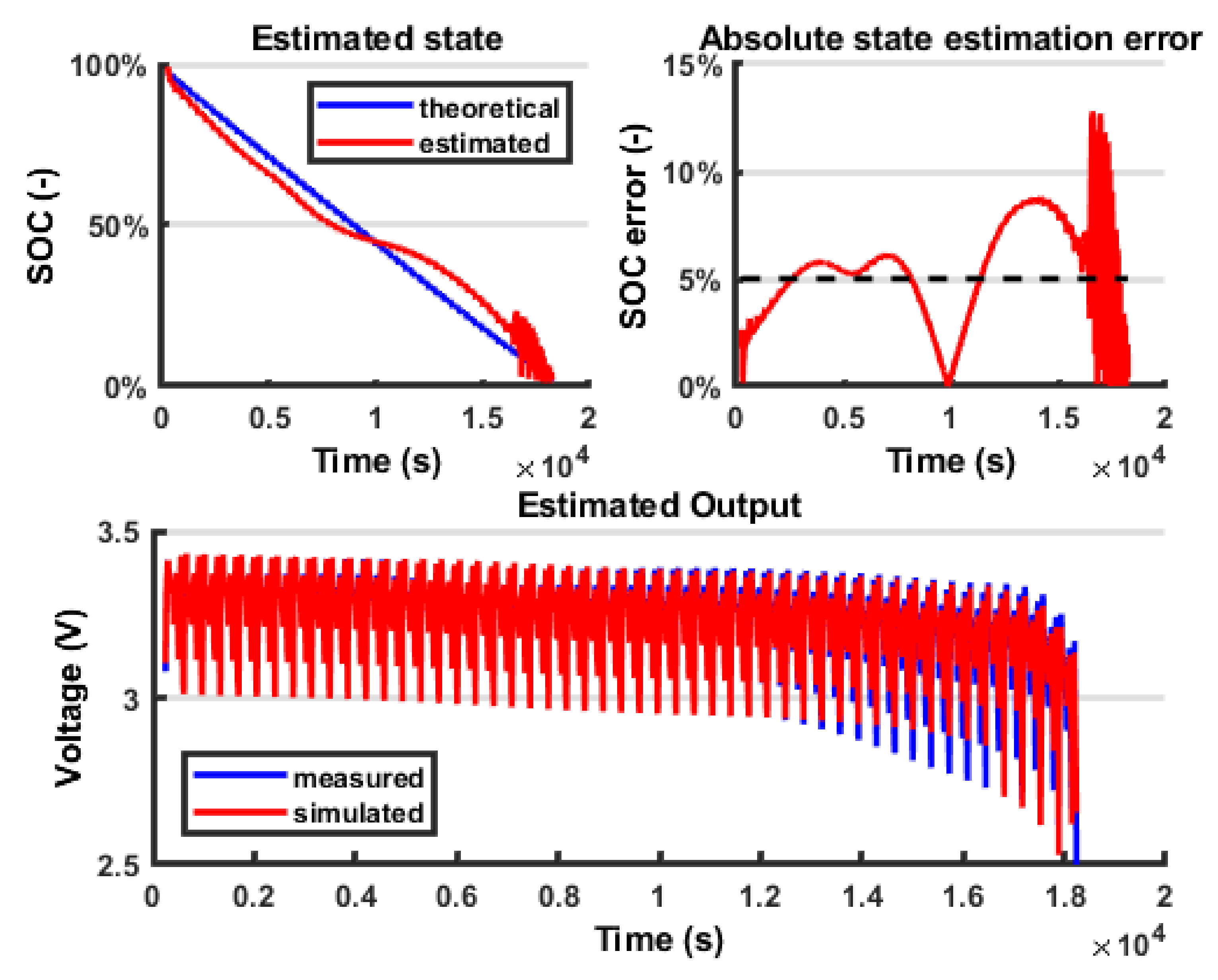
Figure 18.
HPPC output voltage comparison. (a) whole test. (b) zoom.

Table 1.
Cell key manufacturer specifications.
| Specifications | |
|---|---|
| Chemistry | LFP/C |
| Format | Prismatic |
| Dimensions | 70 mm × 180 mm × 27 mm |
| Nominal Capacity | 25 Ah |
| Cut off Voltage | 2.0 V |
| End of Charge Voltage | 3.65 V |
| End of Charge Current | C/20 |
| Max continuous discharging current | 3C |
Table 2.
Model parameters identified by means of the voltage drop method.
| Rs () | Rp1 () | p1 (s) | Rp2 () | p2 (s) |
|---|---|---|---|---|
| 0.0032 | 0.0013 | 13.82 | 0.0015 | 7155 |
Table 3.
Summary of some significant points from the VOC vs. SOC identified relationship.
| SOC (%) | VOC (V) |
|---|---|
| 90 | 3.32 |
| 70 | 3.30 |
| 50 | 3.28 |
| 30 | 3.24 |
| 10 | 3.14 |
Table 4.
Rint-Combined model parameters according to the LSP.
| K0 (V) | K1 (V) | K2 (V) | K3 (V) | K4 (V) | R0 () |
|---|---|---|---|---|---|
| 3.37 | 0.0014 | 0.069 | 0.092 | −0.0087 | 0.0045 |
Table 5.
Open circuit Voltage-Combined model parameters according to the LSP.
| K0 (V) | K1 (V) | K2 (V) | K3 (V) | K4 (V) |
|---|---|---|---|---|
| 3.43 | −0.0019 | 0.155 | 0.097 | −0.025 |
Table 6.
Analysis of the voltage estimation error.
| Model | R2 (−) | MAE (mV) | RMSE (mV) |
|---|---|---|---|
| Rint-Combined | 0.923 | 15.55 | 0.10 |
| DP-Combined | 0.954 | 11.37 | 0.08 |
Table 7.
Analysis of the SOC estimation error.
| Model | R2 (−) | MAE (%) | RMSE (%) |
|---|---|---|---|
| Rint-Combined | 0.939 | 5.694 | 0.028 |
| DP-Combined | 0.995 | 1.475 | 0.008 |
© 2018 by the authors. Licensee MDPI, Basel, Switzerland. This article is an open access article distributed under the terms and conditions of the Creative Commons Attribution (CC BY) license (http://creativecommons.org/licenses/by/4.0/).
Share and Cite
MDPI and ACS Style
Vergori, E.; Mocera, F.; Somà, A. Battery Modelling and Simulation Using a Programmable Testing Equipment. Computers 2018, 7, 20. https://doi.org/10.3390/computers7020020
AMA Style
Vergori E, Mocera F, Somà A. Battery Modelling and Simulation Using a Programmable Testing Equipment. Computers. 2018; 7(2):20. https://doi.org/10.3390/computers7020020
Chicago/Turabian StyleVergori, Elena, Francesco Mocera, and Aurelio Somà. 2018. "Battery Modelling and Simulation Using a Programmable Testing Equipment" Computers 7, no. 2: 20. https://doi.org/10.3390/computers7020020
Note that from the first issue of 2016, this journal uses article numbers instead of page numbers. See further details here.