1. Introduction
Neural networks are ubiquitous as tools for data analysis and processing, finding applications in many research fields and commercial applications including classification problems and image recognition tasks [
1]. The scale of these artificial neural networks has grown substantially in recent years, driven largely by increases in processing power and memory capacity; some of the largest networks now comprise several thousand neurons, with some research using millions of connections. The increase in scale has also enabled more complex and powerful neural networks to be constructed, and there is a continuing drive to produce even larger networks. As a result, the design of efficient and effective hardware implementations is an important research topic [
2]. Furthermore, Moore’s Law and the fast approaching physical transistor scaling limits mean that new technologies and design paradigms must be developed to allow the continued improvement of processor technologies. To date, this rapid advancement in processor speed and scale, which has previously driven significant progress in neural networks, has been mainly achieved through the continued scaling of transistors. As this trajectory reaches its long predicted end, designers and engineers must look to other sources of inspiration, such as that of the human brain, to provide future improvements in computing power [
3].
The apparent efficiency and efficacy of biological neural networks is an attractive trait, and the modelling of such networks must play a key role in the development of improved artificial neural networks. Biological experimentation often involves costly medical procedures. Modelling of biological networks can complement the existing biological experiments or ‘wet work’, saving both time and money when testing new hypotheses. There are many hardware architectures that have been developed for neural simulation. Importantly however, most of these systems assume full global connectivity between neurons. As a result, they frequently use packet-switched networks and time-division multiplexing to connect neurons together. This differs significantly from the structures seen within nature, which typically present localised processing and communications with a smaller number of long global connections. The
Caenorhabditis elegans (
C. elegans) demonstrates this locality, with very few globally connected neurons [
4]. Considering larger animals, such as rodents and small birds, it is observed that this natural dividing of nervous systems into smaller sub-systems is continued. Thus, it is possible to emulate parts such as a bat’s auditory system without needing to simulate or even understand the animal’s entire nervous system [
5].
This paper presents two reconfigurable architectures that are designed with differing levels of communication locality in a manner that is technology independent and inherent to each architecture. Such abstraction is designed to enable the rapid implementation of different neural networks using the two architectures. A demonstration and validation of both architectures is presented using a full model of the C. elegans locomotive system. The first architecture in this paper is a hybrid-local architecture, meaning that it uses connection locality to complement the global connection infrastructure. This architecture uses a more traditional globally connected bus infrastructure, adding locally connected synapses to reduce the bus utilisation. The second architecture is fully local and supports local connectivity throughout its fundamental structure, allowing only a small number of global connections.
Section 2 presents an overview of the research field and highlights existing systems and publications.
Section 3 introduces the two architectures, highlighting their differences and relative merits.
Section 4 introduces the methodology used to validate the two architectures, introducing both a 2D and 3D
C. elegans physical model that allows for direct visualization of movement as a result of neuron simulations. The results of these tests are presented in
Section 5, before a comparison of the scalability of both architectures is considered in
Section 6. A speed improvement of up to 17.5× for a 50 segment
C. elegans locomotive model is shown when implemented on a fully local system. Finally, a discussion considering the impact and relevance of network locality is provided in
Section 7, with the conclusions highlighted in
Section 8.
The critical contributions of this work are the introduction of two novel architectures, supporting hybrid-local and fully-local connection infrastructures; the discovery that locally connected architectures can realise signifiant speed and scalability improvements over their hybrid-local and global counterparts; a demonstration that Convolutional Neural Networks, which appear to contain a high degree of locality within their connectivity, map poorly to locally connected architectures; and the identification of differences in artificial and biological system dimensionality, revealing that both the connection infrastructure and underlying technologies require careful consideration when using biology as inspiration for new systems.
2. Background
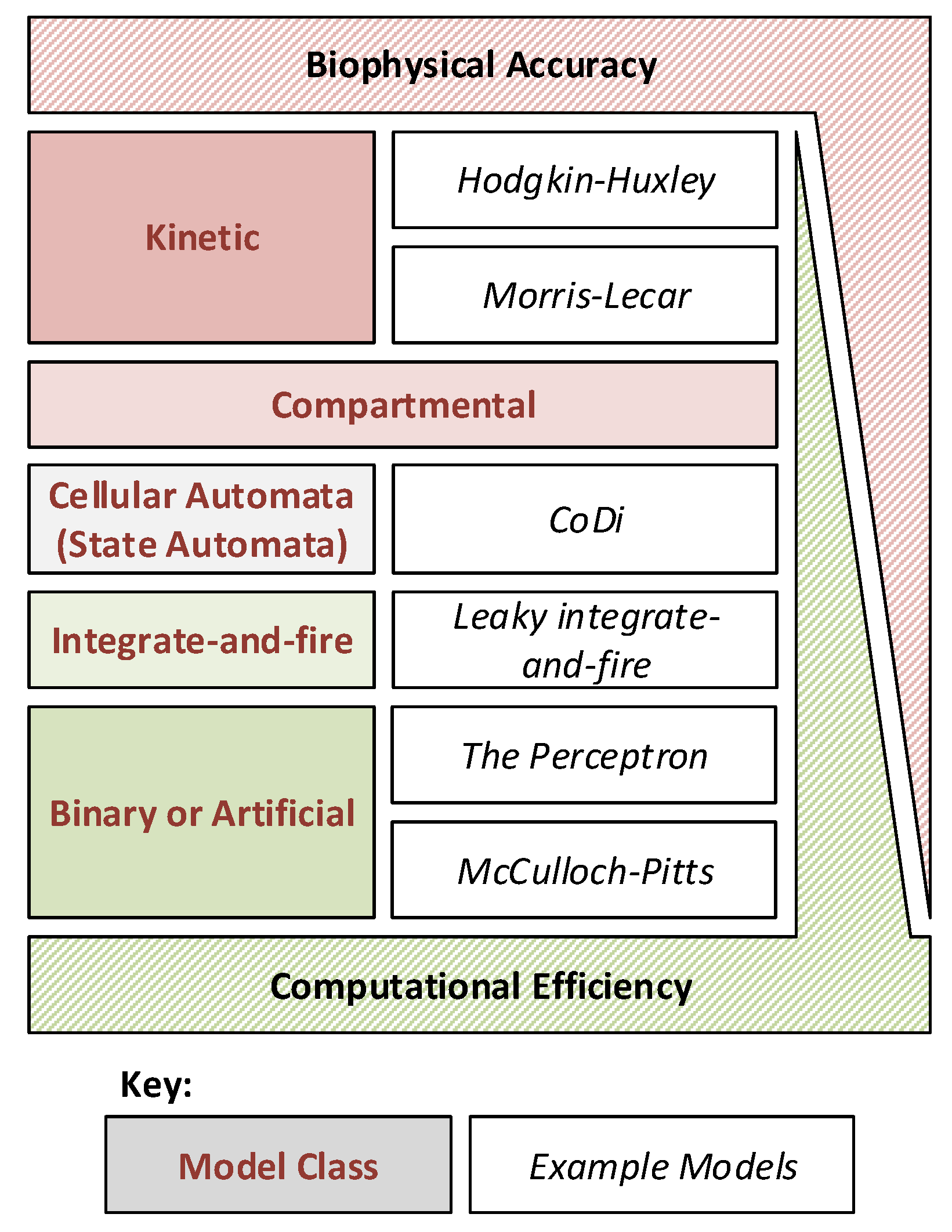
There are many models available for both biophysical and computational neural network emulation. These models must perform a trade-off between biophysical accuracy and computational efficiency, as shown in
Figure 1, and selection of a suitable model is often dependent on the end application and research purpose. Biophysically accurate models (such as Kinetic models like the famous Hodgkin–Huxley model) are often required when investigating the function of single neurons, or small neural networks. At the other extreme, computationally efficient but somewhat approximative models (such as binary or integrate and fire models) have provided significant advancement in large-scale neural network performance due to their simplicity.
Despite the variation from one neuron model to another, the communication infrastructure used to link them together into large neural networks is often more consistent in design. Global connectivity (that is the ability to connect any neuron to any other neuron) provides the greatest flexibility for reconfigurable architectures, and therefore is often assumed as a requirement in the design of neuromorphic architectures.
2.1. Hardware Neural Network Systems
Packet-switched networks are the most common communication method used to pass signals from one neuron to another, with each packet typically containing the firing neurons identity and time of excitation. One such packet-switched network system is SpiNNaker [
6]. Structured as a Globally Asynchronous Locally Synchronous (GALS) system, it is constructed from custom designed Integrated Circuits (ICs) that contain 18 ARM968 processors surrounded by a light-weight packet-switched asynchronous communications infrastructure. These custom ICs are connected together in a 3D torus structure in an effort to reduce the maximal distance between any two points. Custom ICs have long development cycles of approximately 6 to 12 months and high costs in the range of £500,000 per prototype run; long-term manufacturing is far more economic but rarely applicable to research systems. Another constraining factor of this design is the communications channel, with implementations of highly active large-scale networks requiring significant bandwidth. This bandwidth requirement creates a choke point in the system, slowing the speed at which simulations can be performed. In the worst case, this can also lead to dropped packets within the communications infrastructure, meaning that signals and data can be lost during simulation.
To avoid the issue of communications bottlenecks, unique connections in an all-to-all configuration can also be used. Such systems typically make use of cross-bar arrays and memristor structures to provide reconfigurable hardware interconnects in a small silicon package [
7,
8]. These systems yield the fastest neuron to neuron throughput; however, they scale at a rate of
making them unsuitable for large-scale networks of several thousand neurons. They will also contain significant redundant connectivity for any given application as many of the connections will go unused in a typical neural network.
Some hybrid systems, such as TrueNorth [
9], offer a mix of local and global connection infrastructure in attempts to reduce the unused connection count while limiting the long-distance communications bottleneck. These systems still provide global connectivity; however, they use the local connection infrastructure to complement the global communications infrastructure and avoid its over-utilisation. TrueNorth, another GALS system, also uses time-division multiplexing to allow a single computational unit to calculate the outputs of 256 logical neurons. These neuron outputs are then connected locally through a 64k synaptic crossbar array. The interchip connections are handled by a packet-switched network providing the full global connectivity.
2.2. Biological Inspiration
Despite the wide use of global connectivity in neuromorphic systems, biological neural networks are not globally connected; instead, they have properties similar to that of organised circuits [
10]. Designing a system with similar locality constraints may make it possible to produce a resource efficient hardware system that is still capable of fully representing networks and functions seen in nature. Such work stands to benefit both biophysically accurate experiments and computationally efficient systems by reducing the resource requirements; however, these benefits are more significant in large-to-massive scale artificial networks where small improvements to the underlying architectures can have compound effects on the systems as a whole. Using connection constraints can reduce the risk of communications bottlenecks while supporting system scalability; however, the level of connectivity support required must first be investigated for such systems to be effective. The two reconfigurable neural architectures described in
Section 3 use computationally efficient neural models and were designed with two different levels of connectivity to support the comparison of hybrid-local and fully-local network performance.
3. Proposed Architectures
As a form of rapid prototyping, the architectures described in this paper were implemented on a Field Programmable Gate Array (FPGA); an FPGA is a reconfigurable hardware IC that uses lookup tables and connection logic to allow engineers to define and implement custom hardware systems rapidly without the high cost typically associated with custom IC design. These devices use Hardware Description Languages (HDL) such as VHDL or SystemVerilog to define the desired arrangement of gates and registers and a synthesis tool then computes a mapping to allow the defined system to be implemented on the FPGA. This is distinctly different from running software on a processor as the HDL is used to connect physical hardware together to form a circuit rather than generate a set of processor instructions.
3.1. Architecture A—The Column Architecture
The first architecture, termed the column architecture, is based on work by Bailey [
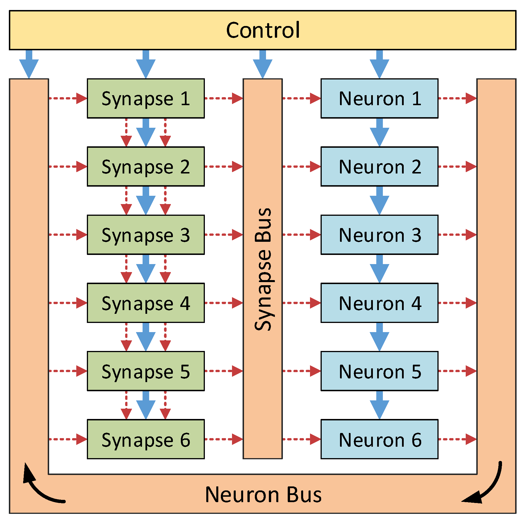
11] and makes use of hybrid-locality to reduce the communications bottlenecks. This column architecture is a reconfigurable neural hardware system capable of real-time simulation of neural networks. Designed using custom VHDL building blocks, the system may be programmed to simulate a desired network using a set of configuration words. In order to reduce the connectivity requirements, the neurons and synapses were developed as separate blocks and conceptually arranged into two columns, as shown in
Figure 2. This allowed a novel local connection infrastructure to be used within the synapses, reducing the global bus communication requirements.
The neuron blocks were designed to operate in two modes, as either a base neuron or a pattern generator. In the base neuron mode, the neuron takes input from the synapses, passes it through a threshold block and triggers a burst generator if the threshold is exceeded. In the pattern generator mode, the input is replaced with an internal oscillator that triggers the the burst generator at user defined intervals.
These two modes may be programmed by the end user using the pre-defined configuration words, shown in
Table 1. As such, this model allows the end user to customise the neurons contained within the network without requiring a detailed understanding of VHDL.
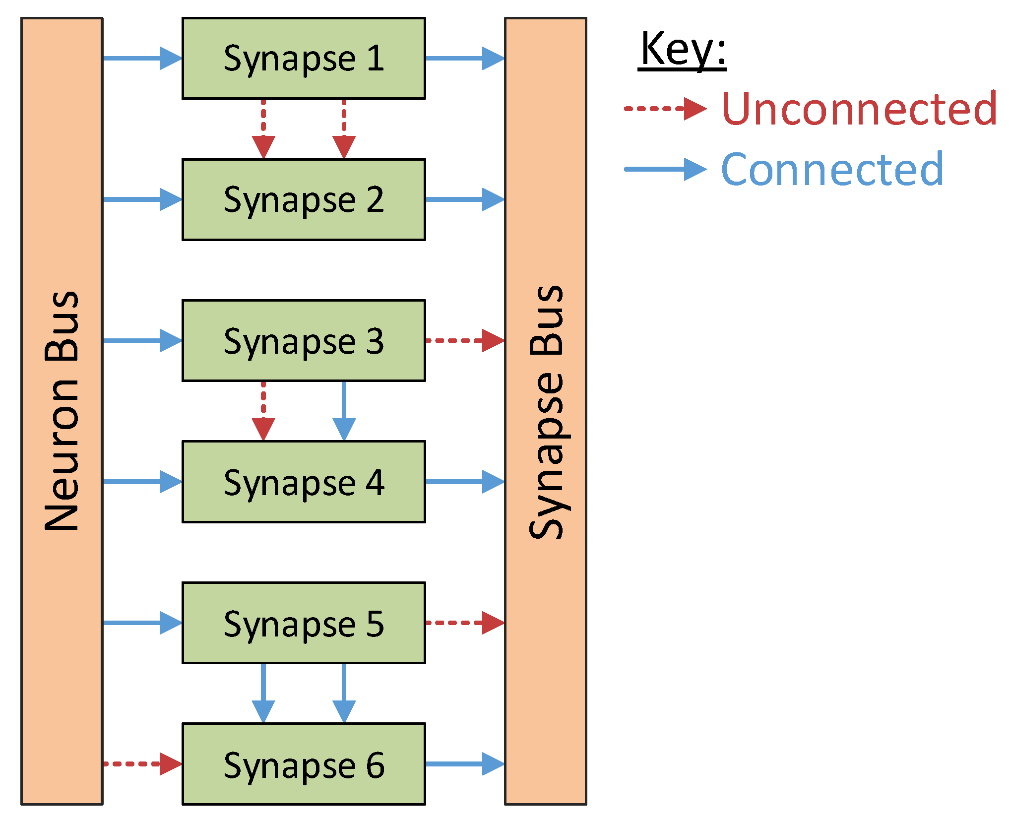
The synapse blocks perform the bulk communications within the system. Designed to support connections to the neighbouring synapses at both the input and output sides of the block, these synapses perform the summing operations for the various neuron stimuli while also providing a way for multiple synapses to be triggered concurrently by the same neuron. These local internal connections within the synapse column reduce the communications between the synapse and neuron columns considerably as each neuron need listen to only one synapse within the system. The various configurations these connections support are shown in
Figure 3. Synapse 1 and synapse 2 are not connected in any way; synapse 3 has its output connected to synapse 4, meaning that synapse 4 will output the sum of the two synapses; and synapse 5 is connected to synapse 6 at both the input and output stage. This last configuration allows a synapse to be activated by a pre-synaptic neuron even while the synapse is already active.
As with the neuron blocks, the synapse blocks are fully configured using the configuration word detailed in
Table 2. This configuration is performed alongside the neuron configuration and once again allows full use of the system without prior knowledge of VHDL.
The neuron and synapse columns are connected together by two buses. These buses are global connections, allowing any neuron to connect to any synapse and vice versa. At any time, only one neuron and one synapse may drive the neuron and synapse buses, respectively; however, many neurons and synapses may listen to these buses at the same time. To ensure that these buses are not multiply driven, a global controller is used that cycles through the address space. The neuron (or synapse) that contains the active output address drives the neuron bus (or synapse bus) for that clock cycle, and any synapses that have the same address in their input address register will listen to the bus for that clock cycle. In this way, the neuron and synapse bus use time-division multiplexing to appear fully transparent to the system, allowing full global connectivity. Since the system must cycle through all neurons in each simulated time step, the maximum system simulation clock frequency,
, is impacted by the number of neurons simulated,
n, and may be found using Equation (
1), where
is the internal system clock frequency:
This clock scaling creates significant problems when simulating large neural networks of several thousand neurons. Since each neuron must drive the bus once per simulated time step, the simulation clock must run much slower to accommodate for the increase in scale. This system is therefore not scalable; however, by ensuring that synapse to synapse connections were performed outside the scope of the wider connection infrastructure, this system achieved measured speed-ups of 20× that of previous models it was compared against [
12].
3.2. Architecture B—The Grid Architecture
A second novel architecture (the gird architecture) was designed as an example fully-local architecture. Using this local connectivity, it yields a system that may be scaled easily in two dimensions without directly impacting the system speed. In this architecture, the neurons and synapses are brought back together into a single block or node. These nodes are arranged in a 2D grid and connect in a North, East, South, West fashion to their direct neighbours using a custom connection infrastructure.
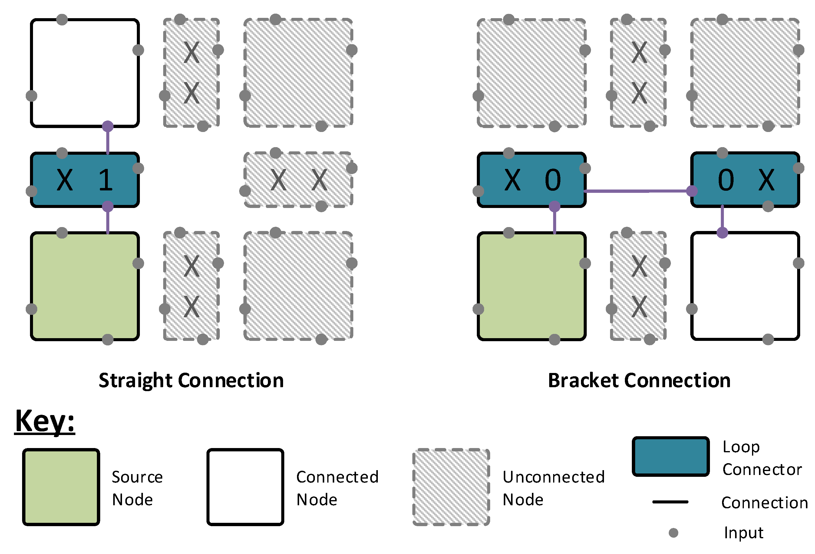
As shown in
Figure 4, this connection infrastructure sits between the nodes and re-directs the incoming signals according to user-defined configuration bits. This allows the nodes to be arranged into loops, with each neuron able to connect to a total of four different loops—one on each face. The loops are latched internally within the nodes, allowing all nodes to drive their loop segment at all times. A global controller cycles through an address space, 0 to
m, where
m is the size in nodes of the largest loop in the network. At address 0, the nodes drive their outputs onto the loop, passing them along to the next node in the chain. For all other addresses, the nodes simply pass the data around the loop, progressing once for each address increment. The nodes then use internal registers to determine when to listen to the loops, allowing any node to receive input from any other node in a shared loop. In this fashion, no node is more than one intermediate node away from any other node in the system. This architecture benefits from requiring a smaller control address space than that of the column architecture, meaning that a network simulation speed is dependent on its largest loop size rather than the network size itself.
In order to interface with external systems and provide some global connections outside of the loop arrangement itself, Input/Output (IO) blocks were added to the grid. These IO blocks sit on the loops, replacing a node. As with the nodes, they are able to drive data into the loop and read data from the loop; however, they also have an external communications point that connects to an external pin on the IC package. These pins may be connected to sensors or actuators, providing IO for the network, or they may be connected to one another, acting as a long range connection that operates outside of the neighbourhood domain.
The nodes themselves can support a broad range of different neuron models (any of those given in
Figure 1). In this work, and for simplicity, a configurable integrate and fire model was used. This model contains internal weights that are applied to the incoming stimulus. The weighted input is added together and passed through a threshold block and, if the threshold is exceeded, the output is set high ready for the next loop cycle. All loop cycles are kept in synchronisation, meaning that smaller loops shut down once finished while waiting for the larger loops to complete their cycles.
This grid architecture is configured, as before, using configuration commands. These are sent along a serial control bus that connects to a computer to allow the configuration and monitoring of the system during use. These configuration commands set the connection infrastructure arrangement, the node weights, IO direction and the controllers’ address space range. In a technique similar to that of FPGA synthesis engines, it is up to the network synthesis tool to arrange the network and fit the neurons into neighbouring node loops, with an aim to minimise the maximum loop size.
Both of these architectures require an internal clock and controller that propagates fully through an address space once for each simulated time-step. While the column architecture requires each neuron to have a unique address, the grid architecture requires neurons to only have unique addresses within any given loop. As such, many neurons may drive independent loops at the same time, reducing the total cycle count required per simulated time-step. This grid architecture is described in further detail by Graham-Harper-Cater et al. [
13].
4. Validation Methodology
The two architectures’ representation abilities were first validated using a model of the full locomotive system of the
C. elegans. The resulting neural networks were used to drive a 2D and 3D model to provide a visual representation of the resulting rectilinear locomotion. The
C. elegans was selected for this process as it is the only living organism to have had its connectome (the neuronal ’wiring diagram’) fully mapped [
4]. Existing models of the locomotion system were available for verification of the results [
14,
15,
16,
17]. There are also many video recordings of the animals’ locomotion readily available online.
4.1. The C. elegans Locomotive Model
The
Caenorhabditis elegans (
C. elegans) is a transparent free-living nematode that is approximately 1.3 mm long, takes 3.5 days to maturate and has a total of 302 neurons [
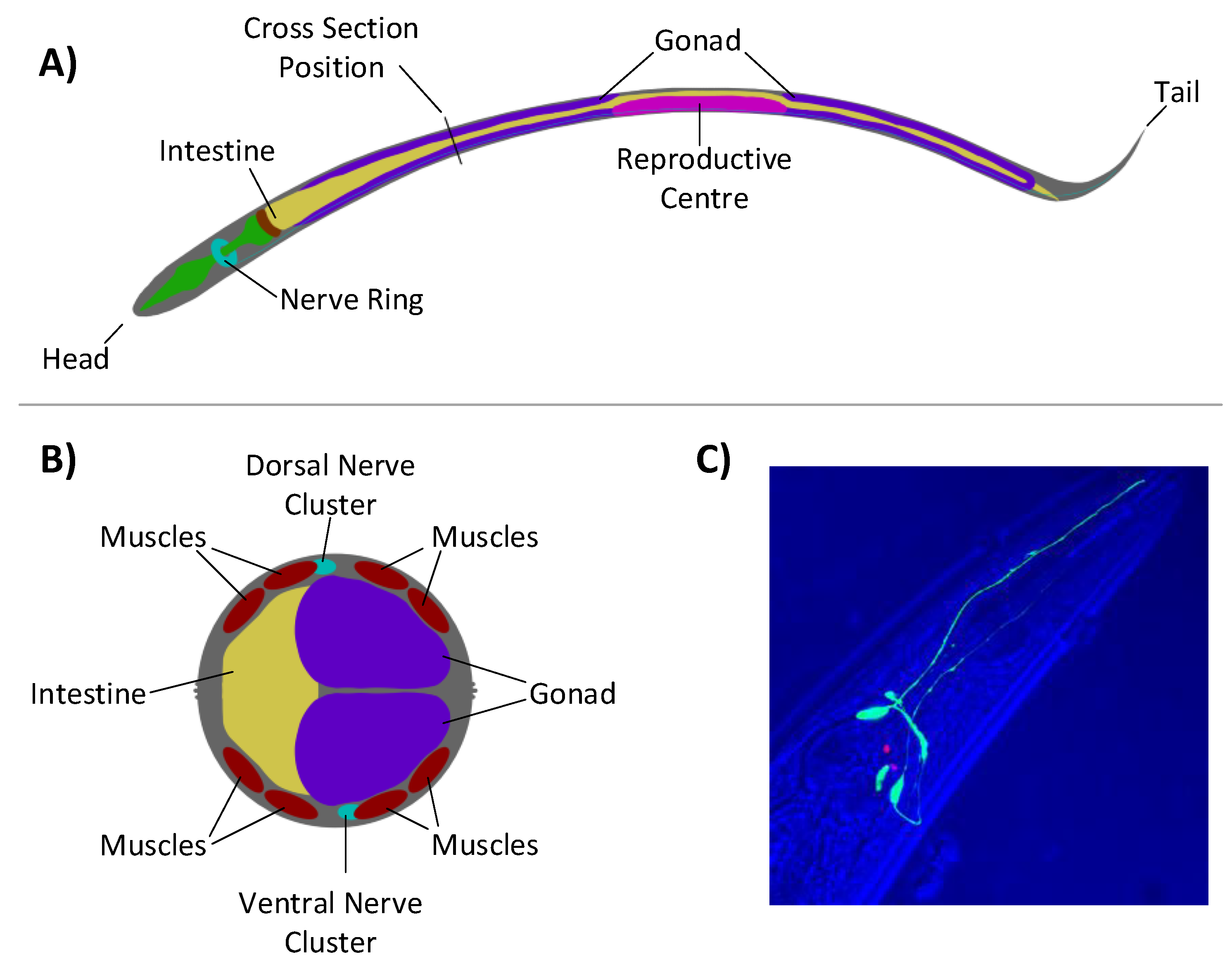
4]. The animal moves forwards and backwards in a serpentine fashion using rectilinear locomotion to locate food and escape predators. It may also exhibit coiling behaviour in the event of a sudden stimulus to the animals’ side. It has a muscular structure built up of eight distinct regions that run down both sides of its body as shown in
Figure 5. These muscles are used to produce locomotion through sinusoidal activation which propagates down the animal in a synchronised fashion.
First introduced by Claverol [
14], the
C. elegans event-based locomotive model simulates a small part of this animals connectome, containing only 86 neurons and 180 synapses. This neural circuit is responsible for the forward and backwards locomotion as well as coiling behaviour.
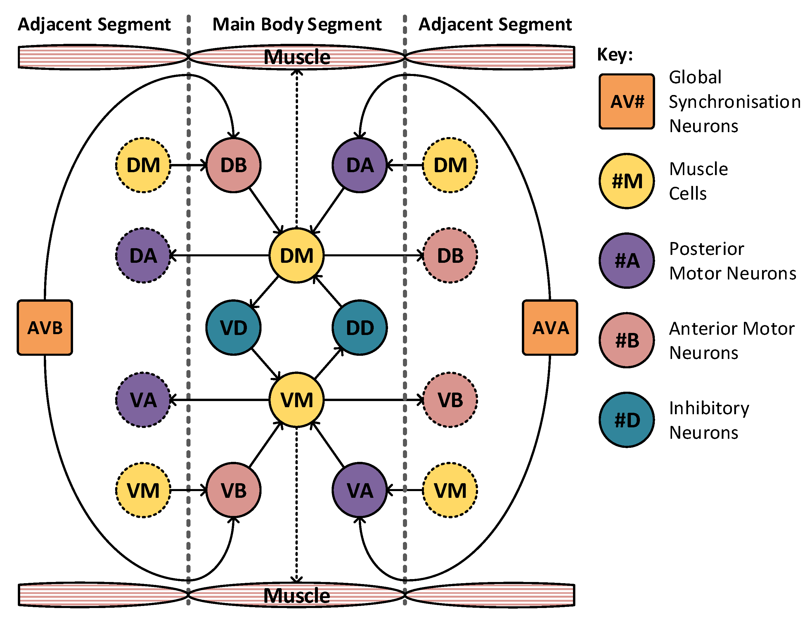
The model may be divided into 10 segments to match the animals nervous system itself. The majority of these segments take the form shown in
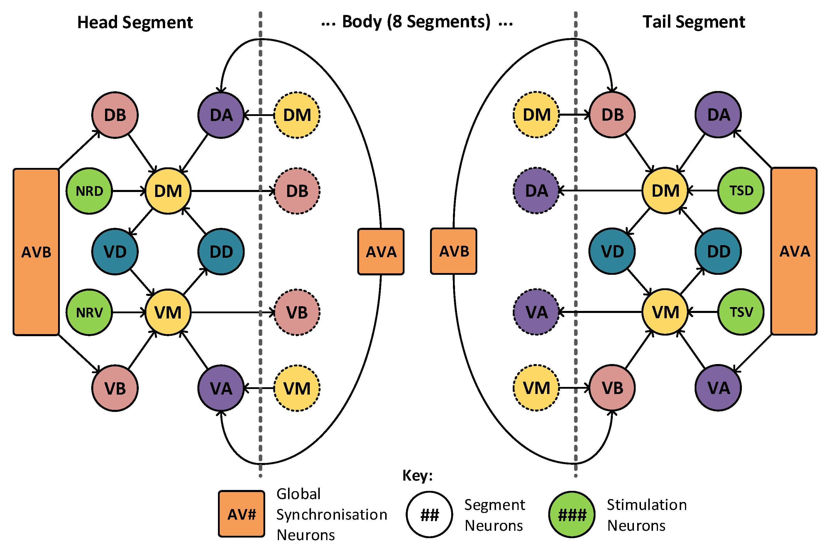
Figure 6, where there is a high level of locality within the model. The muscle cells, denoted DM and VM, drive muscle activation within their respective segments. These are triggered by the motor neurons in adjacent segments, labelled VA, VB, DA and DB. These motor neurons require concurrent activation from both the muscle cells and the synchronization cells, marked AVA and AVB. The two remaining neurons, VD and DD, operate as inhibitory neurons and are responsible for the contralateral inhibition of the muscle on the opposite side of the animal. In this arrangement only, a limited number of connections join to adjacent sections and a total of two neurons (AVA and AVB) are connected globally, joining to all segments. The head and tail segments have two additional neurons each (marked NRD, NRV in the head and TSD, TSV in the tail), to act as stimulation points for the rest of the locomotive system. These extra neurons may be seen highlighted in green in
Figure 7, which shows the construction of the head and tail sections of the locomotive model. Each of these stimulation neurons represent separate neural systems, which, combined, guide the animals locomotion. In this model, these neural systems are replaced with a set of frequency controlled oscillators that generate the desired stimulus input frequencies. The eight distinct regions of muscle shown in
Figure 5 are grouped into two sets: the dorsal set and the ventral set. These are then treated as a singular muscle with just one dorsal and ventral motor neuron driving each set per segment, as shown in
Figure 6.
This event-driven model has been utilised in numerous different implementations for neural hardware [
14,
15,
16,
17]. These models provide resultant behaviours that new systems may be compared against to ensure functional equivalence and make the locomotive model a practical test for new reconfigurable architectures, providing a simple yet functionally verifiable network inspired by nature.
4.2. Architecture Representation Validation
The C. elegans locomotive model was implemented on an FPGA, independently using both the column and grid architecture. This provided a direct validation and verification mechanism. With the reconfigurable architectures built, configuration files were generated to describe the locomotive model on each architecture. While such configuration files would nominally be generated by a synthesis engine, the ones used in this test were defined by hand. This was done to ensure that the architectures themselves were tested fairly without external influence from any synthesis algorithms or hidden layout decision processes. Synthesis and system fitting are two concepts well established within FPGA and Custom IC development and therefore are of limited interest when verifying the architectures fundamental ability to represent a problem or task.
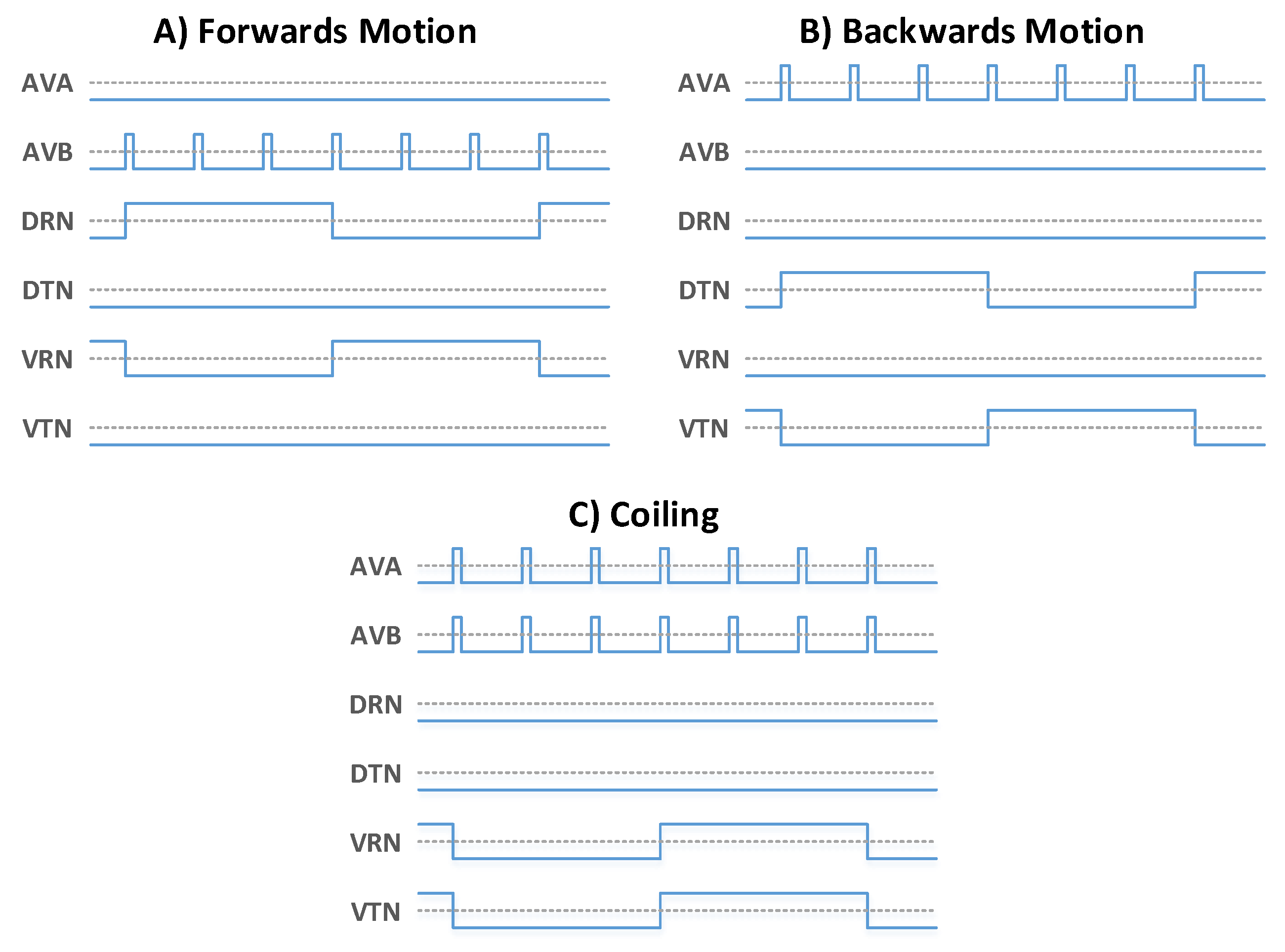
HDL test bench files were developed and run in Modelsim to apply these configuration files and then simulate the stimuli as seen in the animal. The test bench was designed to wrap around the architecture-under-test, connecting to the IO blocks and the control/programming interfaces. This allowed the architecture to be reconfigured on command, providing monitoring for the output signals and direct control over the input stimuli. The stimuli for forwards, backwards and coiling behaviour are shown in
Figure 8. Each locomotive behaviour is selected by generating the associated oscillation signals at the AVA, AVB, DRN, DTN, VRN and VTN neurons as shown. The test bench was configured with custom control signals to easily select and generate the desired stimuli on command. These input stimuli each yield a predictable motor response, and therefore the test bench was setup to record all motor neuron outputs for verification. These recorded motor neuron signals were then written to file to support further investigation and validation.
The test benches were configured to test for forwards, backwards and coiling behaviour as seen in a healthy animal. Since the system is easily configurable, gene knockout tests may also be performed. The UNC25 gene knockout mutation causes the Dorsal and Ventral motor neurons to latch into a constant firing mode when activated. This causes the animal to seize up, resulting in a slight shrinking behaviour. This UNC25 knockout mutation is also implemented and tested on both systems, demonstrating a practical application of reconfigurable hardware systems in neurological research.
4.3. 2D Mechanical Model
In order to further validate the architectures, a new 2D mechanical model of the
C. elegans was developed. Since the
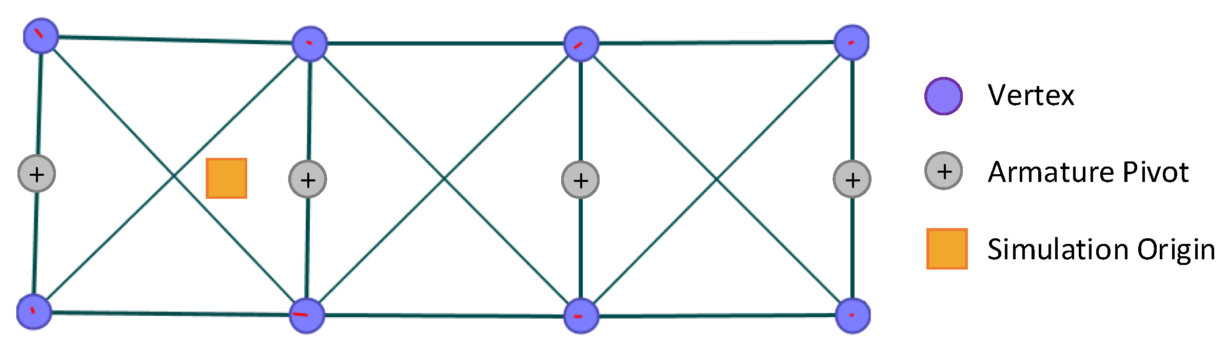
C. elegans is a soft-bodied creature, this mechanical model must act to maintain the animal’s structure while also applying deformation in the event of muscle activation; this model was built using principles from force-directed graphs. As shown in
Figure 9, vertices were placed at equal distances along the length of the
C. elegans, conceptually representing the ends of the muscles. Edges were drawn between neighbouring vertices along the length of the animal, representing the muscles responsible for locomotion. Finally, cross-bars and vertical struts were added to ensure that the simulated mass maintained its structure when force was applied by the muscles.
Each of the edges are treated as linear springs with non-zero resting length,
. Connected vertices are therefore attracted to one another using Hooke’s law as shown in Equation (
2), where
is the force applied to a vertex that is connected to another vertex by an edge of length
l with a spring constant
. The unit vector
points towards the second vertex in the calculation:
While all edges operate as spring attractors, they may be conceptually separated into two categories. The first class are those that operate as muscles and sit alongside the animals; the second are those that act as structural supports for the model. These structural edges maintain a fixed resting length throughout the entire simulation. The muscle edges, however, are modified by muscle contraction, with activation causing the resting length (
) of the edge to shorten and relaxation causing the length to restore to its default value. This length modification is not instantaneous, using a simple feedback loop to control the length change at any simulation time step. This helps ensure that the motion is fluid and also more accurately represents the way muscles contract in biological systems. This feedback loop is shown in Equation (
3), where
represents the muscles activation and is 0 when activated or 1 when relaxed,
is the relaxed resting length of the muscle,
is the current length of the muscle,
is the next muscle length, and
is the muscle constant used to scale the muscles response to stimulus:
The vertices of the model are repelled from one another to ensure that the model doesn’t collapse during muscle contraction. This force is calculated using an inverse square law to ensure that its effect is minimal for all but very close vertices. In this simulation, a form of Coulomb’s law was used to provide this vertex repulsion, as shown below in Equation (
4), where
is a constant,
and
are virtual charges to control a vertex’s influence on the model,
d is the distance between the two vertices in question and
is a vector which points towards the other vertex in the vertex pair under consideration:
The law of conservation of momentum may then be applied to calculate the acceleration caused by the superposition of these forces as shown in Equations (
5) and (
6). In these equations, the vectors are given a mass,
m; the total spring force,
and the total vertex repulsion force,
are calculated; and the velocity
v is used with a drag constant
:
This acceleration value may then be used to calculate the new velocity of the vertex at each time step, ensuring that the system finds equilibrium at rest.
This mechanical model was designed to read the raw ventral and dorsal muscle activation signals produced by hardware architectures on the Modelsim test benches. These activations were stored by the test bench as time-synchronised boolean values representing motor neuron activations. These motor neuron signals were linked to the associated muscle length using Equation (
3). Once the simulated motion was generated, the angles made between segments is then calculated and saved to support the 3D model actuation.
4.4. 3D Model
A new 3D model was built to allow direct visualisation and comparison of the animal’s movement. This simulation makes validation of the neural model easier as it provides a visual representation of the results that may be compared against the biological counterpart. This model was built using a 3D modelling and animation package (Blender was used for this work, available at:
http://www.blender.org) and rigged with a simple linear armature. Each bone in the armature represents a segment along the animal’s length. The segment angles generated using the 2D physics model were then imported and applied to the armature, allowing the resultant motion to be simulated and rendered in 3D.
5. Validation Results
As described in
Section 4, both reconfigurable architectures were verified using the
C. elegans locomotive model. First, a stimulus was applied that, in nature, is observed to cause forwards and backwards motion. Then, the coiling and UNC25 knockout behaviours were also tested. The response of the two architectures to this stimulus was recorded and used in a 2D and 3D model to produce a simulation of the locomotive behaviour. This section presents the results from these tests, comparing these results with previous studies and the biological animal where relevant.
5.1. Forwards/Backwards Motion
Each of the architectures was configured with a simulated
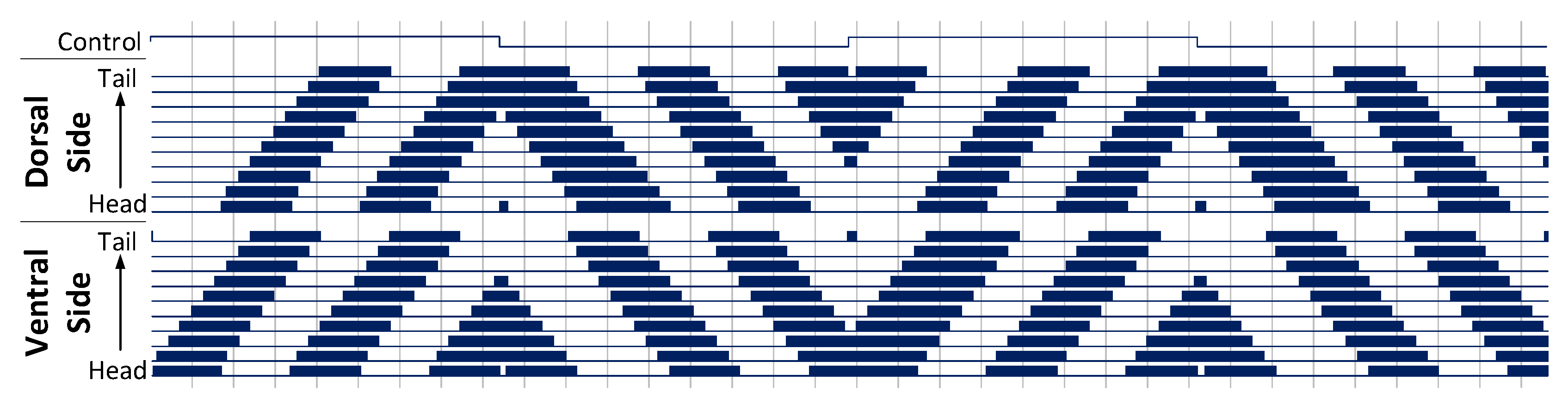
C. elegans with 10 segments. Forwards and backwards locomotion was observed on both architectures using a bi-phasic control signal to produce the appropriate head and tail stimulation. The resulting motor neuron signals generated by the grid architecture are shown in
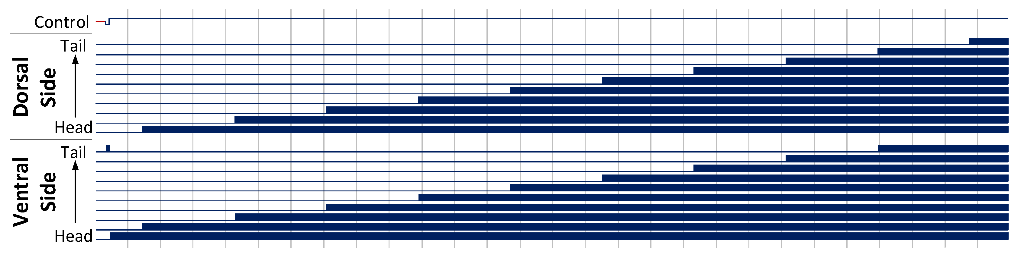
Figure 10. The column architecture results match those of the grid architecture presented here. The top-most trace in this figure is the control signal used to drive the forwards and backwards stimulus. This control signal is set up to oscillate at a low frequency, resulting in an alternating forwards and backwards locomotion.
The top bundle of signals in
Figure 10 form the dorsal muscle cells, while the bottom bundle represent the ventral muscle cells. Activation of these neurons is shown as blocks of colour due to the high frequency oscillations produced by the muscle cells. These neurons are numbered from head to tail starting at 0, such that movement propagating head to tail will move from the bottom to the top of each bundle. Vertical lines are drawn every 500 ms on the
x-axis.
Activity begins on the Ventral side of the head and propagates down to the Dorsal side of the tail, taking approximately 2900 ms to complete one full cycle. These signals produce a sinusoidal motion in the animal, yielding a forwards locomotion.
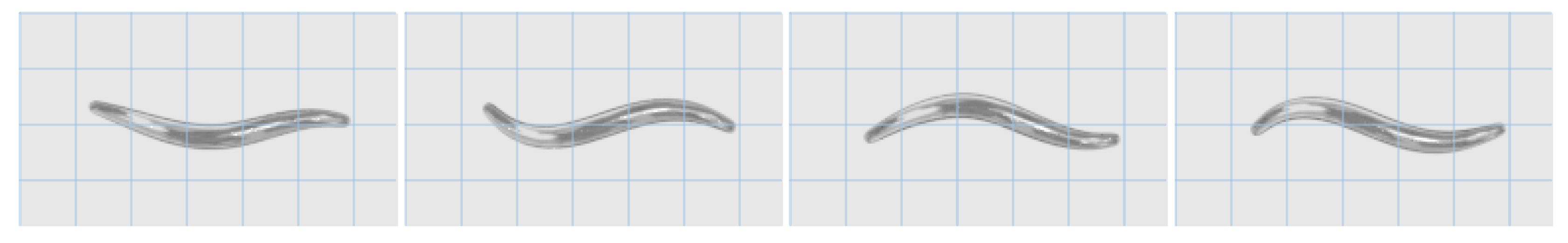
Figure 11 shows frames from the animated 3D model, where this propagating sinusoidal motion is clearly shown.
These results were consistent in both reconfigurable architectures and yields the same propagating waves as seen in previous works and observed in nature. The muscles were observed to oscillate at a frequency of 0.57 Hz which matches the findings of Karbowski et al. [
18]. The propagating muscle signals were found to match those of Claverol et al. [
14] in both shape and structure. The exact timing in the signals varies from model to model, largely due to differences in the timing of stimulation pulses. The works of Mailler et al. [
19], Niebur et al. [
20] and Bailey et al. [
15,
16] all agree on the underlying nature of propagating muscle signals and the resulting serpentine motion. These properties may be seen in both the muscle activation signals moving down the length of the animal and in the 3D model itself. Boyle et al. additionally provide stills from simulations of their model [
21]. These stills were compared against the 3D animation and were found to have the same core locomotive properties. With these comparisons, we are confident that the model is functioning as expected, producing the intended motion.
The locomotive model was mapped onto the grid architecture with a maximum loop size of 10. This means that only nine sub-steps were required to pass all neurons’ outputs to their neighbours within the system and preform a single simulation step. In contrast, the column architecture required all 86 neurons to drive the buses once each for a simulation step meaning that 86 sub-steps were required. This reduction in sub-steps enabled the grid architecture to outperform both the column architecture and previous implementations by a simulation speed increase of
[
13] and allows new segments to be added to the locomotive model without any reduction in performance.
5.2. Coiling Behaviour
Coiling behaviour has also been demonstrated in previous implementations of the
C. elegans locomotive model.
Figure 12 shows the Dorsal and Ventral muscle cells response to a stimulus applied to both the head and tail simultaneously. In this situation, activation begins at both the head and tail of the animal and then propagates to the centre. This muscle activation leads the animal to coil towards the stimulus, which, in this case, was applied to the Ventral side of the animal. The results for this test are consistent between both architectures and produce the expected behaviour. The 3D model was again generated, showing that the signals do indeed lead to coiling behaviour towards the stimulus, as observed in nature. Frames from this simulation may be seen in
Figure 13.
5.3. UNC25 Knockout
Simulations allow researchers to perform rapid experimentation on gene knockout mutations and neuron suppression. The UNC25 gene knockout mutation causes the Dorsal and Ventral motor neuron response to change under stimulus. In this mode, the muscle cells enter a state of constant firing, resulting in a full muscular seizure along the animals length. Applying the standard forward motion stimulus to the head of a
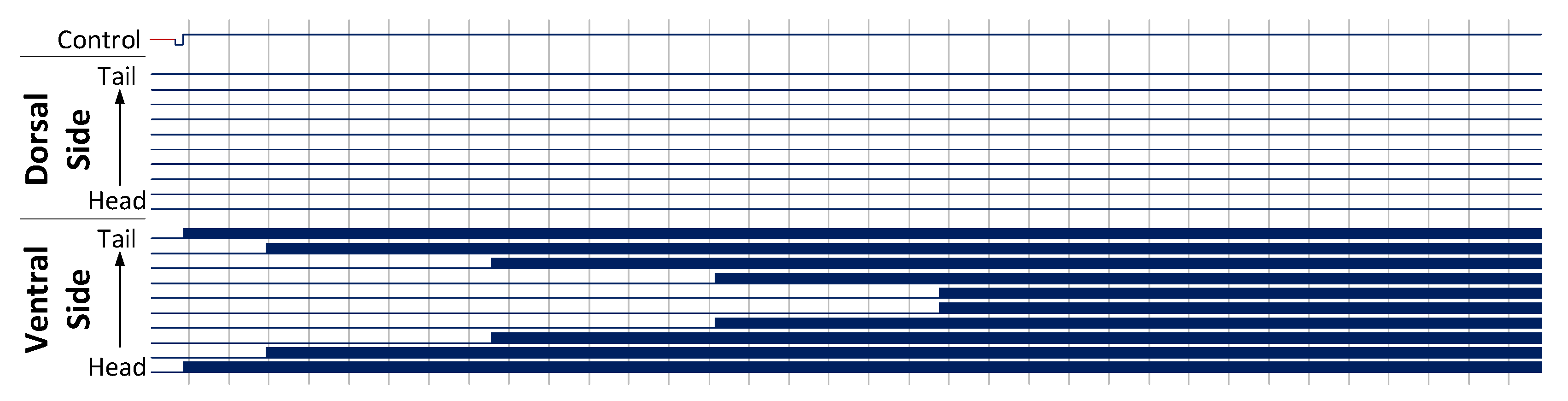
C. elegans with this gene mutation leads to a propagating seizure starting at the head.
Figure 14 shows the motor neuron response to such stimulus. As expected, the mutation results in seizures in the model on both architectures, propagating from head to tail as the locomotive behaviour communicates down the animal’s length.
5.4. Summary
Both the column and grid architecture have been shown to fully emulate the C. elegans locomotive model with no failure or shortcoming in their network representation. The timing and structure of muscle activation waveforms were checked against previous works and found to be in accordance with those results. The 3D model behaviours were also reviewed visually and found to be consistent with observed behaviours seen in nature. Forwards, backwards and coiling behaviour were all demonstrated and the system was shown to be suitable for testing gene knockout behaviour with accurate and biologically correct results.
6. Architecture Comparison
The C. elegans model has been successfully demonstrated on both architectures. An important aspect to consider is the scalability (and its effect on speed) that is possible with each architecture. While the column architecture benefits from supporting a hybrid communications infrastructure, its clock speed is positively correlated to the neuron count. The grid architecture, however, is constrained by the maximum loop size required when fitting the network to the underlying system. Since the 10 segment C. elegans requires 86 neurons and the largest grid loop was 10 neurons, the grid architecture should be faster than the column architecture when implementing the locomotive model.
This performance gain assumes that both systems run with the same internal clock speed. In reality, this is not possible, as different architecture modules will have different clock constraints, as shown in
Table 3. These maximum clock frequencies were generated using the synthesis tools. The grid architecture neurons latch the communications loops, meaning that the communications clock is limited by the neuron clock rate. The column architectures’ neuron clock is also notably slower than the other modules in this table. This difference is due to the way synapses may be chained together within the architecture and represents the absolute worst-case speed, where all synapses are chained together resulting in a large propagation delay. Taking these delays into consideration, the grid architecture was actually only
faster than the column architecture.
The impact of system size on system speed may be calculated by increasing the number of segments used in the
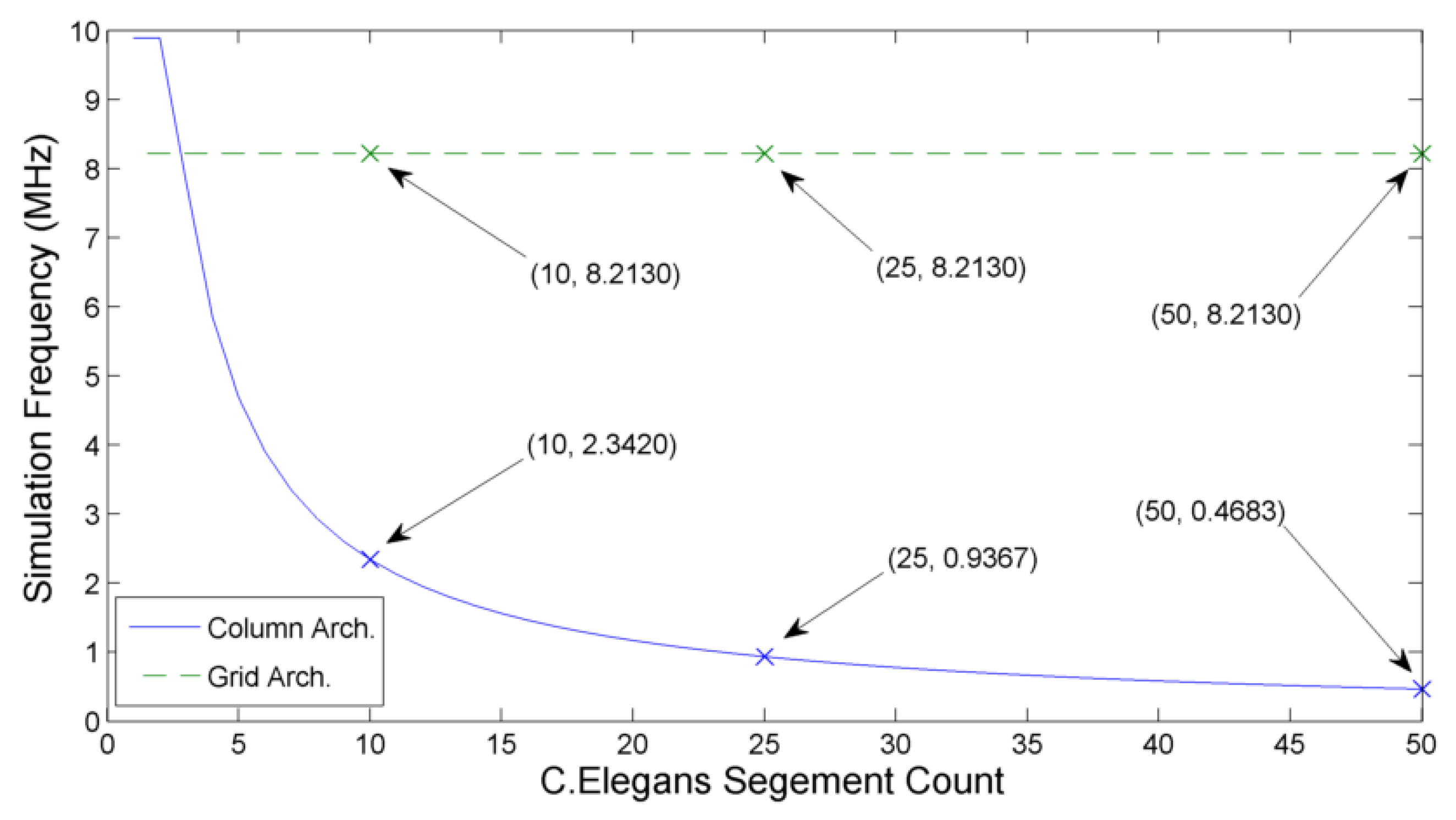
C. elegans model. As shown in
Figure 15, column architecture forms a ‘roof-line’ model, where suitably small networks (such as a 1 segment
C. elegans) are limited by the neuron clock frequency. With the addition of each segment, the total number of neurons simulated is increased by 8. This increase in neuron count causes the simulation frequency to fall away asymptotically towards zero, with the communication frequency now limiting the overall speed.
The grid architecture has a constant simulation frequency as the largest loop size does not increase with the addition of more segments. In
Figure 15, the
gain may be seen in the 10 segment simulation while the estimated
speed improvement occurs when simulating a 25 segment model. Since the hybrid-local column architecture continues asymptomatically, the simulation frequency gain of the grid architecture continues to increase as new segments are added.
This demonstrates how locally constrained architectures can offer significant benefits when simulating systems which also represent a certain degree of locality within their structure. Indeed, a 50 segment C. elegans simulation realises a simulation speed improvement of as much as when implemented on a fully-local architecture.
7. Discussion
The results in
Section 5 show that both a hybrid architecture (such as the column architecture) and a predominantly local architecture (such as the grid architecture) are capable of simulating a naturally occurring network, with a biologically feasible response to gene knockout mutations. Since there are resource benefits to utilising locally connected architectures, it is also of interest to consider how artificial networks map onto such systems.
One of the most popular neural network topologies at present is the Convolutional Neural Network (CNNs); typically, CNNs are used for pattern recognition problems [
1]. These systems are structured as deep feed-forward networks, with layers of shared weights to convolve filters across the whole input space. The layers in a CNN are typically well regimented, with connections only present between conceptually neighbouring layers. These layers fall into three key categories: the convolutional layers, which perform a convolutional operation on the input data; the pooling layers, which combine outputs from a layer, compressing the data into a smaller dataset; and the Multi-Layer Perceptron (MLP) layers, which perform the final classification task. These MLP layers are typically located at the output side of the system, operating on the filtered data. CNNs use the principle of shared weights within their convolutional layers which dramatically reduces the training times and problem space exploration requirements. Each neuron in these layers receives input from a sub-sample of spatially local data points known as the receptive field. The neurons within the layer therefore output a filtered result that is equivalent to convolving a single neurons receptive field across the entire dataset.
With both the clear layered structure and neuron receptive fields, it is apparent that there is a significant measure of locality within CNNs. However, in experiments, such networks were found to scale badly when fitted to locally connected architectures. With 2D image recognition CNNs, it may be seen that each convolutional layer forms a new filtered image that is then used to identify features. As such, the CNN may be represented as a stack of 2D images, each of a different scale. To keep the convolutional neurons spatially close to their receptive field, the stacking must align along a new dimension, meaning that a three-dimensional structure is required to represent a CNN for 2D image recognition.
The extra dimension required to represent a CNN creates a serious fitting problem when attempting to fit a 2D image recognition CNN onto a locally connected architecture. The architectures are constructed using standard IC fabrication technologies that are not continuously scalable in the third dimension, supporting only a small number of discrete layers. As such, the local communication infrastructure in such systems quickly reaches capacity when unpacking a densely connected three-dimensional CNN to fit onto a fundamentally two-dimensional architecture.
The scale of modern CNN implementations also causes issues when attempting to produce a hardware accelerated solution. Previous implementations have resorted to splitting the convolutional layers apart, calculating each one sequentially and then storing the working results in off-chip Dynamic Random-Access Memory (DRAM) for further calculations [
22,
23,
24,
25]. Even these measures result in layers that cannot be fitted to a modern FPGA system and in each system a further tiling operation must be performed to break the layers into smaller manageable parts. Once the CNN has been successfully defined in a recursive manner, further acceleration may be achieved by systematically exploring the impacts of loop unrolling, loop pipe-lining and tile sizing. These methods are described in detail by Zhang et al. and shown to yield a ∼2× improvement over previous recursive implementations [
22]. Such systems again differ massively from the CNN structures seen in nature, with the recursive approach requiring significant communications and data manipulation. Data reuse becomes a key aspect in such accelerators, attempting to reduce this communication dependency by reducing the memory access required by the system [
24]. The proposed grid architecture supports reconfiguration and could therefore be utilised in a recursive manner; however, the issues previously mentioned would cause a significant performance decrease. Many CNN accelerators are designed specifically for CNN implementations and therefore utilize architectures and innovations that yield significant power and speed advantages over implementing CNNs on generic neuromorphic systems.
It is worth noting that this dimensional issue was not met with the C. elegans locomotive model. However, this is largely because the model was already simplified to constrain the simulated motion onto a plane. The animal itself has a total of eight rows of muscles along its length supporting free motion in three dimensions. The locomotive model simulates only two of these muscle rows, limiting the motion to only dorsal and ventral contraction on a surface.
Neuromorphic systems were originally conceived in an effort to close the gap between natural biological processing and standard digital techniques [
3]; however, with current fabrication techniques, the design of such systems are constrained to a limited number of 2D layers. Biological systems, on the other hand, operate in dense 3D structures. This loss of dimensionality leads to new challenges, causing artificial systems to require significant communications resources. Recursion and time-division multiplexed hardware resources have found considerable use in neuromorphic systems. These methods provide some mitigation for the dimensionality issue by effectively transferring the lost dimensions into the time domain. Future technologies such as 3D-fabrication techniques may offer new solutions for this shortcoming in artificial systems; however, such systems are not readily available at this current time.
8. Conclusions
In this paper, two reconfigurable architectures have been described and shown to be capable of simulating real-time neural networks. The simulation results matched previous work and that of biological observation, proving that such systems are a good option for testing neuron ablation. The resulting 0.57 Hz muscle activation oscillation during forwards locomotion was shown to be consistent with the work of Karbowski et al. [
18]. The reconfigurability offered by each system makes it easy to adjust a network and rapidly iterate on an experiment making them a practical step in preparing for wet-work experimentation. An animated model of a
C. elegans was also constructed and connected to the neuron network outputs, allowing an artificial locomotive model to drive the motion of the animal. This provided a clear way to compare the resulting locomotion with that of biological tests and other simulations. The simulations were checked against the stills provided by Boyle et al. and found to be in accordance with their results [
21].
The locality of the grid architecture was found to provide a maximum clock-speed improvement of between and that of the hybrid column architecture when simulating a multi-segment C. elegans locomotive model. This architecture is also scalable in two dimensions without a direct impact on the maximum clock frequency. This shows the advantages of implementing networks on architectures that reflect the inherent structure of the network within the architectures’ underlying arrangement.
Following this work, the fitting of CNNs onto such local architectures has been considered. It appears likely that the difference in dimensionality between 3D biological systems and 2D silicon integrated circuits plays a critical role in limiting the abilities to replicate natural systems in efficient and compact artificial architectures. Greater generic and global connectivity is required to provide a replacement for the lost dimensionality, resulting in significant resource usage.
Future research into 3D chip stacking and new fabrication techniques may alleviate this issue; however, until this point, it seems likely that the power and resource advantages provided by locally connected architectures will be somewhat mitigated by the complexity of the networks’ users desire for implementation. In conclusion, this shows that locality and dimensionality both have significant impacts when organising a neural network, and this local connectivity should be considered alongside globally connected packet-switch systems when designing new and novel architectures.
Supplementary Materials
The following are available online at
https://www.mdpi.com/2073-431X/7/3/43/s1, Forwards and Backwards Movement Video: Move.avi, Coiling Behaviour Video: Coil.avi, 2D Simulation Code: ForceDirectedGraph.pde.
Author Contributions
Conceptualization, J.G.-H.-C. and P.W.; Methodology, J.G.-H.-C., B.M. and P.W.; Software, J.G.-H.-C.; Validation, J.G.-H.-C., B.M. and P.W.; Formal Analysis, J.G.-H.-C. and B.M.; Investigation, J.G.-H.-C.; Data Curation, J.G.-H.-C.; Writing—Original Draft Preparation, J.G.-H.-C.; Writing—Review and Editing, B.M. and P.W.; Visualization, J.G.-H.-C.; Supervision, B.M. and P.W.; Project Administration, J.G.-H.-C., B.M. and P.W.
Funding
This research forms part of a collection of work funded by the Brian Nicholson PhD scholarship.
Acknowledgments
The authors gratefully acknowledge the permission to reproduce the image of the C. elegans nervous system taken by Ilya Zheludev working with John Chad at the University of Southampton.
Conflicts of Interest
The authors declare no conflict of interest.
Abbreviations
The following abbreviations are used in this manuscript:
| CNN | Convolutional Neural Networks |
| DRAM | Dynamic Random-Access Memory |
| FPGA | Field Programmable Gate Array |
| GALS | Globally-Synchronous, Locally-Asynchronous |
| HDL | Hardware Description Language |
| IC | Integrated Circuit |
| IO | Input/Output |
| MLP | Multi-Layer Perceptron |
| PVNA | Programmable VHDL Neuron Array |
| VHDL | Very high speed integrated circuit Hardware Description Language |
References
- Rawat, W.; Wang, Z. Deep Convolutional Neural Networks for Image Classification: A Comprehensive Review. Neural Comput. 2017, 29, 2352–2449. [Google Scholar] [CrossRef] [PubMed]
- Monroe, D. Neuromorphic computing gets ready for the (really) big time. Commun. ACM 2014, 57, 13–15. [Google Scholar] [CrossRef]
- Mead, C. Neuromorphic electronic systems. Proc. IEEE 1990, 78, 1629–1636. [Google Scholar] [CrossRef] [Green Version]
- White, J.G.; Southgate, E.; Thomson, J.N.; Brenner, S. The Structure of the Nervous System of the Nematode Caenorhabditis elegans. Philos. Trans. R. Soc. B Biol. Sci. 1986, 314, 1–340. [Google Scholar] [CrossRef]
- Fujita, K.; Kashimori, Y. Neural Mechanism of Corticofugal Modulation of Tuning Property in Frequency Domain of Bat’s Auditory System. Neural Process. Lett. 2016, 43, 537–551. [Google Scholar] [CrossRef]
- Painkras, E.; Plana, L.A.; Garside, J.; Temple, S.; Galluppi, F.; Patterson, C.; Lester, D.R.; Brown, A.D.; Furber, S.B. SpiNNaker: A 1-W 18-Core System-on-Chip for Massively-Parallel Neural Network Simulation. IEEE J. Solid-State Circuits 2013, 48, 1943–1953. [Google Scholar] [CrossRef]
- Arthur, J.V.; Merolla, P.A.; Akopyan, F.; Alvarez, R.; Cassidy, A.; Chandra, S.; Esser, S.K.; Imam, N.; Risk, W.; Rubin, D.B.D.; et al. Building block of a programmable neuromorphic substrate: A digital neurosynaptic core. In Proceedings of the 2012 International Joint Conference on Neural Networks (IJCNN), Brisbane, Australia, 10–15 June 2012; pp. 1–8. [Google Scholar]
- Kim, K.H.; Gaba, S.; Wheeler, D.; Cruz-Albrecht, J.M.; Hussain, T.; Srinivasa, N.; Lu, W. A functional hybrid memristor crossbar-array/CMOS system for data storage and neuromorphic applications. Nano Lett. 2012, 12, 389–395. [Google Scholar] [CrossRef] [PubMed]
- Akopyan, F.; Sawada, J.; Cassidy, A.; Alvarez-Icaza, R.; Arthur, J.; Merolla, P.; Imam, N.; Nakamura, Y.; Datta, P.; Nam, G.J.; et al. TrueNorth: Design and Tool Flow of a 65 mW 1 Million Neuron Programmable Neurosynaptic Chip. IEEE Trans. Comput. Aided Des. Integr. Circuits Syst. 2015, 34, 1537–1557. [Google Scholar] [CrossRef]
- Bassett, D.S.; Greenfield, D.L.; Meyer-Lindenberg, A.; Weinberger, D.R.; Moore, S.W.; Bullmore, E.T. Efficient Physical Embedding of Topologically Complex Information Processing Networks in Brains and Computer Circuits. PLoS Comput. Biol. 2010, 6, e1000748. [Google Scholar] [CrossRef] [PubMed]
- Bailey, J.A. Towards the Neurocomputer: An Investigation of VHDL Neuron Models. Ph.D. Thesis, University of Southampton, Southampton, UK, February 2010. [Google Scholar]
- Wilson, P.; Metcalfe, B.; Graham-Harper-Cater, J.; Bailey, J.A. A Reconfigurable Architecture for Real-Time Digital Simulation of Neurons. In Proceedings of the 2017 Intelligent Systems Conference (IntelliSys), London, UK, 7–8 September 2017; pp. 66–75. [Google Scholar]
- Graham-Harper-Cater, J.; Clarke, C.T.; Metcalfe, B.W.; Wilson, P.R. A Reconfigurable Architecture for Implementing Locally Connected Neural Arrays. In Proceedings of the 2018 SAI Computing Conference, London, UK, 10–12 July 2018. [Google Scholar]
- Claverol, E.; Cannon, R.; Chad, J.; Brown, A. Event based neuron models for biological simulation. A model of the locomotion circuitry of the nematode C. Elegans. World Scientific Engineering Society Press: Danvers, MA, USA, 1999. [Google Scholar]
- Bailey, J.A.; Wilson, P.R.; Brown, A.D.; Chad, J. Behavioral simulation of biological neuron systems using VHDL and VHDL-AMS. In Proceedings of the 2007 IEEE International Behavioral Modeling and Simulation Workshop, San Jose, CA, USA, 20–21 September 2007; pp. 153–158. [Google Scholar]
- Bailey, J.A.; Wilson, P.R.; Brown, A.D.; Chad, J.E. Behavioural simulation and synthesis of biological neuron systems using VHDL. In Proceedings of the 2008 IEEE International Behavioral Modeling and Simulation Workshop, San Jose, CA, USA, 25–26 September 2008; pp. 7–12. [Google Scholar]
- Bailey, J.; Wilcock, R.; Wilson, P.; Chad, J. Behavioral simulation and synthesis of biological neuron systems using synthesizable VHDL. Neurocomputing 2011, 74, 2392–2406. [Google Scholar] [CrossRef] [Green Version]
- Karbowski, J.; Schindelman, G.; Cronin, C.J.; Seah, A.; Sternberg, P.W. Systems level circuit model of C. elegans undulatory locomotion: mathematical modeling and molecular genetics. J. Comput. Neurosci. 2008, 24, 253–276. [Google Scholar] [CrossRef] [PubMed]
- Mailler, R.; Avery, J.; Graves, J.; Willy, N. A Biologically Accurate 3D Model of the Locomotion of Caenorhabditis Elegans. In Proceedings of the 2010 International Conference on Biosciences, Cancun, Mexico, 7–13 March 2010; pp. 84–90. [Google Scholar] [CrossRef]
- Niebur, E.; Erdös, P. Theory of the locomotion of nematodes. Biophys. J. 1991, 60, 1132–1146. [Google Scholar] [CrossRef] [Green Version]
- Boyle, J.H.; Berri, S.; Cohen, N. Gait Modulation in C. elegans: An Integrated Neuromechanical Model. Front. Comput. Neurosci. 2012, 6, 1–15. [Google Scholar] [CrossRef] [PubMed]
- Zhang, C.; Li, P.; Sun, G.; Guan, Y.; Xiao, B.; Cong, J. Optimizing FPGA-based Accelerator Design for Deep Convolutional Neural Networks. In Proceedings of the 2015 ACM/SIGDA International Symposium on Field-Programmable Gate Arrays, Monterey, CA, USA, 22–24 February 2015; pp. 161–170. [Google Scholar]
- Zhang, C.; Fang, Z.; Zhou, P.; Pan, P.; Cong, J. Caffeine: Towards Uniformed Representation and Acceleration for Deep Convolutional Neural Networks. In Proceedings of the 35th International Conference on Computer-Aided Design, Austin, TX, USA, 7–10 November 2016. [Google Scholar]
- Tu, F.; Yin, S.; Ouyang, P.; Tang, S.; Liu, L.; Wei, S. Deep Convolutional Neural Network Architecture With Reconfigurable Computation Patterns. IEEE Trans. Very Large Scale Integr. Syst. 2017, 25, 2220–2233. [Google Scholar] [CrossRef]
- Yin, S.; Ouyang, P.; Tang, S.; Tu, F.; Li, X.; Zheng, S.; Lu, T.; Gu, J.; Liu, L.; Wei, S. A High Energy Efficient Reconfigurable Hybrid Neural Network Processor for Deep Learning Applications. IEEE J. Solid-State Circuits 2018, 53, 968–982. [Google Scholar] [CrossRef]
Figure 1.
Different neuron models plotted to show the typical trade-off between computational efficiency and biophysical accuracy. Specific example models are given where applicable for reference.
Figure 1.
Different neuron models plotted to show the typical trade-off between computational efficiency and biophysical accuracy. Specific example models are given where applicable for reference.
Figure 2.
High level design of the column architecture. The two communication buses, the control module and connections (solid blue arrows) and the reconfigurable connections (dashed red arrows) are shown. Optional connections between the synapses allow for reductions in the bus utilisation—therefore reducing the risk of communications bottleneck issues.
Figure 3.
Synapse configuration examples. Synapses 1 and 2 are operating independently. The outputs of synapse 3 and synapse 4 are connected together, yielding the sum of these two blocks as an output. Synapse 5 and synapse 6 are connected together at both input and output to support concurrent activation of an already active synapse.
Figure 4.
Grid architecture connection infrastructure examples. Using pairs of straight connections and two bracket connections, loops are formed within the architecture to connect neurons to one another. Each loop connector block supports three types of connection: x—no connection; 1—straight connection; and 0—loop end connection.
Figure 5.
Anatomy of the
C. elegans: (
A) viewed laterally, showing the nerve ring located at the head end of the animal; (
B) cross-section, showing the two major nerve clusters and eight-muscle structure that run down the animals length, adapted from images found at
www.wormatlas.org; and (
C) a fluorescent subset of neurones within
C. elegans showing projections running alongside the pharynx. The overall structure of the head region can be seen in the blue, overlaid transmission. Image courtesy of John Chad and Ilya Zheludev.
Figure 6.
The C. elegans locomotive segment showing high locality, with limited connections to adjacent segments. In total, there are only two global neurons that connect to all segments. The complete model contains eight of these segments.
Figure 6.
The C. elegans locomotive segment showing high locality, with limited connections to adjacent segments. In total, there are only two global neurons that connect to all segments. The complete model contains eight of these segments.
Figure 7.
The C. elegans locomotive head and tail segments—showing high locality, with limited connections to adjacent segments. In total, there are only two global neurons that connect to all segments.
Figure 7.
The C. elegans locomotive head and tail segments—showing high locality, with limited connections to adjacent segments. In total, there are only two global neurons that connect to all segments.
Figure 8.
The stimulus signals passed to the head and tail control neurons and the two global AVA and AVB neurons. Signals of the form (A) produce forwards motion, signals of the form (B) yield backwards motion, while signals of the form (C) yield coiling behaviour.
Figure 8.
The stimulus signals passed to the head and tail control neurons and the two global AVA and AVB neurons. Signals of the form (A) produce forwards motion, signals of the form (B) yield backwards motion, while signals of the form (C) yield coiling behaviour.
Figure 9.
Screen capture of the mechanical model, showing the vertices as purple circles; the armature joints as grey circles; the muscles and structural supports as lines and the simulation origin as a yellow square.
Figure 9.
Screen capture of the mechanical model, showing the vertices as purple circles; the armature joints as grey circles; the muscles and structural supports as lines and the simulation origin as a yellow square.
Figure 10.
Forwards and backwards locomotion behaviour of a 10 segment C. elegans model, with a bi-phasic control signal to generate a stimulus applied to the head and tail of the model. This results in a propagating wave of signals leading to sinusoidal motion in the C. elegans. Muscle activation is shown as a solid block of colour due to the high frequency oscillations of the muscle cells.
Figure 11.
Frames taken from the 3D animation, showing the sinusoidal motion indicative of forward movement in the simulated 10-segment
C. elegans. In this animation, the animal is moving left-to-right, as shown by the propagating waves moving right-to-left down the length of the animal. The muscle contraction data for this animation was generated using the grid architecture (see
Supplementary Materials).
Figure 12.
Coiling behaviour of a 10 segment C. elegans model, with a stimulus applied to the Ventral side of both the head and tail. This results in motor neuron activation along the ventral side only, producing a coiling action towards the centre. Muscle activation is shown as a solid block of colour due to the high frequency oscillations of the muscle cells.
Figure 13.
Frames taken from the 3D animation, showing the coiling behaviour in the simulated 10-segment
C. elegans on the grid architecture, with time progressing from left-to-right. The muscle contraction data for this animation was generated using the grid architecture (see
Supplementary Materials).
Figure 14.
UNC25 knockout behaviour of a 10 segment C. elegans model, with stimulus applied to the head and tail of the model to generate forwards motion. This results in a seizure in the animal, with both dorsal and ventral muscles firing as the activation propagates down its length. Muscle activation is shown as a solid block of colour due to the high frequency oscillations of the muscle cells.
Figure 15.
Comparison of the column architecture and grid architecture simulation time-step frequencies with increasing network size. Each additional segment results in a decrease of the hybrid-local column architecture, while the fully-local grid architecture maintains it operating simulation step frequency of 8.213 MHz.
Table 1.
Configuration word for the neuron block operating in: (a) the base neuron mode; (b) the pattern generator mode.
Table 1.
Configuration word for the neuron block operating in: (a) the base neuron mode; (b) the pattern generator mode.
| a |
| Bits | Length | Function |
| 7–0 | 8 | Address |
| 15–8 | 8 | Excitation Threshold |
| 23–16 | 8 | Inhibition Threshold |
| 32–24 | 8 | Burst Length |
| 47–32 | 16 | Action Potential Time |
| 63–48 | 16 | Refractory Period |
| b |
| Bits | Length | Function |
| 7–0 | 8 | Address |
| 8 | 1 | Enable Phase Offset |
| 40–9 | 32 | Period |
| 72–41 | 32 | Phase Offset |
| 80–73 | 8 | Burst Length |
| 96–81 | 16 | Action Potential Time |
| 112–97 | 16 | Refractory Period |
Table 2.
Configuration word for the synapse block.
Table 2.
Configuration word for the synapse block.
| Bits | Length | Function |
|---|
| 7–0 | 8 | Input Address |
| 15–8 | 8 | Output Address |
| 23–16 | 8 | Synaptic Weight |
| 55–24 | 32 | Synaptic Delay |
| 87–56 | 32 | Synaptic Duration |
| 88 | 1 | Input Link |
| 89 | 1 | Output Link |
Table 3.
Worst-case maximum frequencies for the key architecture subsystems.
Table 3.
Worst-case maximum frequencies for the key architecture subsystems.
| Sub-system | Column Architecture | Grid Architecture |
|---|
| Neuron Clock | 9.84 MHz | 82.13 MHz |
| Communications Clock | 187.34 MHz | 82.13 MHz |
© 2018 by the authors. Licensee MDPI, Basel, Switzerland. This article is an open access article distributed under the terms and conditions of the Creative Commons Attribution (CC BY) license (http://creativecommons.org/licenses/by/4.0/).


