Coevolution of Cooperation, Response to Adverse Social Ties and Network Structure

Abstract

Human social networks reshape continuously, as individuals forge new contacts while abandoning existing ones. Simultaneously, individuals adapt their behavior, leading to an intricate interplay been network evolution and behavior evolution. Here, we review a framework, called Active Linking, which allows an analytical treatment of such a co-evolutionary dynamics. Using this framework we showed that an increase in the number of ways of responding to adverse interactions leads an overall increase of cooperation, which is here extended to all two-player social dilemmas. In addition, we discuss the role of the selection pressure in these results.

1. Introduction

Opinions, languages, ideas, behavioral traits, and culture in general, all form and evolve along the edges of human social networks [1,2,3,4,5]. In this manuscript, we focus on the evolution of one of the most basic human behaviors, i.e., the altruistic help of others. Prosocial behavior abounds among members of the same family, but also among unrelated individuals and even among people who are strangers to each other. Understanding the viability of such cooperative patterns remains an intriguing quest [6], often formulated in terms of the famous prisoner’s dilemma (PD) [7] and analyzed using evolutionary game theory (EGT) [8,9,10,11].

Consider a population of individuals who may act as cooperators or defectors. Cooperators pay a cost (c) to provide a benefit ($b>c$) to their partners. Defectors refuse to cooperate, and therefore incur no costs while still ripping the benefits provided by others. When two individuals meet, either they both cooperate, both defect, or one cooperates while the other defects. The behavior of successful individuals, success being measured in terms of game payoff, spreads in the population, either by genetic reproduction (biological evolution), or by social learning (cultural evolution). When a population is infinitely large and well-mixed, i.e., when anyone in the population is equally likely to be your partner, both frameworks can be captured by the same mathematical description: the replicator equation [9,12,13]. This equation dictates that cheaters (defectors) are expected to win the evolutionary race, as the cooperator trait gets extinct in the population. Hence, evolution leads to a scenario of defection only, where no-one pays any costs but no-one receives any benefits either, unlike a society of cooperators where everyone is better off.

However, as cooperation is omnipresent in human society, and in nature in general, certain mechanisms exist which allow the persistence of cooperative behavior [14,15]. It has, for instance, become clear that the structure of the network along which individuals interact and reproduce/imitate affects drastically the evolutionary chances of cooperators [16]. Initially, this line of research focused on regular lattices [17,18,19,20,21,22,23,24,25]. More recently, more complex topologies and general networks have been considered in great detail [26,27,28,29,30,31,32,33,34,35,36,37,38,39,40,41,42,43,44,45,46,47]. In particular, it has been shown that the introduction of heterogeneous networks of contact between individuals results in an overall increase of cooperative behavior [33,36,45]. This effect even enhances when one recognizes that these networks are in fact dynamic entities [48], whose structure co-evolves with the individual behavior [49,50,51,52,53,54,55,56,57,58,59,60,61,62,63,64].

A convenient framework to analyze such a coevolutionary dynamics is the Active Linking (AL) model [52,53], which we review in Section 2 in the context individuals playing symmetric, one-shot, two-person games of cooperation. The original articles on AL assume that the life span of a connection depends solely on the game behavior of the interacting individuals. Section 3 discusses a recent study that shows how additional variability in the spectrum of possible reactions to adverse ties influences the evolution of cooperation in the PD [62]. Section 4 and Section 5 elaborate on this study by investigating the role of the intensity of selection and verifying the obtained results for the other two-person dilemmas: the stag-hunt game (SH) [65] and the snowdrift game (SG) [66,67,68].

2. Active Linking

Consider a population described in terms of a network with constant number of nodes N. Every node represents an individual, every edge an interaction between the two individuals it connects. We model these interactions as symmetric, one-shot, two-player games of cooperation, defined by payoff matrix

$$M=\begin{array}{cc}& \begin{array}{cc}C& D\end{array}\\ \begin{array}{c}C\\ D\end{array}& \left(\begin{array}{cc}R& S\\ T& P\end{array}\right)\end{array}$$

(1)

We consider two possible game strategies. Individuals either cooperate (C) unconditionally upon interaction, or defect (D) unconditionally. There are $N_C$ individuals that cooperate and $N-N_C$ individuals that defect. Payoff matrix 1 shows that a C receives the sucker’s payoff S when interacting with a D, who in turn gains the temptation to defect T. When two cooperating (respectively, defecting) individuals meet, both receive the reward R (respectively, punishment P). The ordering of these payoff values defines the nature of the game. We distinguish three generic cases for games characterized by Payoff matrix 1:

• Dominance: When $T>R$ and $P>S$, we enter the realm of the PD [7], where defection dominates cooperation. The opposite scenario, when $R>T$ and $S>P$ poses no social dilemma and is referred to as a Harmony Game (HG) [69].
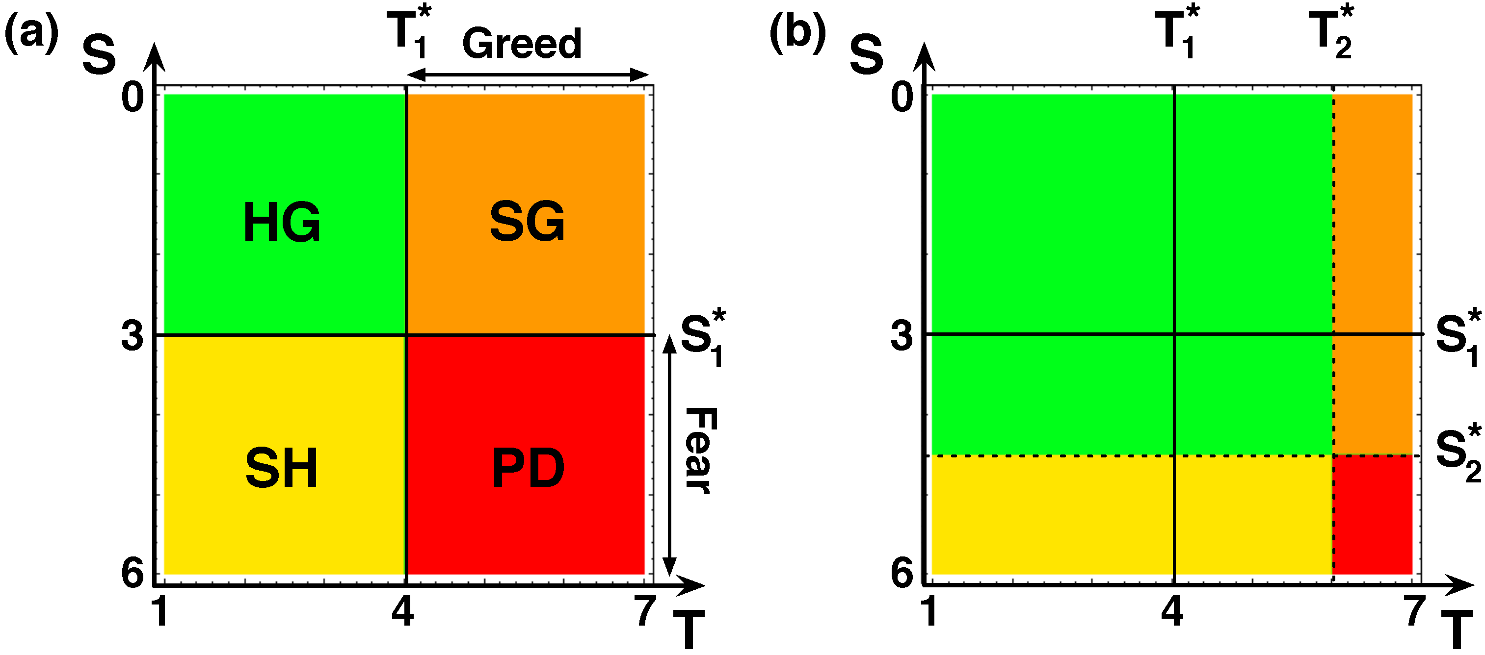
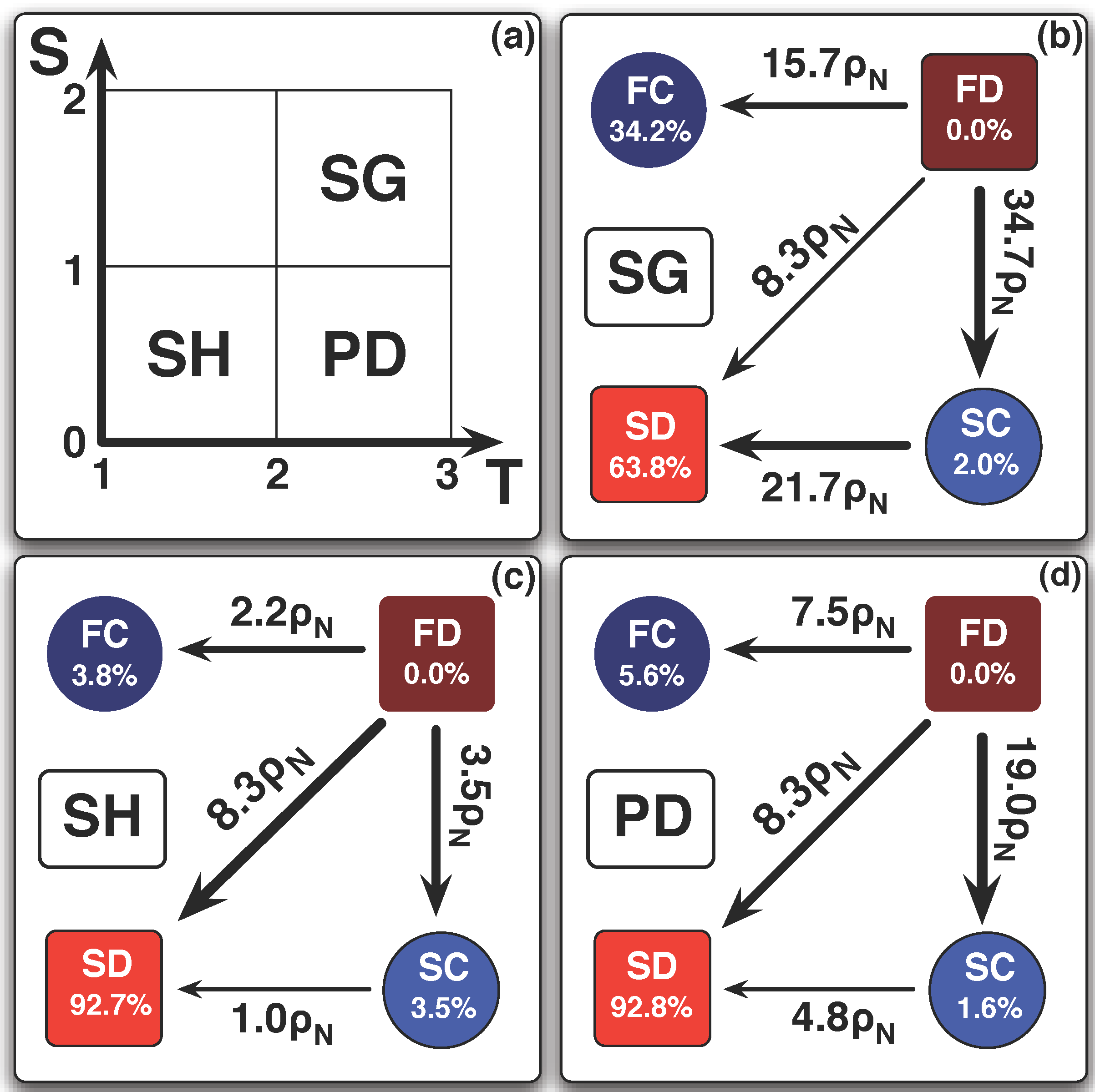
• Coordination or Bistability: $T<R$ and $S<P$ leads to what is called coordination or SH games [65], in which it is always beneficial to follow the strategy of the opponent, turning both C’s and D’s advantageous when rare.
• Coexistence: In the case of $R<T$ and $P<S$, known as the SG [66,67,68], a small minority of C’s or D’s is always favored. This means that the ultimate outcome in a population of players is a mixture of C’s and D’s.

When mutual cooperation R is preferred to mutual defection P, the 2-D parameter space defined by T and S characterizes all three scenarios introduced above, as illustrated in Figure 1(a), using $R=4$ and $P=3$. Two critical payoff values, $T_1^{*}$ and $S_1^{*}$, mark the boundaries of the regions associated with the different types of games. When $T>T_1^{*}=R$, joint cooperation is threatened by greed: the temptation to defect towards a cooperator. Similarly, when $S<S_1^{*}=P$, joint cooperation is threatened by the fear of being betrayed by a defector [36,70].

Within the context of these social scenarios, two dynamical processes take place in the population simultaneously: evolution of individual (game) behavior on the one hand, and evolution of the network structure on the other hand. Each of these two processes proceeds on a characteristic time scale: ${\tau }_a$ denotes the time scale associated with network evolution, ${\tau }_s$ denotes the one associated with behavior (strategy) evolution. The next two subsections explain in detail each of these two processes.

Figure 1. Game transformation through AL. (a) 2-D parameter space, defined by T and S, characterizing four games: HG, SH, SG and PD ($R=4$ and $P=3$). The critical game parameters $T_1^{*}$ and $S_1^{*}$ separate the different regions. Greed comes into play when $T>T_1^{*}$, fear when $S<S_1^{*}$. (b) AL changes the nature of the game being played. Even though individuals engage in the same game, greed (fear) will come into play only when $T>T_2^{*}$ ($S<S_2^{*}$). $T_2^{*}$ and $S_2^{*}$ were calculated using $c=0.16$, ${\gamma }_{CC}=0.16$, ${\gamma }_{CD}=0.8$, ${\gamma }_{DD}=0.32$.

Figure 1. Game transformation through AL. (a) 2-D parameter space, defined by T and S, characterizing four games: HG, SH, SG and PD ($R=4$ and $P=3$). The critical game parameters $T_1^{*}$ and $S_1^{*}$ separate the different regions. Greed comes into play when $T>T_1^{*}$, fear when $S<S_1^{*}$. (b) AL changes the nature of the game being played. Even though individuals engage in the same game, greed (fear) will come into play only when $T>T_2^{*}$ ($S<S_2^{*}$). $T_2^{*}$ and $S_2^{*}$ were calculated using $c=0.16$, ${\gamma }_{CC}=0.16$, ${\gamma }_{CD}=0.8$, ${\gamma }_{DD}=0.32$.

2.1. Network Evolution

Individuals can decide to establish new connections and to remove existing ones, making the number of edges a variable quantity which changes in time. New edges appear randomly at a fixed rate c and have characteristic life-times. In this section, we assume that the lifetime of a link depends solely on the game behavior of the individuals involved. Specifically, the rate at which CC, CD and DD links disappear is given by ${\gamma }_{CC}$, ${\gamma }_{CD}$ and ${\gamma }_{DD}$, respectively. The next sections incorporate additional realism by assigning each individual a characteristic eagerness to break nonproductive connections. In real populations, the likelihood for edges to appear or disappear may depend on other factors, not dealt with in this work, such as the geographical distance between individuals, the existence of family relationships or the social context wherein individuals find themselves. Individual-based linking rules are required to capture such a melting pot of influences, implying the use of computer simulations to study the population’s evolution (see e.g., [49,50,51,54,55,56,57,59,60,61,63]). The linking rules considered in the present work, on the other hand, allow us to describe the network dynamics using the following set of ordinary differential equations

$$\begin{array}{c}\hfill {\dot{L}}_{ij}\left(t\right)=c\left[N_{ij}\left(t\right)-L_{ij}\left(t\right)\right]-{\gamma }_{ij}{L}_{ij}\left(t\right)\end{array}$$

(2)

$L_{ij}\left(t\right)$ stands for the number links between individuals with strategy i and individuals with strategy j at time t. $N_{ij}\left(t\right)$ is the maximum possible number of such links. This maximum depends on the number of i and j individuals in the population, which we denote by $N_i\left(t\right)$ and $N_j\left(t\right)$, respectively, and equals

$$N_{ij}\left(t\right)=\left\{\begin{array}{cc}\hfill N_i\left(t\right)N_j\left(t\right)& (i\ne j)\hfill \\ \hfill \frac{1}{2}{N}_i\left(t\right)[N_i\left(t\right)-1]& (i=j)\hfill \end{array}\right.$$

Whenever the strategies of the individuals remain fixed for a sufficiently long time (see time scale discussion below), the network will evolve towards a steady state with single-scale to broad-scale heterogeneity [52,71] and a stationary number of links of each type given by

$$\begin{array}{c}\hfill L_{ij}^{*}={\varphi }_{ij}{N}_{ij}\end{array}$$

(3)

where ${\varphi }_{ij}=c{(c+{\gamma }_{ij})}^{-1}$. Note that $L_{ij}^{*}$ depends on the actual strategy configuration of the population, illustrating the coupling between network dynamics and strategy dynamics. Examples of population structures attained under steady-state dynamics for three different combinations of ($N_C,N-N_C$) are shown in Figure 2.

Figure 2. Frequency-dependent network evolution. Blue circles indicate C’s, red circles indicate D’s. CC-links are depicted as cyan lines, CD-links as red lines and DD-links as gray lines. Each panel shows a snapshot of a network in the steady state of the network dynamics associated with given configuration of C’s and D’s. The parameters governing the network dynamics are $c=0.25,{\gamma }_{CC}=0.5,{\gamma }_{CD}=0.25$ and ${\gamma }_{DD}=0.5$. The total population size is $N=30$. Figure reproduced from [53].

Figure 2. Frequency-dependent network evolution. Blue circles indicate C’s, red circles indicate D’s. CC-links are depicted as cyan lines, CD-links as red lines and DD-links as gray lines. Each panel shows a snapshot of a network in the steady state of the network dynamics associated with given configuration of C’s and D’s. The parameters governing the network dynamics are $c=0.25,{\gamma }_{CC}=0.5,{\gamma }_{CD}=0.25$ and ${\gamma }_{DD}=0.5$. The total population size is $N=30$. Figure reproduced from [53].

2.2. Strategy Evolution

In this section, we assume that individuals adjust their strategy solely by imitating others, which means that they can only adopt strategies that are already present in the population. As of Section 3, we will use an extended version of this strategy update rule and give individuals the opportunity to try out completely new strategies occasionally (see Section 3.1). The imitation process itself is defined according to the pairwise-comparison rule [23,72,73]. At every strategy update event, a focal individual X is selected randomly from the population. This individual adopts the strategy of a random individual Y—his role model—with probability

$$\begin{array}{c}\hfill p_{XY}={\left[1+e^{\beta ({\Pi }_X-{\Pi }_Y)}\right]}^{-1}\end{array}$$

(4)

${\Pi }_X$ (${\Pi }_Y$) denotes the total payoff X (Y) receives after interacting once with every neighbor. The parameter β ($\ge 0$) controls the intensity of selection and measures the importance of game payoff in the imitation process. In the limit $\beta \to \infty$, individuals imitate each other based purely on the payoffs they acquire. The game becomes progressively less important for decreasing β. In the limit $\beta \to 0$, strategies evolve in a purely random fashion, according to the same rules as those of the so-called voter model [74]. The imitation process defined above assumes that all individuals are equally likely to act as each other’s role model, whereas it is now well-known that cooperation is maximized whenever individuals are limited to imitate those with whom they interact [75,76]. In this sense, the levels of cooperation reported in the present work can be considered as pessimistic estimates of the actual levels.

Note that the strategy dynamics can be represented as a Markov Chain (MC) [11,77]. Each state of the MC corresponds to a certain strategy configuration of the population. The population moves from one state to the next as individuals adjust their behavior. As long as the dynamics proceeds stochastically, i.e., when β is finite, the population will eventually end up in a homogeneous state (all individuals adopting the same strategy). Below, we discuss how AL affects the probability to reach each of these states.

2.3. Separation of Time Scales

The impact of the network dynamics on the strategy dynamics depends on the ratio $W=\frac{{\tau }_s}{{\tau }_a}$. There are two limiting cases: fast strategy dynamics ($W\ll 1$) and fast linking dynamics ($W\gg 1$).

In case of fast strategy dynamics, the network changes so slowly that strategies evolve as on a static network. The network topology, which corresponds to an initial condition in our case, complicates the analytical treatment of the system. Analytical solutions are feasible only for few topologies, in the limit of weak selection ($\beta \to 0$) [37,78]. Complete networks, corresponding to well-mixed systems, are the simplest type of networks. In such networks, we can calculate analytically the probability ${\rho }_{N_C}$ that a population of $N_C$ C’s evolves towards full cooperation. This probability can be approximated by [72]

$${\rho }_{N_C}\approx \frac{\mathrm{erf}\left[{\xi }_{N_C}\right]-\mathrm{erf}\left[{\xi }_0\right]}{\mathrm{erf}\left[{\xi }_N\right]-\mathrm{erf}\left[{\xi }_0\right]}$$

(5)

where $\mathrm{erf}\left(x\right)$ is the error function and ${\xi }_k=\sqrt{\frac{\beta }{u}}(ku+v)$. We have $2u=R-S-T+P$ and $2v=-R+SN-TN+T$.

In case of fast linking dynamics, strategy update events do not occur before the network has reached its stationary configuration. The average fitness of C’s and D’s during a strategy update event is therefore given by

$$\begin{array}{cc}\hfill {\Pi }_C^{*}=& R{\varphi }_{CC}(N_C-1)+S{\varphi }_{CD}(N-N_C)\hfill \\ \hfill {\Pi }_D^{*}=& T{\varphi }_{CD}{N}_C+P{\varphi }_{DD}(N-N_C-1)\hfill \end{array}$$

(6)

Note that these payoff values correspond to those obtained in a complete network with the same strategy configuration, but using the following rescaled payoff matrix

$$M^{\prime }=\begin{array}{cc}& \begin{array}{cc}C& D\end{array}\\ \begin{array}{c}C\\ D\end{array}& \left(\begin{array}{cc}{R}^{\prime }& S^{\prime }\\ T^{\prime }& P^{\prime }\end{array}\right)\end{array}=\left(\begin{array}{cc}R{\varphi }_{CC}& S{\varphi }_{CD}\\ T{\varphi }_{CD}& P{\varphi }_{DD}\end{array}\right)$$

(7)

Consequently, network evolution can change the nature of the game. Even though individuals engage in a game characterized by payoff matrix M, their behavior will evolve like in a complete network, but using payoff matrix $M^{\prime }$. Naturally, this game transformation changes the critical payoff values $T_1^{*}$ and $S_1^{*}$ to $T_2^{*}$ and $S_2^{*}$. These new values are given by

$$T_2^{*}=R\frac{{\varphi }_{CC}}{{\varphi }_{CD}}=R\frac{c+{\gamma }_{CD}}{c+{\gamma }_{CC}}$$

(8)

and

$$S_2^{*}=P\frac{{\varphi }_{DD}}{{\varphi }_{CD}}=P\frac{c+{\gamma }_{CD}}{c+{\gamma }_{DD}}$$

(9)

Figure 1(b) illustrates the game transformation resulting from AL for ${\gamma }_{CC}=0.16$, ${\gamma }_{CD}=0.80$, ${\gamma }_{DD}=0.32$. It is clear, for instance, that the PD region reduces significantly in favor of games that are more favorable to cooperation.

2.4. Comparable Time Scales

As we have shown, AL can lead to a wide range of scenarios that effectively change the character of the game. However, the analytical results have been obtained under the assumption that the network evolves much faster than the individual strategies do. As this may not always be the case, it is important to assess the domain of validity of this limit.

Figure 3 shows the probability, calculated using numerical simulations, that the population fixates into full cooperation, and this as a function of the time scale ratio W. Each simulation starts with a complete network of size $N=100$, containing $50\%$ C’s and $50\%$ D’s, who interact in a PD specified by the following payoff matrix

$$\begin{array}{cc}& \begin{array}{cc}C& D\end{array}\\ \begin{array}{c}C\\ D\end{array}& \left(\begin{array}{cc}4& 2\\ 5& 3\end{array}\right)\end{array}$$

(10)

Strategy evolution and network evolution proceed together under asynchronous updating. Strategy update events take place with probability $\frac{1}{1+W}$, while network update events occur with probability $\frac{W}{1+W}$. We run each simulation until fixation, i.e., until we obtain full cooperation or full defection, and plot the resulting probabilities as a function of W.

The following parameters specify the network dynamics: $c=0.16$, ${\gamma }_{CC}=0.16$, ${\gamma }_{CD}=0.80$ and ${\gamma }_{DD}=0.32$. In the fast linking limit, the individuals behave as if they were playing the following game in a complete network (see Equation 7):

$$\begin{array}{cc}& \begin{array}{cc}C& D\end{array}\\ \begin{array}{c}C\\ D\end{array}& \left(\begin{array}{cc}2& \frac{1}{3}\\ \frac{5}{6}& 1\end{array}\right)\end{array}$$

(11)

This game is no longer a PD, but a SH. With $W\gg 1$ and an initial fraction of $50\%$ C’s, the population should always evolve towards full cooperation. However, Figure 3 indicates that the population reaches full cooperation for a much wider range of time scales. For the extreme limits we obtain a perfect agreement with the analytical results, whereas deviations from the analytical predictions are limited to a single order of magnitude. In other words, the time scale separation is not a very strong assumption and remains valid for a much wider range of parameters than expected. Even for moderate active linking, the analytical results are recovered.

Figure 3. AL changes the nature of the game, even outside the time scale separation limit. We start from $50\%$ cooperating individuals. For small W, C’s never reach fixation. But already for $W=0.1$, fixation of C’s is almost certain. Thus, moderate AL is sufficient to turn cooperation into the dominant strategy here. Results are averages over 100 realizations. ($N=100$, $\beta =0.05$, $c=0.16$, ${\gamma }_{CC}=0.16$, ${\gamma }_{CD}=0.80$ and ${\gamma }_{DD}=0.32$). Figure reproduced from [52].

Figure 3. AL changes the nature of the game, even outside the time scale separation limit. We start from $50\%$ cooperating individuals. For small W, C’s never reach fixation. But already for $W=0.1$, fixation of C’s is almost certain. Thus, moderate AL is sufficient to turn cooperation into the dominant strategy here. Results are averages over 100 realizations. ($N=100$, $\beta =0.05$, $c=0.16$, ${\gamma }_{CC}=0.16$, ${\gamma }_{CD}=0.80$ and ${\gamma }_{DD}=0.32$). Figure reproduced from [52].

3. Diversity and Cooperation in the PD

The previous section introduced AL for the simple case in which there are only three possible break-up rates for links: ${\gamma }_{CC}$, ${\gamma }_{CD}$ and ${\gamma }_{DD}$. In the following, we assign each individual explicitly a linking strategy, which determines how to manage different social contacts. Up to now, this linking strategy was dependent solely on the game strategy of the individual. This situation contrasts with our everyday experience where we recognize a more continuous behavioral spectrum. Even when two individuals cooperate, their decision to remove links can be completely different. Take as an example the inherent tendency of people to have an aversion for risks [79].

As such, we define an individual’s strategy as a pair, combining both game behavior and linking behavior. This section discusses how the presence of behavioral differences at the level the linking strategy of the individuals affects the overall chances of cooperators in the PD.

3.1. A Minimal Model

Let us stick to C’s and D’s, engaging in a one-shot, symmetric, two-player PD game as defined by Payoff matrix 1, with $S<R$ and $P<T$. Irrespective of one’s game strategy (C or D), interacting with a C always leads to a higher payoff than interacting with a D. Individuals will therefore be satisfied about their connections with C’s and would like to maintain these as long as possible. Connections with D’s, on the other hand, can be considered as adverse and will be broken at different rates, determined by the individuals’ linking strategy. We introduce behavioral diversity by considering M (usually many) different linking strategies, and study the entangled co-evolution of game strategy and linking strategy with the self-organization of the population structure.

Let us denote the combined game and linking strategies as $S_i$, with i∈$\{1,\cdots ,2M\}$. The rate at which new interactions appear is fixed and independent of the game or linking strategies of the individuals involved. As in the previous section, we use c to denote this rate. Links connecting $S_i$ individuals with $S_j$ individuals disappear at rate ${\kappa }_{ij}=\frac{1}{2}({\gamma }_{ij}+{\gamma }_{ji})$, where ${\gamma }_{ij}^{-1}$ (${\gamma }_{ji}^{-1}$) is the average time $S_i$ ($S_j$) individuals would attribute to links with $S_j$ ($S_i$) individuals. The value ${\gamma }_{ij}$ reflects whether $S_i$ individuals are satisfied or dissatisfied with their links with $S_j$ individuals. When satisfied, ${\gamma }_{ij}$ is taken as the minimum value γ among all ${\gamma }_{ij}$. When dissatisfied, on the other hand, ${\gamma }_{ij}$ is given by the linking strategy of $S_i$ individuals and satisfies ${\gamma }_{ij}\ge \gamma$. The corresponding linking dynamics of the network can be described by ordinary differential equations analogous to those in Equation 2, leading to a certain equilibrium distribution of links (see Equation 3).

Strategies spread in the population according to a mutation-selection process defined by the pairwise-comparison rule [23,72] (see Section 2.2). At every strategy update, an individual X is drawn randomly from the population. With probability μ, he adopts a strategy selected randomly from all $2M$ available strategies. Otherwise, we select a random individual Y, who will be imitated by X with probability $p_{XY}$ (see Equation 4).

In the limit of fast linking ($W\gg 1$), the fitness of an $S_i$ individual is given by:

$$f_i=\sum _j{a}_{ij}{\varphi }_{ij}(N_j-{\delta }_{ij})$$

(12)

where $A={\left[a_{ij}\right]}_{i,j=1,\cdots ,2M}$ is the game payoff matrix, $N_j$ the number of $S_j$ individuals and ${\delta }_{ij}$ is Kronecker delta. This is mathematically equivalent to the fitness of an $S_i$ individual playing a game specified by the rescaled payoff matrix

$$B={\left[b_{ij}\right]}_{i,j=1,\cdots ,2M}={\left[a_{ij}{\varphi }_{ij}\right]}_{i,j=1,\cdots ,2M}$$

(13)

in a complete network (see Equation 7). Thanks to this mapping with complete networks, it is possible to compute analytically the (fixation) probability ${\rho }_{ij}$ that an individual with strategy $S_i$ takes over a population of $N-1$ individuals with strategy $S_j$ (see Equation 5), assuming that meanwhile no additional strategies appear because of mutations. Note that it is no longer possible to describe the overall population behavior in terms of one game only, like in the previous section. The wide range of different linking strategies leads to a multi-dilemma environment. Although all individuals engage in the same game, they may perceive that game differently, depending on their linking strategy.

As we address the role of behavioral diversity in this work, we will typically consider more than two possible strategies ($M>1$), which precludes an analytical description of the stochastic evolutionary dynamics for arbitrary mutation rates. By assuming that mutations rarely occur (when compared with strategy update events), we can analytically describe the system in a compact form [80,81]. The evolutionary dynamics does no longer proceed in the entire $2M$-dimensional strategy space, but only along its boundaries [80,81], where there are never more than two different strategies present simultaneously. Indeed, as long as no mutations occur, stochastic update dynamics always drives the population to a homogeneous state (monomorphic population), i.e., a state in which only individuals of one particular strategy survive. Assuming a monomorphic population, a specific new strategy will show up with probability $\frac{\mu }{2M-1}$ and to the extent that μ is sufficiently small, this mutant will go extinct or will fixate before any new mutation occurs. We can approximate this system by a Markov Chain with only $2M$ states, each state corresponding to a certain homogeneous state of the population. The probability that the appearance of a random mutant in a state with otherwise only $S_i$ individuals moves the population to a state with only $S_j$ individuals defines the transition probability between the corresponding states of the Markov Chain. These probabilities define the transition matrix Λ of the Markov Chain, which is given by $\Lambda ={\left[{\Lambda }_{ij}\right]}_{i,j=1,\cdots ,2M}$, where ${\Lambda }_{ii}=1-\frac{1}{2M-1}{\sum }_{k=1,k\ne i}^{2M}{\rho }_{ki}$ and ${\Lambda }_{ij}=\frac{{\rho }_{ji}}{2M-1}$ ($j\ne i$). The normalized left eigenvector of the unit eigenvalue of Λ defines the stationary distribution, i.e., the fraction of time the population spends in each of the available strategies. The stationary distributions obtained using this small-mutation approach also hold for larger mutation rates, as also shown in [81].

3.2. Two Linking Strategies

The most simple configuration is the one in which there are only two different linking strategies ($M=2$): Individuals break up adverse connections either at a slow rate ${\gamma }_S$, or at a fast rate ${\gamma }_F$. In combination with the game strategy we obtain a total of four different strategies: slow C’s (SC’s) and D’s (SD’s), whose adverse interactions last long, and fast C’s (FC’s) and D’s (FD’s), whose adverse interactions are short lived. Following Equation 7, we obtain the payoff matrix:

$$\begin{array}{cc}& \begin{array}{cccc}SC& FC& SD& FD\end{array}\\ \begin{array}{c}SC\\ FC\\ SD\\ FD\end{array}& \left(\begin{array}{cccc}R{\varphi }_S& R{\varphi }_S& S{\varphi }_S& S{\varphi }_S\\ R{\varphi }_S& R{\varphi }_S& S{\varphi }_M& S{\varphi }_M\\ T{\varphi }_S& T{\varphi }_M& P{\varphi }_S& P{\varphi }_M\\ T{\varphi }_S& T{\varphi }_M& P{\varphi }_M& P{\varphi }_F\end{array}\right)\end{array}$$

(14)

where ${\varphi }_x=c{(c+{\kappa }_x)}^{-1}$, with ${\kappa }_S={\gamma }_S$, ${\kappa }_M=\frac{1}{2}({\gamma }_S+{\gamma }_F)$ and ${\kappa }_F={\gamma }_F$.

Adopting the small-mutation approach discussed above, the complex co-evolutionary dynamics reduces to one associated with a Markov Chain with only 4 ($2M$) states. The Markov Chain’s transitions that are favored by natural selection, i.e., those that are larger than ${\rho }_N=\frac{1}{N}$ (the fixation probability associated with neutral evolution), characterize the main driving forces of the evolutionary dynamics. These transitions are shown in Figure 4 for a region where D’s dominate. The exact values are obtained by computing the probability that a mutant (with strategy located at the end of each arrow) fixates in a monomorphic population of individuals adopting the strategy located at the start of the arrow. We see that SD’s are clearly the winners of the evolutionary race. FD’s, on the other hand, are rendered disadvantageous with respect to any other strategy. When a FC manages to fixate, we end up in a rather stable scenario. In addition, SC’s acquire a transient character, providing an alternative route from FD to SD. In this specific case, it is, however, mainly the direct transition from FD’s into SD’s that hinders C’s survivability. As we will show below, the viability of C’s relies on the extent to which the transition FD → SD is inhibited compared to transitions into FC’s.

Figure 4. Transition probabilities and stationary distributions for a population with $M=2$ different linking strategies. In the limit of rare mutations, the dynamics reduces to transitions between homogeneous states of the population [80,81]. The arrows indicate those transitions for which the fixation probability is greater than neutral fixation, ${\rho }_N=\frac{1}{N}$. The explicit values were obtained analytically with the pairwise comparison rule (see Equation 5). Adaptive network dynamics allows C’s, in the form of SC or FC, to remain in the population for $7.2\%$ of the time. D’s dominate because of the flow from FD to SD, either directly or by using the alternative route via SC. (N = 100, β = 0.01, T = 2.1, R = 2, S = 0.9, P = 1, c = 0.16, δ = 0.3). Figure reproduced from [62].

Figure 4. Transition probabilities and stationary distributions for a population with $M=2$ different linking strategies. In the limit of rare mutations, the dynamics reduces to transitions between homogeneous states of the population [80,81]. The arrows indicate those transitions for which the fixation probability is greater than neutral fixation, ${\rho }_N=\frac{1}{N}$. The explicit values were obtained analytically with the pairwise comparison rule (see Equation 5). Adaptive network dynamics allows C’s, in the form of SC or FC, to remain in the population for $7.2\%$ of the time. D’s dominate because of the flow from FD to SD, either directly or by using the alternative route via SC. (N = 100, β = 0.01, T = 2.1, R = 2, S = 0.9, P = 1, c = 0.16, δ = 0.3). Figure reproduced from [62].

3.3. Arbitrary Number of Linking Strategies

We now extend the analysis to an arbitrary number of linking strategies M, with rates for breaking adverse ties taken uniformly in the interval $[0.5-\delta ,0.5+\delta ]$. This leads to a trivial generalization of Matrix 14. Figure 5(a) shows that cooperation blooms when the number of linking strategies M increases. In the following, we investigate the mechanism responsible for this remarkable performance of C’s.

A first hint is provided in Figure 5(b), where the fraction of time spent in each state of the population is shown for the case in which there are $M=50$ possible types (linking strategies). We see that all types of C’s are present in the population, whereas the D’s who survive are only of the slowest types. Importantly, however, with increasing number of available types, the difference between the values of the rates associated with contiguous types is reduced, which provides a means for D’s other than the slowest to survive in the population. These are precisely the D’s who provide an escape hatch for C’s to survive (cf. Figure 4), since many of them will be disadvantageous with respect to C’s. Indeed, Figure 5(b) shows that increasing the number of possible types, D’s with break-up rates higher than the minimum γ are now able to survive. Although these individuals do not dominate, they effectively promote the appearance of fast C’s, since the transition $D\to C$ between these types is favored by natural selection. On the other hand, because all C-types are neutral with respect to each other, they end up fairly equally distributed in the population, unlike D’s for whom natural selection favors the slower types (cf. Figure 5(b). Figure 6(b) also shows that, with increasing number of types, the number of C-types which are favored increases more than the corresponding number of D-types. As a result, all but the slowest D’s are disadvantageous with respect to (most of the) C’s. Increasing the number of types efficiently inhibits the transition from the fastest to the slowest D’s, paving the way for cooperation to thrive, an effect which remains valid irrespective of the model parameters, inasmuch as T and S are such that cooperators manage to survive. Mathematically, a large number of different types allows individuals to engage in a wider range of games and the complex set of different interactions allows the appearance of D’s from which C’s can profit.

Figure 5. Cooperation and behavioral diversity. (a) The population spends more time in a cooperative state (of any type) when the number of possible types (M) increases, irrespective of the temptation to defect T in the PD. (N=100, β=0.1, c=0.16, δ=0.3$,R$=2, P=1, S=$3-T$) (b) While the majority of cooperator types is equally represented, only the slower types of defectors manage to survive. The defector population exhibits behavioral differences, which inhibits the dominance of slowest defector type, providing an escape hatch for cooperation to thrive (M=50, T=2.1, R=2, P=1, S=0.9). Figure reproduced from [62].

Figure 5. Cooperation and behavioral diversity. (a) The population spends more time in a cooperative state (of any type) when the number of possible types (M) increases, irrespective of the temptation to defect T in the PD. (N=100, β=0.1, c=0.16, δ=0.3$,R$=2, P=1, S=$3-T$) (b) While the majority of cooperator types is equally represented, only the slower types of defectors manage to survive. The defector population exhibits behavioral differences, which inhibits the dominance of slowest defector type, providing an escape hatch for cooperation to thrive (M=50, T=2.1, R=2, P=1, S=0.9). Figure reproduced from [62].

4. Selection Pressure and Behavioral Diversity

No two populations are the same. While behavioral differences among individuals are substantial in some populations, we observe a much more uniform behavioral pattern in others. Moreover, in some populations one recognizes a higher sensitivity to behavioral differences than in others. Here we adopt the model proposed in the previous section and investigate analytically how changes in the range of the behavioral spectrum (δ) and in the selection pressure (β) affect the evolution of cooperation.

Figure 7 shows , for the PD, the fraction of time the population spends in a cooperative state (of any type) as a function of δ and β. The number of types is chosen in such a way that the distance d between the rates of every two consecutive types remains constant (equal to 0.01 in this case). The figure shows that for each value of δ there exists and interval of β that maximizes cooperation. Whenever the selection pressure is very high (large β, corresponding to pure imitation dynamics) only the slowest D’s survive. Consequently, they outcompete C’s, irrespective of the number of possible types. δ plays a role for intermediate regimes of selection pressure, in which cooperation increases with increasing δ. Finally, as selection becomes very weak ($\beta \ll 1$), drift dominates selection and behavioral differences become progressively irrelevant.

Figure 6. Transition probabilities and stationary distributions for the PD game with $M=3$ (a) and $M=10$ (b) types of individuals. The population spends already $59.8\%$ of the time in a cooperative state when $M=10$. Numbering C’s and D’s according to their type, C0 (D0) being the slowest cooperator (defector), we see that increasing M splits the “outflow” of fast defectors among a wide range of different possibilities. As a result, cooperation emerges, since only few types of defectors are evolutionarily stable, whereas the vast majority of cooperative types work as “flow sinks”. ($N=100$, $T=2.1$, $R=2$, $S=0.9$, $P=1$, $c=0.16$, $\beta =0.01$, $\delta =0.3$). Figure reproduced from [62].

Figure 6. Transition probabilities and stationary distributions for the PD game with $M=3$ (a) and $M=10$ (b) types of individuals. The population spends already $59.8\%$ of the time in a cooperative state when $M=10$. Numbering C’s and D’s according to their type, C0 (D0) being the slowest cooperator (defector), we see that increasing M splits the “outflow” of fast defectors among a wide range of different possibilities. As a result, cooperation emerges, since only few types of defectors are evolutionarily stable, whereas the vast majority of cooperative types work as “flow sinks”. ($N=100$, $T=2.1$, $R=2$, $S=0.9$, $P=1$, $c=0.16$, $\beta =0.01$, $\delta =0.3$). Figure reproduced from [62].

Figure 7. Role of the range of behavioral spectrum (δ) and selection pressure (β) in the evolution of cooperation. Each contour region represents the fraction of time the population spends in a cooperative state (of any type), for given values of δ and β. The number of types in the population was changed so as to keep the interval in δ between consecutive types constant (0.01). Specifically, $\delta =0.3$ leads to 60 types in the population. ($N=100,T=2.1,R=2,P=1,S=0.9,c=0.16$).

Figure 7. Role of the range of behavioral spectrum (δ) and selection pressure (β) in the evolution of cooperation. Each contour region represents the fraction of time the population spends in a cooperative state (of any type), for given values of δ and β. The number of types in the population was changed so as to keep the interval in δ between consecutive types constant (0.01). Specifically, $\delta =0.3$ leads to 60 types in the population. ($N=100,T=2.1,R=2,P=1,S=0.9,c=0.16$).

Overall, the message is clear: Inasmuch as C’s have a chance, the presence of a wide range of different social preferences favors cooperation. This is also the case when one varies the distance between the rates of consecutive types, as shown in Figure 8.

Figure 8. Role of separation d between consecutive rates in the evolutionary success of cooperators. The plots shows the fraction of time the population spends in a cooperative state (of any type) for a given intensity of selection. Symbols represent the data. The lines are the result of a spline interpolation of the data. Each data set corresponds to a different distance d between consecutive rates (and types) in the population. Smaller values of d lead to more cooperation, an effect that becomes more pronounced for intermediate intensities of selection. In these regimes, small distances between types can effectively reduce the “flow” towards the slowest defector type, as discussed in Section 3. ($N=100,T=2.1,R=2,P=1,S=0.9,c=0.16,\delta =0.3$).

Figure 8. Role of separation d between consecutive rates in the evolutionary success of cooperators. The plots shows the fraction of time the population spends in a cooperative state (of any type) for a given intensity of selection. Symbols represent the data. The lines are the result of a spline interpolation of the data. Each data set corresponds to a different distance d between consecutive rates (and types) in the population. Smaller values of d lead to more cooperation, an effect that becomes more pronounced for intermediate intensities of selection. In these regimes, small distances between types can effectively reduce the “flow” towards the slowest defector type, as discussed in Section 3. ($N=100,T=2.1,R=2,P=1,S=0.9,c=0.16,\delta =0.3$).

The smaller the separation between the rates of consecutive types, the better for cooperation, a feature which is most pronounced for selection pressures at which D’s start to outcompete C’s. Clearly, increasing the number of possible types is always beneficial to cooperation, as in this way it is most inefficient for D’s to transform into their most fit type, and then outcompete C’s.

5. Diversity and Cooperation in the Snowdrift and Stag-hunt games

In Section 3 we studied the effect of differences in responsiveness to adverse social ties for individuals engaging in the PD game. Here we extend the analysis to the other two-player dilemmas of cooperation: the SH and SG.

We by analyzing the simplest case in which we have only two types of C’s and D’s. Figure 9 depicts the transition probabilities and stationary distributions for both SG and SH, in addition to the previously analyzed PD. It is clear that the three dilemmas portray, qualitatively, the same scenario.

Fast D’s are easily wiped out by any other possible behavior. At the same time $FD$ provides a route towards the emergence of fast C’s, a strategy that is very well protected against invasion by D’s. Yet, the population remains most of the time in the $SD$ strategy, inhibiting $FD$ from playing its role as a catalyzer of cooperation.

Figure 9. Transition probabilities and stationary distributions for the stag-hunt and snowdrift games. (a) Two-dimensional parameter space defining all three social dilemmas. By fixing $R=2$ and $P=1$, while $0\le S\le 1$ and $1\le T\le 3$, we can represent the three most popular social dilemmas of cooperation: The PD ($S<1$ and $T>2$), the SG ($S>1$ and $T>2$) and the SH ($S<1$ and $T<2$). (b), (c) and (d) Transition probabilities and stationary distributions for the three dilemmas with two types of individuals. The dynamics is reduced to transitions between homogeneous states of the population. The arrows in black indicate those transitions for which the fixation probability ρ is greater than neutral fixation (${\rho }_N=\frac{1}{N}$). The explicit values are calculated using the pairwise comparison rule with parameters $N=100$, $\beta =0.01$, $c=0.16$ and $\delta =0.3$. The examples shown were obtained for $T=2.1$, $S=0.9$ (PD), $T=2.65$, $S=1.35$ (SG) and $T=1.65$, $S=0.35$ (SH).

Figure 9. Transition probabilities and stationary distributions for the stag-hunt and snowdrift games. (a) Two-dimensional parameter space defining all three social dilemmas. By fixing $R=2$ and $P=1$, while $0\le S\le 1$ and $1\le T\le 3$, we can represent the three most popular social dilemmas of cooperation: The PD ($S<1$ and $T>2$), the SG ($S>1$ and $T>2$) and the SH ($S<1$ and $T<2$). (b), (c) and (d) Transition probabilities and stationary distributions for the three dilemmas with two types of individuals. The dynamics is reduced to transitions between homogeneous states of the population. The arrows in black indicate those transitions for which the fixation probability ρ is greater than neutral fixation (${\rho }_N=\frac{1}{N}$). The explicit values are calculated using the pairwise comparison rule with parameters $N=100$, $\beta =0.01$, $c=0.16$ and $\delta =0.3$. The examples shown were obtained for $T=2.1$, $S=0.9$ (PD), $T=2.65$, $S=1.35$ (SG) and $T=1.65$, $S=0.35$ (SH).

For all dilemmas, when the number of types increases, not only the slowest D’s survive, but also other D’s who are slightly faster (see Figure 10). This, as explained before, opens a route for the fixation of fast C’s enhancing the overall survival of cooperation. Irrespective of the dilemma at stake, cooperation profits from the presence of individuals that respond differently to unwanted partners, which evidences the general validity of the present results.

Figure 10. Impact of behavioral differences on cooperation in the snowdrift (upper panels) and stag-hunt (lower panels) games. The plots on the left depict the fraction of time the population spends in a cooperative state (of any type) as a function of the number of types M in the population. Each line corresponds to a different value of the temptation to defect T ($R=2$, $P=1$, $S=4-T$ for the SG and $S=2-T$ for the SH). Irrespective of T, cooperation increases with increasing number of types. The bar plots on the right ($T=2.65$ and $S=1.35$ for the SG and $T=1.65$, $S=0.35$ for the SH game), depict the fraction of time that each type of individual is present in a population with 50 different types. While all types of C’s survive, only the slower types of D’s remain in the population. However, the surviving D’s exhibit heterogeneity. As faster D’s manage to survive, part of the strategy flow is diverted into fast C’s ($N=100$, $\beta =0.01$, $M=50$, $c=0.16$ and $\delta =0.3$).

Figure 10. Impact of behavioral differences on cooperation in the snowdrift (upper panels) and stag-hunt (lower panels) games. The plots on the left depict the fraction of time the population spends in a cooperative state (of any type) as a function of the number of types M in the population. Each line corresponds to a different value of the temptation to defect T ($R=2$, $P=1$, $S=4-T$ for the SG and $S=2-T$ for the SH). Irrespective of T, cooperation increases with increasing number of types. The bar plots on the right ($T=2.65$ and $S=1.35$ for the SG and $T=1.65$, $S=0.35$ for the SH game), depict the fraction of time that each type of individual is present in a population with 50 different types. While all types of C’s survive, only the slower types of D’s remain in the population. However, the surviving D’s exhibit heterogeneity. As faster D’s manage to survive, part of the strategy flow is diverted into fast C’s ($N=100$, $\beta =0.01$, $M=50$, $c=0.16$ and $\delta =0.3$).

6. Conclusions

The first part of this article provides an extensive review of the AL framework in the context of 2-person social dilemmas. The second part uses this framework to address the consequences of individual diversity in treating adverse social contacts, a feature which is omnipresent in real-world social systems but mostly neglected in theoretical studies on cooperation. The present work shows that such diversity provides a perfect breeding ground for cooperation. By giving individuals the freedom to follow their preferences about how to handle social partners, a multi-dilemma environment arises in which cooperation prevails very easily, and this without any need for reputation, punishment or any other community enforcing mechanism. Furthermore, as defectors are wiped out, the surviving cooperators maintain the full diversity of behavioral types—a result that has also been observed in other, related, models [57,60]—establishing cooperation as a robust evolutionary strategy.

Together with other recent results that underline the importance of different forms behavioral diversity in the evolution of cooperation [45,82,83], this work supports the idea that diversity deserves to be considered as a fundamental mechanism towards the emergence of cooperative behavior. In addition, given the strong multi-cultural nature and inherent diversity in modern societies, the current prevailing minority-friendly policies may have resulted from the evolutionary advantages shown here.

Finally, diversity in the way individuals organize their contacts may also be important in other problems than the emergence of cooperative behavior. From spreading of infections diseases, in which individuals may react differently to a risk of infection from their neighbors, to spreading of computer viruses, where individual diversity in the resistance to pernicious attacks is common, the new mathematical framework presented in this article can be a valuable tool in the study of a broad spectrum of problems [84].

References

- Singh, J. Collaborative networks as determinants of knowledge diffusion patterns. Manage. Sci. 2005, 51, 756–770. [Google Scholar] [CrossRef]
- Kearns, M.; Suri, S.; Montfort, N. An experimental study on the coloring problem on human subject networks. Science 2006, 313, 824–827. [Google Scholar] [CrossRef] [PubMed]
- Christakis, N.A.; Fowler, J.H. The spread of obesity in a large social network over 32 years. N. Eng. J. Med. 2007, 357, 370–379. [Google Scholar] [CrossRef] [PubMed]
- Kearns, M.; Judds, S.; Tan, J.; Wortman, J. Behavioral experiments on biased voting in networks. Proc. Natl. Acad. Sci. USA 2006, 106, 1347–1352. [Google Scholar] [CrossRef] [PubMed]
- Fowler, J.W.; Christakis, N.A. Cooperative behavior cascades in human social networks. Proc. Natl. Acad. Sci. USA 2010, 107, 5334–5338. [Google Scholar] [CrossRef] [PubMed]
- Pennisi, E. How did cooperative behavior evolve? Science 2005, 309, 93. [Google Scholar] [CrossRef] [PubMed]
- Rapoport, A.; Chammah, A.M. Prisoner’s Dilemma; University of Michigan Press: Ann Arbor, MI, USA, 1965. [Google Scholar]
- Maynard Smith, J. Evolution and the Theory of Games; Cambridge University Press: Cambridge, UK, 1982. [Google Scholar]
- Hofbauer, J.; Sigmund, K. Evolutionary Games and Population Dynamics; Cambridge University Press: Cambridge, UK, 1998. [Google Scholar]
- Gintis, H. Game Theory Evolving; Princeton University Press: Princeton, NJ, USA, 2000. [Google Scholar]
- Nowak, M.A. Evolutionary Dynamics: Exploring the Equations of Life; Belknap Press of Harvard University Press: Cambridge, UK, 2006. [Google Scholar]
- Taylor, P.D.; Jonker, L. Evolutionary stable strategies and game dynamics. Math. Biosci. 1978, 40, 145–156. [Google Scholar] [CrossRef]
- Zeeman, E.C. Population dynamics from game theory. Lect. Note. Math. 1980, 819/1980, 471–497. [Google Scholar]
- Nowak, M.A. Five rules for the evolution of cooperation. Science 2006, 314, 1560–1563. [Google Scholar] [CrossRef] [PubMed]
- Taylor, C.; Nowak, M.A. Transforming the dilemma. Evolution 2007, 61, 2281–2292. [Google Scholar] [CrossRef] [PubMed]
- Szabó, G.; Fáth, G. Evolutionary games on graphs. Phys. Rep. 2007, 446, 97–216. [Google Scholar] [CrossRef]
- Nowak, M.A.; May, R.M. Evolutionary games and spatial chaos. Nature 1992, 359, 826–829. [Google Scholar] [CrossRef]
- Huberman, B.A.; Glance, N.S. Evolutionary games and computer simulations. Proc. Natl. Acad. Sci. USA 1993, 90, 7716–7718. [Google Scholar] [CrossRef] [PubMed]
- Herz, A.V.M. Collective phenomena in spatially extended evolutionary games. J. Theor. Biol. 1994, 169, 65–87. [Google Scholar] [CrossRef] [PubMed]
- Lindgren, K.; Nordahl, M.G. Evolutionary dynamics of spatial games. Physica D 1994, 75, 292–309. [Google Scholar] [CrossRef]
- Nowak, M.A.; Bonhoeffer, S.; May, R.M. Spatial games and the maintenance of cooperation. Proc. Natl. Acad. Sci. USA 1994, 91, 4877–4881. [Google Scholar] [CrossRef] [PubMed]
- Nakamaru, M.; Matsuda, H.; Iwasa, Y. The evolution of cooperation in a lattice-structured population. J. Theor. Biol. 1997, 184, 65–81. [Google Scholar] [CrossRef] [PubMed]
- Szabó, G.; Tőke, C. Evolutionary Prisoner’s Dilemma game on a square lattice. Phys. Rev. E 1998, 58, 69. [Google Scholar] [CrossRef]
- Hauert, C. Effects of space in 2 x 2 Games. Int. J. Bifurcat. Chaos 2002, 12, 1531–1548. [Google Scholar] [CrossRef]
- Szabó, G.; Vukov, J.; Szolnoki, A. Phase diagrams for an evolutionary prisoner’s dilemma game on two-dimensional lattices. Phys. Rev. E 2005, 72, 047107. [Google Scholar] [CrossRef] [PubMed]
- Vainstein, M.H.; Arenzon, J.J. Disordered environments in spatial games. Phys. Rev. E 2001, 64, 051905. [Google Scholar] [CrossRef] [PubMed]
- Abramson, G.; Kuperman, M. Social games in a social network. Phys. Rev. E 2001, 63, 030901(R). [Google Scholar] [CrossRef] [PubMed]
- Ebel, H.; Bornholdt, S. Coevolutionary games on networks. Phys. Rev. E 2002, 66, 056118. [Google Scholar] [CrossRef] [PubMed]
- Kim, B.J.; Trusina, A.; Holme, P.; Minnhagen, P.; Chung, J.S.; Choi, M.Y. Dynamic instabilities by asymmetric influence: Prisoners’ Dilemma game in small-world networks. Phys. Rev. E 2002, 66, 021907. [Google Scholar] [CrossRef] [PubMed]
- Holme, P.; Trusina, A.; Kim, B.J.; Minnhagen, P. Prisoner’s Dilemma in real-world acquaintance networks: Spikes and quasiequilibria induced by the interplay between structure and dynamics. Phys. Rev. E 2003, 68, 030901(R). [Google Scholar] [CrossRef] [PubMed]
- Szabó, G.; Vukov, J. Cooperation for volunteering and partially random partnerships. Phys. Rev. E 2004, 69, 036107. [Google Scholar] [CrossRef] [PubMed]
- Lieberman, E.; Hauert, C.; Nowak, M.A. Evolutionary dynamics on graphs. Nature 2005, 433, 312–316. [Google Scholar] [CrossRef] [PubMed]
- Santos, F.C.; Pacheco, J.M. Scale-free networks provide a unifying framework for the emergence of cooperation. Phys. Rev. Lett. 2005, 95, 098104. [Google Scholar] [CrossRef] [PubMed]
- Santos, F.C.; Pacheco, J.M. A new route to the evolution of cooperation. J. Evol. Biol. 2006, 19, 726–733. [Google Scholar] [CrossRef] [PubMed]
- Wu, Z.X.; Xu, X.J.; Huang, Z.G.; Wang, S.J.; Wang, Y.H. Evolutionary prisoner’s dilemma game with dynamic preferential selection. Phys. Rev. E 2006, 74, 021107. [Google Scholar] [CrossRef] [PubMed]
- Santos, F.C.; Pacheco, J.M.; Lenaerts, T. Evolutionary dynamics of social dilemmas in structured heterogeneous populations. Proc. Natl. Acad. Sci. USA 2006, 103, 3490–3494. [Google Scholar] [CrossRef] [PubMed]
- Ohtsuki, H.; Hauert, C.; Lieberman, E.; Nowak, M.A. A simple rule for the evolution of cooperation on graphs. Nature 2006, 441, 502–505. [Google Scholar] [CrossRef] [PubMed]
- Gómez-Gardeñes, J.; Campillo, M.; Floría, L.M.; Moreno, Y. Dynamical organization of cooperation in complex topologies. Phys. Rev. Lett. 2007, 98, 108103. [Google Scholar] [CrossRef] [PubMed]
- Fu, F.; Liu, L.H.; Wang, L. Evolutionary Prisoner’s Dilemma on heterogeneous Newman-Watts small-world network. Eur. Phys. J. B 2007, 56, 367–372. [Google Scholar] [CrossRef]
- Tomassini, M.; Luthi, L.; Giacobini, M. Hawks and doves on small-world networks. Phys. Rev. E 2006, 73, 016132. [Google Scholar] [CrossRef] [PubMed]
- Masuda, N. Participation costs dismiss the advantage of heterogeneous networks in the evolution of cooperation. Proc. Biol. Sci. 2007, 274, 1815–1821. [Google Scholar] [CrossRef] [PubMed]
- Poncela, J.; Gómez-Gardeñes, J.; Floría, L.M.; Moreno, Y. Robustness of cooperation in the evolutionary prisoner’s dilemma on complex networks. New J. Phys. 2007, 9, 184. [Google Scholar] [CrossRef]
- Lozano, S.; Arenas, A.; Sánchez, A. Mesoscopic structure conditions the emergence of cooperation on social networks. PLoS One 2008, 3, e1892. [Google Scholar] [CrossRef] [PubMed]
- Szolnoki, A.; Perc, M.; Danku, Z. Towards effective payoffs in the prisoner’s dilemma game on scale-free networks. Phyica A 2008, 387, 2075–2082. [Google Scholar] [CrossRef]
- Santos, F.C.; Santos, M.D.; Pacheco, J.M. Social diversity promotes the emergence of cooperation in public goods games. Nature 2008, 454, 214–216. [Google Scholar] [CrossRef] [PubMed]
- Vukov, J.; Szabó, G.; Szolnoki, A. Evolutionary prisoner’s dilemma game on Newman-Watts networks. Phys. Rev. E 2008, 77, 026109. [Google Scholar] [CrossRef] [PubMed]
- Pacheco, J.M.; Pinheiro, F.; Santos, F.C. Population structure induces a symmetry breaking favoring the emergence of cooperation. PLoS Comput. Biol. 2009, 5, e1000596. [Google Scholar] [CrossRef] [PubMed]
- Kossinets, G.; Watts, D.J. Empirical analysis of an evolving social network. Science 2006, 311, 88–90. [Google Scholar] [CrossRef] [PubMed]
- Zimmermann, M.G.; Eguíluz, V.M.; Cela-Conde, C.; San Miguel, M. Coevolution of dynamical states and interactions in dynamic networks. Phys. Rev. E 2004, 69, 065102. [Google Scholar] [CrossRef] [PubMed]
- Zimmermann, M.G.; Eguíluz, V.M.; San Miguel, M. Cooperation and emergence of role differentiation in the dynamics of social networks. Am. J. Soc. 2005, 110, 977. [Google Scholar]
- Santos, F.C.; Pacheco, J.M.; Lenaerts, T. Cooperation prevails when individuals adjust their social ties. PLoS Comput. Biol. 2006, 2, 1284–1291. [Google Scholar] [CrossRef] [PubMed]
- Pacheco, J.M.; Traulsen, A.; Nowak, M.A. Co-evolution of strategy and structure in complex networks with dynamical linking. Phys. Rev. Lett. 2006, 97, 258103. [Google Scholar] [CrossRef] [PubMed]
- Pacheco, J.M.; Traulsen, A.; Nowak, M.A. Active linking in evolutionary games. J. Theor. Biol. 2006, 243, 437–443. [Google Scholar] [CrossRef] [PubMed]
- Hanaki, N.; Peterhansl, A.; Dodds, P.S.; Watts, D.J. Cooperation in evolving social networks. Manage. Sci. 2007, 53, 1036–1050. [Google Scholar] [CrossRef]
- Tanimoto, J. Dilemma solving by the coevolution of networks and strategy in a 2 x 2 game. Phys. Rev. E 2007, 76, 021126. [Google Scholar] [CrossRef] [PubMed]
- Gross, T.; Blasius, B. Adaptive coevolutionary networks—A review. J. Roy. Soc. Interface 2008, 5, 259–271. [Google Scholar] [CrossRef] [PubMed]
- Van Segbroeck, S.; Santos, F.C.; Nowé, A.; Pacheco, J.M.; Lenaerts, T. The evolution of prompt reaction to adverse ties. BMC Evol. Biol. 2008, 8, 287. [Google Scholar] [CrossRef] [PubMed]
- Pacheco, J.M.; Traulsen, A.; Ohtsuki, H.; Nowak, M.A. Repeated games and direct reciprocity under active linking. J. Theor. Biol. 2008, 250, 723–731. [Google Scholar] [CrossRef] [PubMed]
- Fu, F.; Hauert, C.; Nowak, M.; Wang, L. Reputation-based partner choice promotes cooperation in social networks. Phys. Rev. E 2008, 78, 026117. [Google Scholar] [CrossRef] [PubMed]
- Pestelacci, E.; Tomassini, M.; Luthi, L. Evolution of cooperation and coordination in a dynamically networked society. J. Biol. Theor. 2008, 3, 139–153. [Google Scholar] [CrossRef]
- Szolnoki, A.; Perc, M. Resolving social dilemmas on evolving random networks. Europhys. Lett. 2009, 86, 30007. [Google Scholar] [CrossRef]
- Van Segbroeck, S.; Santos, F.C.; Lenaerts, T.; Pacheco, J.M. Reacting differently to adverse ties promotes cooperation in social networks. Phys. Rev. Lett. 2009, 102, 058105. [Google Scholar] [CrossRef] [PubMed]
- Perc, M.; Szolnoki, A. Coevolutionary games—A mini review. Biosystems 2009, 99, 109–125. [Google Scholar] [CrossRef] [PubMed]
- Wu, B.; Zhou, D.; Fu, F.; Luo, Q.; Wang, L.; Traulsen, A. Evolution of cooperation on stochastical dynamical networks. PLoS One 2010, 5, e11187. [Google Scholar] [CrossRef] [PubMed]
- Skyrms, B. The Stag-Hunt Game and the Evolution of Social Structure; Cambridge University Press: Cambridge, UK, 2004. [Google Scholar]
- Sugden, R. The Economics of Rights, Co-operation and Welfare; Blackwell: Oxford, UK, 1986. [Google Scholar]
- Hauert, C.; Doebeli, M. Spatial structure often inhibits the evolution of cooperation in the snowdrift game. Nature 2004, 428, 643–646. [Google Scholar] [CrossRef] [PubMed]
- Doebeli, M.; Hauert, C. Models of cooperation based on the Prisoner’s Dilemma and the Snowdrift game. Ecol. Lett. 2005, 8, 748–766. [Google Scholar] [CrossRef]
- Posch, M.; Pichler, A.; Sigmund, K. The efficiency of adapting aspiration levels. Proc. R. Soc. Lond. B 1999, 266, 1427–1435. [Google Scholar] [CrossRef]
- Macy, M.; Flache, A. Learning dynamics in social dilemmas. Proc. Natl. Acad. Sci. USA 2002, 99, 7229–7236. [Google Scholar] [CrossRef] [PubMed]
- Amaral, L.A.N.; Scala, A.; Barthélémy, M.; Stanley, H.E. Classes of small-world networks. Proc. Natl. Acad. Sci. USA 2000, 97, 11149–11152. [Google Scholar] [CrossRef] [PubMed]
- Traulsen, A.; Nowak, M.A.; Pacheco, J.M. Stochastic dynamics of invasion and fixation. Phys. Rev. E 2006, 74, 11909. [Google Scholar] [CrossRef] [PubMed]
- Traulsen, A.; Pacheco, J.M.; Nowak, M.A. Pairwise comparison and selection temperature in evolutionary game dynamics. J. Theor. Biol. 2007, 246, 522–529. [Google Scholar] [CrossRef] [PubMed]
- Liggett, T.M. Interacting Particle Systems; Springer-Verlag: New York, NY, USA, 1985. [Google Scholar]
- Ohtsuki, H.; Nowak, M.A.; Pacheco, J.M. Breaking the symmetry between interaction and replacement in evolutionary dynamics on graphs. Phys. Rev. Lett. 2007, 98, 108106. [Google Scholar] [CrossRef] [PubMed]
- Ohtsuki, H.; Pacheco, J.M.; Nowak, M.A. Evolutionary graph theory: breaking the symmetry between interaction and replacement. J. Theor. Biol. 2007, 246, 681–94. [Google Scholar] [CrossRef] [PubMed]
- Van Kampen, N.G. Stochastic Processes in Physics and Chemistry; North Holland: Amsterdam, The Netherlands, 2007. [Google Scholar]
- Taylor, P.D.; Day, T.; Wild, G. Evolution of cooperation in a finite homogeneous graph. Nature 2007, 447, 469–472. [Google Scholar] [CrossRef] [PubMed]
- Eckel, C.; Wilson, R. Whom to Trust? Choice of Partner in a Trust Game; Technical Report; Virginia Polytechnic Institute: Blacksburg, VA, USA, 2004; (Working paper). [Google Scholar]
- Imhof, L.A.; Fudenberg, D.; Nowak, M.A. Evolutionary cycles of cooperation and defection. Proc. Natl. Acad. Sci. USA 2005, 102, 10797–10800. [Google Scholar] [CrossRef] [PubMed]
- Hauert, C.; Traulsen, A.; Brandt, H.; Nowak, M.A.; Sigmund, K. Via freedom to coercion: The emergence of costly punishment. Science 2007, 316, 1905–1907. [Google Scholar] [CrossRef] [PubMed]
- Szolnoki, A.; Szabó, G. Cooperation enhanced by inhomogeneous activity of teaching for evolutionary Prisoner’s Dilemma games. Europhys. Lett. 2007, 77, 30004. [Google Scholar] [CrossRef]
- Szolnoki, A.; Perc, M.; Szabó, G. Diversity of reproduction rate supports cooperation in the prisoner’s dilemma game on complex networks. Eur. Phys. J. B 2008, 61, 505–509. [Google Scholar] [CrossRef]
- Van Segbroeck, S.; Santos, F.C.; Pacheco, J.M. Adaptive contact networks change effective disease infectiousness and dynamics. PLoS Comput. Biol. 2010, 6, e1000895. [Google Scholar] [CrossRef] [PubMed]
© 2010 by the authors; licensee MDPI, Basel, Switzerland. This article is an open access article distributed under the terms and conditions of the Creative Commons Attribution license http://creativecommons.org/licenses/by/3.0/.
Share and Cite
Van Segbroeck, S.; Santos, F.C.; Pacheco, J.M.; Lenaerts, T. Coevolution of Cooperation, Response to Adverse Social Ties and Network Structure. Games 2010, 1, 317-337. https://doi.org/10.3390/g1030317
Van Segbroeck S, Santos FC, Pacheco JM, Lenaerts T. Coevolution of Cooperation, Response to Adverse Social Ties and Network Structure. Games. 2010; 1(3):317-337. https://doi.org/10.3390/g1030317
Chicago/Turabian StyleVan Segbroeck, Sven, Francisco C. Santos, Jorge M. Pacheco, and Tom Lenaerts. 2010. "Coevolution of Cooperation, Response to Adverse Social Ties and Network Structure" Games 1, no. 3: 317-337. https://doi.org/10.3390/g1030317
APA StyleVan Segbroeck, S., Santos, F. C., Pacheco, J. M., & Lenaerts, T. (2010). Coevolution of Cooperation, Response to Adverse Social Ties and Network Structure. Games, 1(3), 317-337. https://doi.org/10.3390/g1030317