Article

Construction of Subgame-Perfect Mixed-Strategy Equilibria in Repeated Games

1
Department of Mathematics and Systems Analysis, Aalto University School of Science, P.O. Box 11100, FI-00076 Aalto, Finland
2
Department of Data Science and Knowledge Engineering, Maastricht University, P.O. Box 616, 6200MD Maastricht, The Netherlands
*
Author to whom correspondence should be addressed.
Games 2017, 8(4), 47; https://doi.org/10.3390/g8040047
Submission received: 26 July 2017 / Revised: 28 September 2017 / Accepted: 18 October 2017 / Published: 1 November 2017

Abstract

:
This paper examines how to construct subgame-perfect mixed-strategy equilibria in discounted repeated games with perfect monitoring. We introduce a relatively simple class of strategy profiles that are easy to compute and may give rise to a large set of equilibrium payoffs. These sets are called self-supporting sets, since the set itself provides the continuation payoffs that are required to support the equilibrium strategies. Moreover, the corresponding strategies are simple as the players face the same augmented game on each round but they play different mixed actions after each realized pure-action profile. We find that certain payoffs can be obtained in equilibrium with much lower discount factor values compared to pure strategies. The theory and the concepts are illustrated in 2 × 2 games.
MSC:
91A20
JEL Classification:
C73

1. Introduction

This paper examines how mixed actions can be used in obtaining subgame-perfect equilibria in discounted repeated games. In repeated games, the set of subgame-perfect equilibria can be defined recursively: a strategy profile is an equilibrium if certain equilibrium payoffs are available as continuation payoffs, and these continuation payoffs may be generated by means of other equilibrium strategy profiles. This construction has been presented for pure strategies in Abreu et al. [1,2], where they give a fixed-point characterization of the set of equilibrium payoffs (see also [3,4,5,6,7,8,9,10,11,12]).
The mixed-strategy model has been examined in [3,13,14,15], where it is shown that the folk theorem holds with and without public correlation and observable mixed actions. We examine a model where correlated strategies are not available and the players are not arbitrarily patient but have fixed discount factors (not necessarily all the same) between zero and one. Busch and Wen [16] examine a related model of negotiation with unobservable mixed actions. The model has also been generalized to imperfect monitoring [2,17,18], incomplete information [19,20], and stochastic games [21,22,23].
It is difficult to compute the set of subgame-perfect equilibria in repeated games. This is because the equilibrium strategies may depend recursively on each other. To find an equilibrium strategy, one needs to know the equilibrium strategies that produce the continuation payoffs that the strategy requires, and these continuation payoffs may be different after each realized pure-action profile. The only method that we are aware of is by Berg [24] that systematically enumerates all the required stage games that emerge in the repeated game. This method has only been implemented in specific situations and it has not been implemented in general games. One difficulty in computing equilibria is finding the optimal punishment payoffs and strategies (see [25,26], where pure-strategy punishments are studied). This is an open problem, and we assume that the punishment payoffs are known. In this paper, we introduce a new concept called self-supporting sets, which give strategy profiles that are easy to compute and generate a large set of equilibrium payoffs. The idea is based on the concept of self-generating sets [3], which are sets that can be generated as equilibrium payoffs in the repeated game such that the continuation payoffs are chosen from the set itself. We simplify the concept by requiring that the whole set is generated by Nash equilibria of a single stage game. Our idea relies on the fact that mixed strategies can generate an uncountable set of payoffs in a single stage game when the players are indifferent between the actions1; note, the idea of indifference is also used in belief-free equilibrium [27,28]. On the equilibrium path, players face the same augmented game (that takes into account the continuation payoffs) on each round, but they may play different mixed actions after each realized pure-action profile. Thus, our strategies on the equilibrium path are simple and they can be presented as a finite state strategy equilibrium [29]2. This simplicity has also a practical advantage as boundedly rational players are not likely to play complicated strategies. Moreover, the self-supporting strategies are not stationary nor of one-period memory when the pure-action profiles are used as states. Our idea eliminates the complicated recursive dependency of the self-generating sets and the set of equilibria. The self-generating sets are dramatically more complicated since they may involve long sequences of dependencies of payoffs that are generated by different strategies that require continuation payoffs that are generated by other strategies, which require some new continuation payoffs and so on (see Example 1 in Section 3.2).
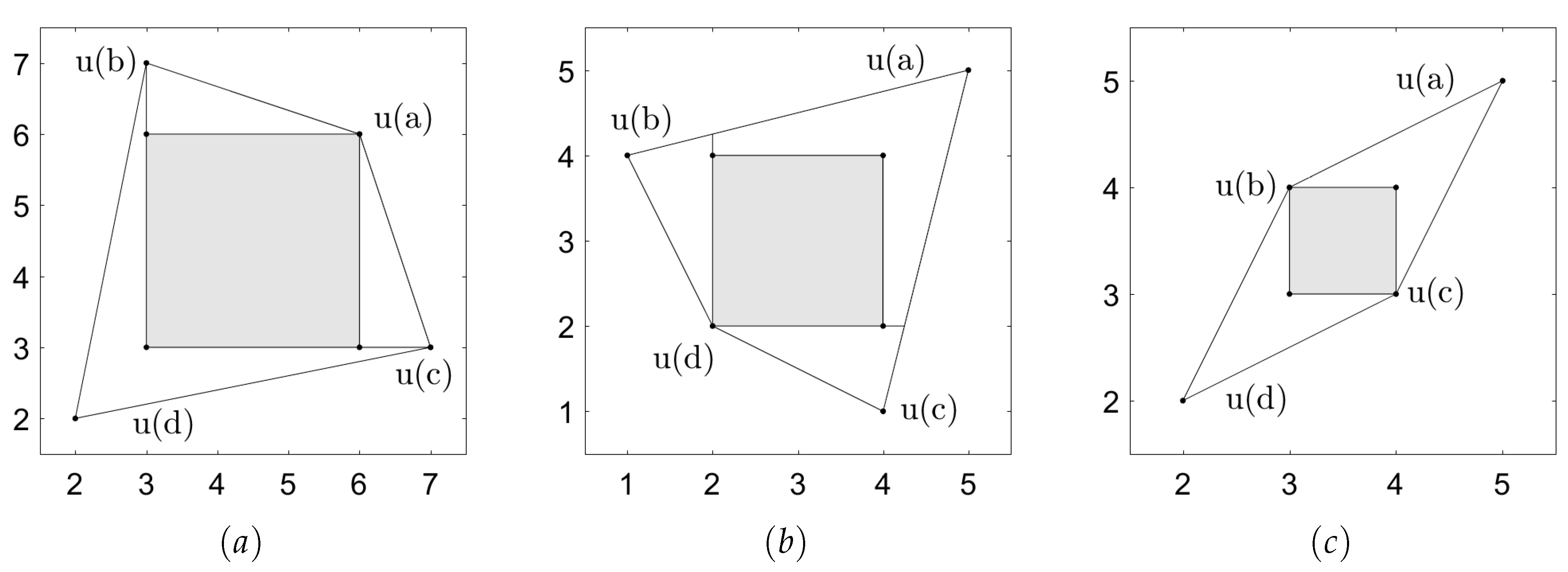
The self-supporting sets and corresponding strategies are useful in the sense that they do not rely on nor require any other equilibrium profiles or payoffs, except for the punishment profiles in the case that a player deviates from his strategy. Thus, if one can find such sets, they are automatically subsets of the equilibrium payoffs. We demonstrate the concept in a prisoner’s dilemma, where a large set of equilibrium payoffs is obtained with surprisingly low discount factor values, and this shows a dramatic difference to the pure-strategy equilibria. See [3,10,11,27,30,31,32,33] for the earlier analysis of prisoner’s dilemma. Moreover, we believe that large, self-supporting sets can be found in many games since they exist, at least, in the following 2 × 2 repeated games: prisoner’s dilemma, stag hunt, chicken and no conflict games (see Figure 1).
It is interesting to compare the set of equilibria in pure, mixed and correlated strategies. It is not clear what the correct model is and it depends on the game situation in hand. Pure strategies may be founded, e.g., in public or governmental decision making where it is unlikely that the players would randomize between the alternatives. This may also be the case with boundedly rational players who may prefer simple strategies rather than playing different mixed strategies on each round the game is played; note, in some models, it is possible to purify mixed-strategy equilibria [34,35]. The mixed strategies can, however, produce higher equilibrium payoffs, as was shown in [24], or decrease the punishment payoffs, which may enlarge the set of equilibria. A higher payoff itself is a reason enough to play mixed strategies, and it is an open problem how to find all mixed-strategy equilibria. In this paper, we show that the interior payoffs in the prisoner’s dilemma can be obtained in mixed strategies with much lower discount factor values compared to the pure strategies. Finally, we note that the correlated strategies are not reasonable in all game situations, since it requires a trusted third party that organizes the public randomization and sends the suitable signals to players so that they can coordinate their actions. We also note that there are many models of correlation in repeated games as the players may receive signals on every round the game is played or only before the first round, and the players may correlate on both pure or mixed strategies.
This paper is structured as follows. Section 2 introduces stage games and the basics of 2 × 2 games. The repeated games are analyzed in Section 3. Section 4 examines a prisoner’s dilemma game. Section 5 demonstrates the self-supporting sets in a quantity-setting duopoly. Section 6 is the conclusion.

2. The Model

2.1. Stage Games

In a repeated game, a stage game is played repeatedly by the same players. A stage game is characterised by the tuple N , A , u , where
  • N = { 1 , , n } is the finite set of players,
  • A i is the finite set of pure actions for player i N , and A = × i N A i is the set of pure-action profiles. Also, a pure action of player i is called a i A i and a pure-action profile is called a A .
  • u R n is the payoff vector.
The play in a stage game: each player i N is allowed to randomize over his pure actions a i A i , yielding a mixed action q i Q i , where Q i is the set of probability distributions over A i , and Q = × i N Q i . So, it holds that q i ( a i ) 0 for each a i A i and a i A i q i ( a i ) = 1 . A pure action is a mixed action as well. A mixed-action profile is denoted by q = ( q 1 , , q n ) Q . The carrier (or support) of a mixed action is the set of pure actions that is played with a strictly positive probability: C a r ( q i ) = { a i A i | q i ( a i ) > 0 } . We also define C a r ( q ) = × i N C a r ( q i ) and for each a C a r ( q ) , we let π q ( a ) be the probability that the action profile a is realized if the mixed-action profile q is played: π q ( a ) = j N q j ( a j ) . The payoffs in a stage game are given by the function u : Q R n . If the players use a mixed-action profile q Q , then player i receives an expected payoff of3
u i ( q ) = a A u i ( a ) π q ( a ) .
Player i’s opponents’ action profile is denoted by q i Q i = × j N , j i Q j . An action profile q is a Nash equilibrium in the stage game if no player has a profitable deviation, i.e.,
u i ( q ) u i ( q i , q i ) for   all i N , and q i Q i .

2.2. Equilibria in 2 × 2 Stage Games

In this subsection, we examine what the sets of equilibrium payoffs can be in 2 × 2 stage games. These games have many classifications [36]. For example, Borm [37] shows that there are 15 classes of games (denoted by c1–c15) based on the players’ best responses. Here, we are interested in three types of games: (i) those that have a two-dimensional set of equilibria (typically Borm’s class c1), (ii) one-dimensional set of equilibria (i.e., one or more line segments; classes c2–c4,c7,c10–c13), and (iii) zero-dimensional set of equilibria (i.e., only one or more points, namely, c5,c6,c9 and c14). We are mostly interested in the first two types of games, since they generate a larger set of payoffs. The following examples demonstrate each type of game.
Games 08 00047 i001
Game 1 has a two-dimensional set of equilibrium payoffs, namely the convex hull of ( 1 , 1 ) , ( 1 , 3 ) , ( 3 , 1 ) and ( 3 , 3 ) . Since both players are always indifferent, any mixed-action pair is an equilibrium. In Game 2, the top action is a strictly dominated action for player 1, and player 2 is indifferent between his actions when player 1 plays the bottom action. Thus, player 2 can play any mixed action when player 1 chooses the bottom action, leading to a one-dimensional set of equilibrium payoffs, namely the line segment 1 , 11 / 3 × 1 . Game 3 is a battle-of-the-sexes game with three equilibria, two in pure actions and one in mixed actions. These generate three payoff points, where the mixed equilibrium gives the lowest payoff of ( 2 / 3 , 2 / 3 ) .

3. Repeated Games

In a repeated game, a stage game is repeated infinitely often and we make the usual assumption that the players only observe the realized pure actions and not the accompanying mixed actions. This so-called public past play is denoted by the set of histories H k = A k = k A for stage k 0 , where H 0 = A 0 = { } and corresponds to the beginning of the game. So, a history contains all the pure-action profiles that have been realized at the previous stages. The set of all histories is H = k = 0 H k . In a repeated game, a public strategy σ i of player i N is a mapping that assigns a probability distribution over player i’s actions for each possible history σ i : H Q i . The set of player i’s strategies is i . The players’ strategies form the strategy profile σ = ( σ 1 , , σ n ) , a strategy profile of all players except player i is denoted by σ i and the set of strategy profiles is given by = × i N i .
Player i discounts the future payoffs with a discount factor δ i ( 0 , 1 ) . The average discounted payoff of a strategy profile σ for player i is
U i ( σ ) = ( 1 δ i ) k = 0 δ i k u i k ( σ ) ,
where u i k ( σ ) is the payoff of player i at stage k induced by the strategy profile σ . A profile σ is a Nash equilibrium if no player has a profitable deviation, i.e.,
U i ( σ ) U i ( σ i , σ i ) for   all i N , and σ i i ,
and it is a subgame-perfect equilibrium (SPE) if it induces a Nash equilibrium in every subgame, i.e.,
U i ( σ | h ) U i ( σ i , σ i | h ) for   all i N , h H , and σ i i ,
where σ | h is the restriction of the strategy profile after history h H .

3.1. Characterization of Equilibria in Repeated Games

The theory of subgame-perfect equilibria in infinitely repeated discounted games with pure strategies has been developed by [1,2,38] (see also [4,10]). The more general model with mixed strategies is analyzed, e.g., in Section 7 in [3].
Let V be the set of subgame-perfect equilibrium payoffs of a repeated game. For any compact set W R n , the punishment payoff of player i in the set W is denoted by
p i ( W ) = min { w i , w W } .
The punishment payoff of player i in the repeated game is the smallest equilibrium payoff, i.e., p i ( V ) . Let us consider an augmented game where the payoff of each action profile a A is given by
u ˜ δ ( a ) ( I T ) u ( a ) + T x ( a ) ,
where T is a diagonal matrix with δ 1 , , δ n on the diagonal. Note that the continuation payoffs x ( a ) are included in the stage-game payoffs. Let M ( x ) , x R | A | × n , be the set of all equilibrium payoffs in this augmented game. Now, we are ready to state the characterization for the subgame-perfect equilibrium payoffs (see Section 7.3 in [3] for the proof).
Theorem 1.
The set V is the largest bounded fixed point of the mapping B:
W = B ( W ) ,
where
B ( W ) = x ( a ) W M ( x ) ,
and the stage game’s payoffs are given by ( I T ) u ( a ) + T x ( a ) , a A .
In contrast to the pure-strategy equilibria, the payoff set V is always non-empty, since every stage game has at least one Nash equilibrium. Note that V is a compact set.
The complexity of computing all mixed-strategy equilibria is much higher compared to the pure-strategy equilibria. Each iteration of B goes through all permutations of all the possible continuations payoffs after each action profile over all action profiles in A.
We denote the payoff set and the mapping B with a discount factor δ by V ( δ ) and B δ . A set W is called self-generating if W B δ ( W ) . The following result follows directly from Theorem 1 (see also Section 7.3 in [3] for generalizations of these results).
Proposition 1.
If a bounded set W is self-generating then B δ ( W ) V ( δ ) .
The following result shows that the payoff set is monotone in the discount factor as long as it is convex. For the next two results, we assume that the players have a common discount factor, which is denoted by scalar δ = δ 1 = = δ n .
Theorem 2.
If V ( δ ) is convex, then V ( δ ) V ( δ ) for scalar δ δ .
It is also possible to show that convex self-generating sets are monotone. The proof is similar to Theorem 2.
Proposition 2.
If a self-generating set W V ( δ ) is convex, then W V ( δ ) for scalar δ δ .

3.2. Self-Supporting Sets and Monotonicity

One problem in finding subgame-perfect equilibria in repeated games is the task of finding the strategy profiles that yield exactly the continuation payoffs such that the players are indifferent between at least two of their pure actions. It turns out that in many games it is possible to find such strategy profiles by selecting the continuation payoffs in such a way that the resulting augmented game corresponds to Game 1 (so with a two-dimensional set of equilibrium payoffs). This means that the play in the repeated game on that round is strategically similar to the play in the one-shot game of Game 1. In the next section, we will show how this construction takes place. It makes use of so-called self-supporting sets that are defined below.
Recall that, for x R | A | × n , the set M ( x ) consists of all equilibrium payoffs in the augmented game where for each a A the continuation payoffs x ( a ) are included in the stage-game payoffs.
Definition 1.
The set S is a self-supporting set if S M ( x ) for some x R | A | × n and if for each payoff s S , (one of) the corresponding equilibrium profile(s) q ( s ) , has the following properties:
1.
a C a r ( q ( s ) ) x ( a ) S , and
2.
if player i plays an action a ˜ i outside C a r ( q i ( s ) ) (an observable deviation), while a i C a r ( q i ( s ) ) , then x i ( a ˜ i , a i ) is player i’s punishment payoff p i ( V ) .
3.
if at least two players make an observable deviation, then the continuation payoff is a predetermined equilibrium payoff.
Furthermore, we say that S is a strongly self-supporting set if it does not rely on the punishment payoffs or if the punishment payoffs are included in the set, i.e., x ( a ) S for all a A . Note that each Nash equilibrium payoff of the stage game by itself forms a strongly self-supporting set. Thus, the self-supporting sets exist in all repeated games but they may not be large or high dimensional.
The difference to the self-generating sets is that the continuation payoffs x ( a ) on the equilibrium path are generated by a single augmented game (the set M ( x ) ) for the self-supporting sets. It also means that the players face the same augmented game on each round, unless there is an observable deviation. Thus, the strategies are simple but not stationary since the players may use different mixed actions after each realized pure-action profile. The strategies on the equilibrium path can be presented with a finite number of states, but they are not of one-period memory [29] (i.e., it is not enough to have the pure-action profiles as states) since some pure-action profile may trigger a punishment in some state but may be acceptable in another state. It should also be noted that the continuation payoffs need not be extreme payoffs, as is the case with correlated strategies and the bang-bang result [3]. The following example [24] shows that self-generating sets are more complicated as they involve multiple stage games with different continuation payoffs.
Example 1.
We examine Prisoner’s Dilemma in Figure 2(a) with δ = 0.25 , and show that the set consisting of ( 1 , 1 ) and two line segments 3.5 × 1.75 , 3.5 and 1.75 , 3.5 × 3.5 is a self-generating set but not self-supporting.
The line segment 3.5 × 1.75 , 3.5 can be generated with Game L1 in Figure 2(b) using continuation payoffs ( 3.5 , 3.5 ) , ( 1 , 1 ) , ( 2 , 3.5 ) and ( 1 , 1 ) . Game L1 can be found by continuing action profile a by path a (a corresponds to ( 3.5 , 3.5 ) , b to ( 0 , 4 ) , c to ( 4 , 0 ) and d to ( 1 , 1 ) ), b and d by path d , and c by a suitable mixed strategy from Game L2 (row player chooses top and column player uses mixed strategy ( 3 / 7 , 4 / 7 ) ). For example, ( 1 δ ) ( 4 , 0 ) + δ ( 2 , 3.5 ) = ( 3.5 , 0.875 ) . All the continuation payoffs belong to the self-generating set itself. The Nash equilibria of Game L1 are the line 3.5 × 1.75 , 3.5 and the point ( 1 , 1 ) . Note that the payoff ( 2 , 3.5 ) is the only one that is outside this set. Game L2 in Figure 2(c) can be found similarly and note that ( 2 , 3.5 ) is an equilibrium payoff in game L2. Thus, these two lines support each other and they are (together with ( 1 , 1 ) ) a self-generating set. This set is not self-supporting as it requires two stage games and two sets of continuation payoffs, and thus this construction is more difficult to find.
The following result shows that certain self-supporting sets are robust in the discount factor if the punishment strategies do not get weaker. This means that the payoffs generated by the self-supporting sets only fill the payoff set more when the players become more patient.
Theorem 3.
Let δ [ 0 , 1 ) and let T be the n × n diagonal matrix with scalar δ on the diagonal. Let S be a self-supporting set for δ and suppose that the following conditions hold:
(i) S is a convex set,
(ii) For all s S with corresponding action profile q ( s ) we have:
u ˜ δ ( a ) = ( I T ) u ( a ) + T x ( a ) S for all a C a r ( q ( s ) ) , and
(iii) p i ( V ( δ ) ) is not increasing in δ for all i N .
Also, let δ δ and let T be the corresponding diagonal matrix. Then there exists a self-supporting set S for δ such that S S .
Proof. 
Let S be a self-supporting set for δ , s S and q ( s ) be an equilibrium profile satisfying the three mentioned properties. We show that the same augmented game payoffs can be obtained for discount factor δ δ , and this does not introduce any profitable unilateral deviations to the players.
First, we show that there exists a continuation payoff x ( a ) S for all a C a r ( q ) such that u ˜ δ ( a ) = u ˜ δ ( a ) , or
( I T ) u ( a ) + T x ( a ) = ( I T ) u ( a ) + T x ( a ) .
From this condition, we get
T x ( a ) = T x ( a ) + T T u ( a )
and thus x ( a ) is between x ( a ) and u ( a ) . Substituting u ( a ) into this equation yields:
( I T ) T x ( a ) = ( T T ) u ˜ ( a ) + ( I T ) T x ( a ) .
This means that x ( a ) is a convex combination of u ˜ ( a ) and x ( a ) . However, since S is convex and u ˜ ( a ) S and x ( a ) S , this implies that x ( a ) S . Moreover, the continuation payoffs are SPE payoffs with δ ; they are generated by the set itself.
It remains to show that there are no profitable deviations that are observable. The incentive compatibility conditions hold for δ :
( 1 δ i ) u ( q ) + δ i w i ( 1 δ i ) d i ( q ) + δ i p i ( V ( δ ) ) ,
for all i N . We show that the same profile q and the continuation payoffs w satisfy these conditions for δ . Let δ i = δ i + ϵ i , where ϵ i 0 . We have:
( 1 δ i ) u i ( q ) + δ i w i = ( 1 δ i ) u i ( q ) + δ i w i ϵ ( u i ( q ) w i ) ( 1 δ i ) d i ( q ) + δ i p i ( V ( δ ) ) ϵ ( u i ( q ) w i ) = ( 1 δ i ) d i ( q ) ϵ u i ( q ) + δ i p i ( V ( δ ) ) + ϵ w i ( 1 δ i ) d i ( q ) ϵ d i ( q ) + δ i p i ( V ( δ ) ) + ϵ p i ( V ( δ ) ) ( 1 δ i ) d i ( q ) + δ i p i ( V ( δ ) )
Here, we used (7) in the first inequality. In the second inequality, we used that d i ( q ) u ( q ) (otherwise there would be no reason to deviate) and that w i p i ( V ( δ ) ) (which follows from x ( a ) p i ( V ( δ ) ) for all a C a r ( q ) by subgame-perfection). Finally, the last inequality follows from p i ( V ( δ ) ) p i ( V ( δ ) ) . Hence, the incentive compatibility constraints are monotone in the discount factor as long as the punishment payoffs do not increase, as observed with pure strategies in Lemma 1 in [10]. ☐
In general, the set of equilibrium payoffs needs not be monotone in the discount factor [25,32,39]. However, if the set of continuation payoffs is convex, e.g., if correlated strategies are available, then the payoff set is monotone in the discount factor [2]. Moreover, if the punishment payoffs are included in the set S, i.e., the set is strongly self-supporting, then the self-supporting set is monotone if it is convex.
Proposition 3.
If S is a convex strongly self-supporting set for scalar δ, then there is a convex strongly self-supporting set S for δ δ such that S S .
We note that Theorem 3 and Proposition 3 could be extended to vector-valued δ if S is additionally assumed to be a hyper-rectangle. This means that the discount factors can be unequal and δ δ means that δ i δ i for all i = 1 , , n . In two-player games, the convex self-supporting sets are always rectangles, which implies that the above results hold for vector-valued δ in these games. The following result gives a sufficient condition for the existence of rectangular self-supporting sets in two-player games.
Proposition 4.
If in a bimatrix game ( A , B ) player 1 has two actions i 1 and i 2 such that b ̲ : = max j b i 1 j < min j b i 2 j = : b ¯ and, similarly, player 2 has two actions j 1 and j 2 such that a ̲ : = max i a i j 1 < min i a i j 2 = : b ¯ , then there exists δ < 1 such that for all δ δ there exists a rectangular self-supporting set a ̲ , a ¯ × b ̲ , b ¯ , where a ̲ = max ( a ̲ , p 1 ( V ( δ ) ) ) and b ̲ = max ( b ̲ , p 2 ( V ( δ ) ) ) .
Proof. 
We can create the following 2 × 2 augmented subgame using actions i 1 , i 2 , j 1 and j 2 .
Games 08 00047 i002
The Nash equilibria of the subgame is the rectangle a ̲ , a ¯ × b ̲ , b ¯ . The continuation payoffs for the actions on the j 2 column (or i 2 row) are all lower than a ¯ ( b ¯ ) since the payoffs on the column (row) are all higher than a ¯ ( b ¯ ). Similarly, the continuation payoffs for the actions on the j 1 column (or i 1 row) are all higher than a ̲ ( b ̲ ’) since the payoffs are all lower than a ̲ ( b ̲ ). Thus, the continuation payoffs belong to the set itself when the discount factor is high enough. Moreover, the players do not have any incentive to deviate outside these two actions when the discount factor is high enough and the deviations are followed by the punishment payoffs that are smaller than or equal to a ̲ or b ̲ . ☐

4. Strategies in the Repeated Prisoner’s Dilemma

In this section, we want to demonstrate the use of self-supporting sets in proving results in repeated games. The results are well-known (see, for example, [27,30,31]). Recall that in symmetric prisoner’s dilemmas all players have the same discount factor denoted by scalar δ .
Games 08 00047 i003
Theorem 4
([30]). In game PD above, the set of subgame-perfect equilibrium payoffs for δ = 1 / 3 is given by the rectangle 1 , 3 × 1 , 3 and the two line segments 3 , 11 / 3 × 1 and 1 × 3 , 11 / 3 .
Proof. 
We first show that the rectangle is a strongly self-supporting set and thus part of the payoff set. Then we show how to get the lines as SPE payoffs and that there are no other SPE payoffs. These results have been developed in [30]4, but here we want to demonstrate the new methodology with an example.
We can create an augmented game from game PD that corresponds to Game 1 by choosing the expected continuation payoffs in the following way: let us denote the action pairs by a, b, c and d, where a corresponds to the payoff ( 3 , 3 ) , b to ( 0 , 4 ) , c to ( 4 , 0 ) and d to ( 1 , 1 ) . If the continuation payoffs are x ( a ) = ( 3 , 3 ) , x ( b ) = ( 3 , 1 ) , x ( c ) = ( 1 , 3 ) , and x ( d ) = ( 1 , 1 ) , then the payoffs in the augmented game are the same as the payoffs in Game 1. For example, after action profile b the payoff is u ˜ ( b ) = ( 1 δ ) ( 0 , 4 ) + δ ( 3 , 1 ) = ( 0 , 8 / 3 ) + ( 1 , 1 / 3 ) = ( 1 , 3 ) . Thus, if the action profile b is realized, then the players continue by playing a strategy pair that gives them a continuation payoff of ( 3 , 1 ) . Now, we show what these ’continuation strategy pairs’ look like for each action profile5.
The action profiles a and d are straightforward. The continuation payoff ( 3 , 3 ) can be obtained by playing action pair a infinitely. We denote this play by a , which is also called a path. So, if an action pair a is realized then the continuation strategy pair is a , and any deviation by any player will be detected and is punished (or followed) by the path d . Similarly, if d is realized, then the continuation payoff ( 1 , 1 ) will be obtained by playing the path d . Finally, the continuation payoff ( 3 , 1 ) (or ( 1 , 3 ) ) can be obtained by playing the action pair c (or b) in Game 1. Thus, in the repeated game, the play will alternate deterministically between b and c if one of these action pairs is realized in the augmented game at stage 1. We denote this play by ( c b ) after b and ( b c ) after c. Note that the equilibrium payoffs in Game 1 form the rectangle [ 1 , 3 ] × [ 1 , 3 ] and all the required continuation payoffs are contained in this set as well. So, [ 1 , 3 ] × [ 1 , 3 ] is actually a strongly self-supporting set, since it even contains the punishment payoffs.
Now, we show that the payoffs on the line segment 3 , 11 / 3 × 1 can be obtained by subgame-perfect equilibria (a similar argument holds for the line segment 1 × 3 , 11 / 3 ). We will show that we can create an augmented game at stage 1 of game PD that corresponds to Game 2. To do this, we let the action pairs a, b and d be followed by the path d , and c be followed by the path a . Then, e.g., u ˜ ( c ) = ( 1 δ ) ( 4 , 0 ) + δ ( 3 , 3 ) = ( 11 / 3 , 1 ) . However, the ( 3 , 3 ) continuation payoff is not in the set 3 , 11 / 3 × 1 . This means that the line segment is not a self-supporting set: it requires a continuation payoff that is outside the set.
It remains to show that there are no other subgame-perfect equilibrium payoffs. Assume on the contrary that there is a subgame-perfect equilibrium payoff ( 3 + w 1 , 1 + w 2 ) , where w 1 , w 2 > 0 . It is easy to check that this payoff can only be obtained by playing first the action profile c. To generate the payoff, the continuation payoff ( x 1 , x 2 ) must satisfy u ˜ ( c ) = ( 1 δ ) ( 4 , 0 ) + δ ( x 1 , x 2 ) = ( 3 + w 1 , 1 + w 2 ) . From this, we get x 1 = 1 + 3 w 1 and x 2 = 3 + 3 w 2 . This continuation payoff itself can only be obtained by playing action profile b first. The required continuation payoff after b turns out to be ( 3 + 9 w 1 , 1 + 9 w 2 ) > ( 3 + w 1 , 1 + w 2 ) . We can conclude that this process requires higher and higher continuation payoffs, which will eventually be outside the convex hull of the stage-game payoffs, and thus they cannot be generated by the repeated game. ☐
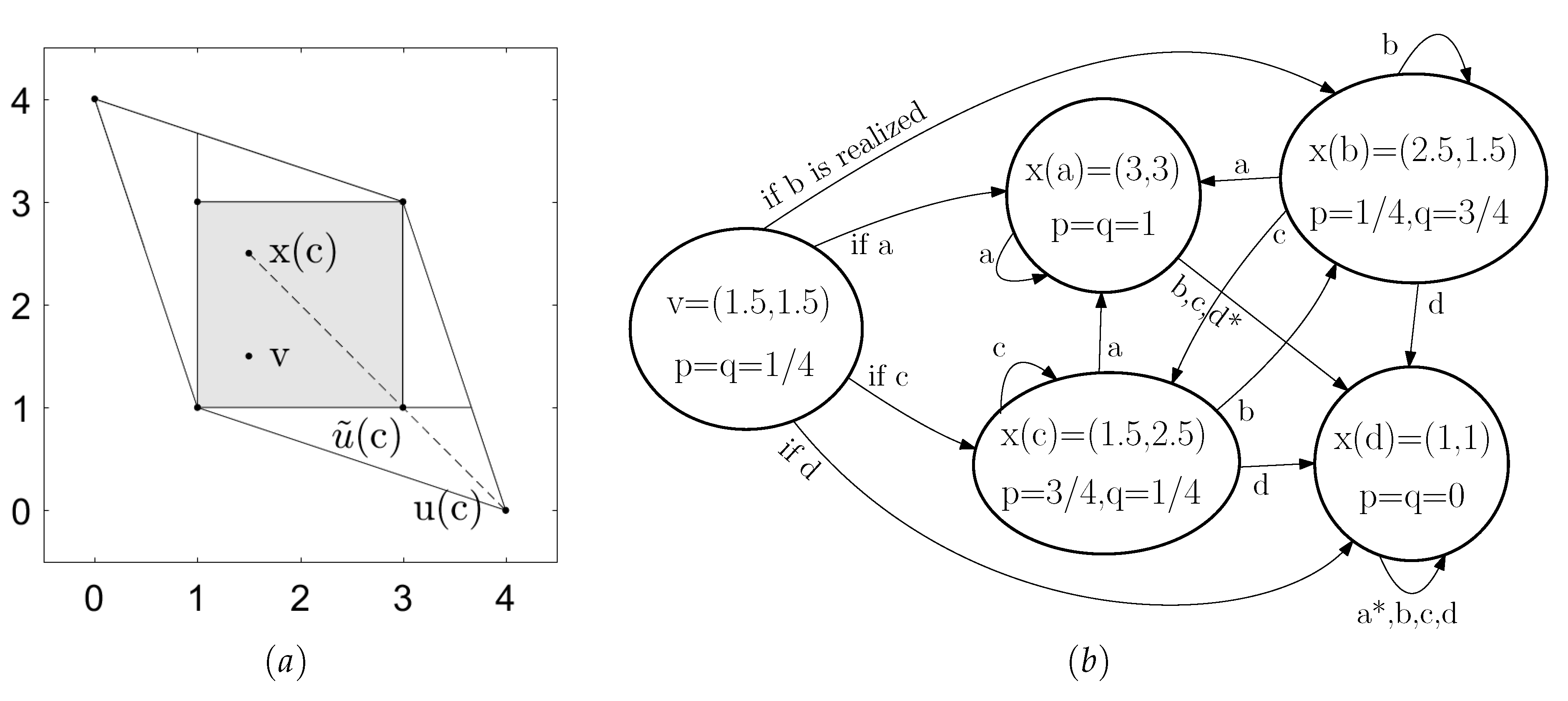
Figure 3a illustrates a strongly self-supporting set in game PD with δ = 2 / 5 , and b the corresponding strategies with a finite number of states. Figure 3a shows that the continuation payoff x ( c ) belongs to the shaded self-supporting set, and v = ( 1.5 , 1.5 ) is an arbitrary point in the set. It holds that u ˜ ( c ) = ( 1 δ ) u ( c ) + δ x ( c ) , which geometrically means that u ˜ ( c ) is δ = 0.4 fraction on the line from u ( c ) to x ( c ) . When δ = 1 / 3 , x ( c ) moves to the corner point ( 1 , 3 ) , which is the smallest δ value when the self-supporting set exists. In Figure 3b, we can see the equilibrium strategy pair that produces payoff v. Each circle corresponds to a state with the expected payoffs and the action pair that is played in that state. The states that the arrows point to correspond to the action pairs that should be played next. The probabilities of top and left actions are given by p and q for the row and column players, respectively. The star denotes that the corresponding transition could be to any equilibrium strategy, since it corresponds to the case where both players deviate from the equilibrium strategy simultaneously. Note that the continuation play involves mixed strategies in general, unless the continuation payoff happens to be one of the pure payoffs.
Theorem 5.
In game PD, for δ 1 / 3 , the rectangle 1 , 3 × 1 , 3 is a subset of the set of subgame-perfect equilibrium payoffs.
Proof. 
Using the fact that 1 , 3 × 1 , 3 is a convex strongly self-supporting set, this follows directly from combining Proposition 3 or Theorem 3 with the proof of Theorem 4. ☐
Games 08 00047 i004
Theorem 6.
In game PD2, a symmetric prisoner’s dilemma, the rectangle d , a × d , a is a subset of the set of subgame-perfect equilibrium payoffs for
δ max c a c d , d b a b .
Proof. 
We want to find the smallest discount factor for which the set d , a × d , a is strongly self-supporting. This means that the continuation payoff x ( c ) after action pair c must satisfy u ˜ ( c ) = ( 1 δ ) ( c , b ) + δ ( x 1 ( c ) , x 2 ( c ) ) = ( a , d ) . This gives
( x 1 ( c ) , x 2 ( c ) ) = a ( 1 δ ) c δ , d ( 1 δ ) b δ ,
where, in order to make the set self-supporting, we require that x 1 ( c ) d and x 2 ( c ) a , leading to δ max ( c a ) / ( c d ) , ( d b ) / ( a b ) . ☐

5. Example of a Duopoly Game

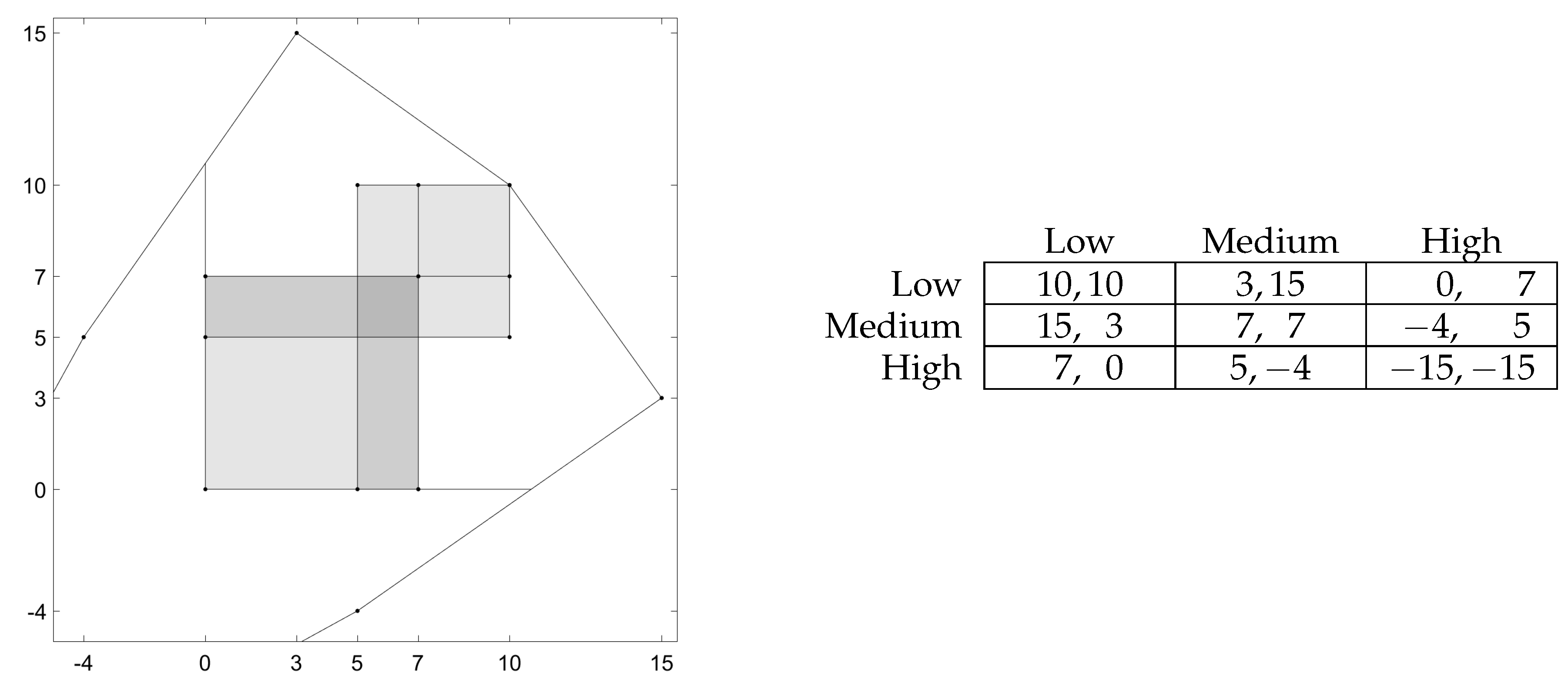
Let us examine the duopoly model of Abreu [38], where two firms decide their production quantities. The firms have three output levels: low (L), medium (M) and high (H) (see Figure 4). The stage game’s Nash equilibrium is (M,M), which gives the players the payoff ( 7 , 7 ) . The players may obtain many other equilibrium payoffs in the repeated game, including the payoff ( 10 , 10 ) which is obtained by playing (L,L) repeatedly. This outcome is supported by the punishment6 of playing H, which makes the other player obtain, at most, a payoff of 0. In this paper, we show that large sets of payoffs can be obtained using self-supporting sets.
Figure 4 shows four self-supporting sets that exist when the players are patient enough: the squares 0 , 7 × 0 , 7 and 7 , 10 × 7 , 10 , and the rectangles 0 , 10 × 5 , 7 and 5 , 7 × 0 , 10 . These are equilibrium payoffs and they cover almost half of the feasible and individually rational payoffs. The equilibrium payoffs depend on the discount factors and it is difficult to find all of them, however, these self-supporting sets capture majority of them.
The self-supporting sets in games with more actions can be found by splitting the game into smaller 2 × 2 games. Randomizing between more than two actions does not bring any new payoffs for the self-supporting sets, and it is more difficult to find the suitable continuation payoffs in the set such that the players are indifferent between all the actions. In this game, the square 0 , 7 × 0 , 7 can be found in the No Conflict game in Figure 5a. The square 7 , 10 × 7 , 10 can be found in Prisoner’s Dilemma game in Figure 5b. The rectangle 0 , 10 × 5 , 7 can be found in Game D1 in Figure 5c, and the other rectangle symmetrically by switching the role of the players.
Note that it is easy to find the self-supporting sets in 2 × 2 games by Proposition 4. If the minimum payoff against one action is higher than the maximum payoff against the other action and this holds for both players, then the self-supporting set contains all the payoffs between the maximum and the minimum payoffs. In Game D1, the minimum payoff of player 1 against L is 10 and the maximum against H is 0, and the minimum payoff of player 2 against L is 7 and the maximum payoff against M is 5. Thus, the self-supporting set is 0 , 10 × 5 , 7 . It is easy to check geometrically that the continuation payoffs belong to the set when the discount factors are high enough.

6. Conclusions

In this paper, we construct subgame-perfect mixed-strategy profiles in repeated games. Basically, the players consider on each round an augmented game that takes into account the continuation payoffs that are defined by the players’ follow-up strategies. The continuation play and payoffs can be different after each realized pure-action profile but all the continuation payoffs need to be equilibrium payoffs themselves. Moreover, the equilibrium payoffs can be found by computing the Nash equilibria in all these augmented games.
How to compute the mixed-strategy equilibria efficiently is still an open problem. It is more difficult to compute all the mixed-strategy equilibria compared to the pure (or correlated) strategies. However, we have found that the concept of self-supporting sets may facilitate our task considerably, since they may give us large and high-dimensional sets of equilibrium payoffs with relatively simple accompanying strategy profiles. It is left to future research to determine how common large self-supporting sets are in multiplayer games and under which conditions they do exist. Although, it may be very hard to find all the equilibrium payoffs and corresponding strategy profiles, it may be possible to compute some payoffs or good approximations fast. We think that our concept of self-supporting sets may open up ideas for new simple strategies that produce large sets of payoffs in repeated and stochastic games.

Acknowledgments

Kimmo Berg acknowledges funding from Emil Aaltosen Säätiö through Post doc -pooli.

Author Contributions

Kimmo Berg and Gijs Schoenmakers developed the main idea and wrote the paper together. Kimmo Berg developed the numerical examples and illustrations.

Conflicts of Interest

The authors declare no conflict of interest.

References

  1. Abreu, D.; Pearce, D.; Stacchetti, E. Optimal cartel equilibria with imperfect monitoring. J. Econ. Theory 1986, 39, 251–269. [Google Scholar] [CrossRef]
  2. Abreu, D.; Pearce, D.; Stacchetti, E. Toward a theory of discounted repeated games with imperfect monitoring. Econometrica 1990, 58, 1041–1063. [Google Scholar] [CrossRef]
  3. Mailath, G.J.; Samuelson, L. Repeated Games and Reputations: Long-Run Relationships; Oxford University Press: Oxford, UK, 2006. [Google Scholar]
  4. Cronshaw, M.B.; Luenberger, D.G. Strongly symmetric subgame perfect equilibria in infinitely repeated games with perfect monitoring. Games Econ. Behav. 1994, 6, 220–237. [Google Scholar] [CrossRef]
  5. Cronshaw, M.B. Algorithms for finding repeated game equilibria. Comput. Econ. 1997, 10, 139–168. [Google Scholar] [CrossRef]
  6. Judd, K.; Yeltekin, Ş.; Conklin, J. Computing supergame equilibria. Econometrica 2003, 71, 1239–1254. [Google Scholar] [CrossRef]
  7. Burkov, A.; Chaib-draa, B. An approximate subgame-perfect equilibrium computation technique for repeated games. In Proceedings of the Twenty-Fourth AAAI Conference on Artificial Intelligence, Atlanta, GA, USA, 11–15 July 2010; pp. 729–736. [Google Scholar]
  8. Salcedo, B.; Sultanum, B. Computation of Subgame-Perfect Equilibria of Repeated Games with Perfect Monitoring and Public Randomization; Working Paper; The Pennsylvania State University: State College, PA, USA, 2012. [Google Scholar]
  9. Abreu, D.; Sannikov, Y. An algorithm for two player repeated games with perfect monitoring. Theor. Econ. 2014, 9, 313–338. [Google Scholar] [CrossRef]
  10. Berg, K.; Kitti, M. Equilibrium Paths in Discounted Supergames; Working Paper; Aalto University: Espoo, Finland, 2012; Available online: http://sal.aalto.fi/publications/pdf-files/mber09b.pdf (accessed on 24 October 2017).
  11. Berg, K.; Kitti, M. Computing equilibria in discounted 2 × 2 supergames. Comput. Econ. 2013, 41, 71–78. [Google Scholar] [CrossRef]
  12. Berg, K.; Kitti, M. Fractal geometry of equilibrium payoffs in discounted supergames. Fractals 2014, 22. [Google Scholar] [CrossRef]
  13. Fudenberg, D.; Maskin, E. The folk theorem in repeated games with discounting and incomplete information. Econometrica 1986, 54, 533–554. [Google Scholar] [CrossRef]
  14. Fudenberg, D.; Maskin, E. On the dispensability of public randomization in discounted repeated games. J. Econ. Theory 1991, 53, 428–438. [Google Scholar] [CrossRef]
  15. Gossner, O. The Folk Theorem for Finitely Repeated Games with Mixed Strategies. Int. J. Game Theory 1995, 24, 95–107. [Google Scholar] [CrossRef]
  16. Busch, L.-A.; Wen, Q. Negotiation games with unobservable mixed disagreement actions. J. Math. Econ. 2001, 35, 563–579. [Google Scholar] [CrossRef]
  17. Fudenberg, D.; Levine, D.; Maskin, E. The folk theorem with imperfect public information. Econometrica 1994, 62, 997–1039. [Google Scholar] [CrossRef]
  18. Sugaya, T. Characterizing the limit set of PPE payoffs with unequal discounting. Theor. Econ. 2015, 10, 691–717. [Google Scholar] [CrossRef]
  19. Chassang, S.; Takahashi, S. Robustness to incomplete information in repeated games. Theor. Econ. 2011, 6, 49–93. [Google Scholar] [CrossRef]
  20. Peski, M. Repeated games with incomplete information and discounting. Theor. Econ. 2014, 9, 651–694. [Google Scholar] [CrossRef]
  21. Dutta, P.K. A Folk theorem for stochastic games. J. Econ. Theory 1995, 66, 1–32. [Google Scholar] [CrossRef]
  22. Hörner, J.; Sugaya, T.; Takahashi, S.; Vieille, N. Recursive methods in discounted stochastic games: An algorithm for δ → 1 and a folk theorem. Econometrica 2011, 79, 1277–1318. [Google Scholar]
  23. Berg, K. Elementary subpaths in discounted stochastic games. Dyn. Games Appl. 2016, 6, 304–323. [Google Scholar] [CrossRef]
  24. Berg, K. Set-Valued Games and Mixed-Strategy Equilibria in Discounted Supergames; Working Paper; Aalto University: Espoo, Finland, 2017. [Google Scholar]
  25. Berg, K. Extremal pure strategies and monotonicity in repeated games. Comput. Econ. 2017, 49, 387–404. [Google Scholar] [CrossRef]
  26. Berg, K.; Kärki, M. An Algorithm for Computing the Minimum Pure-Strategy Payoffs in Repeated Games; Working Paper; Aalto University: Espoo, Finland, 2016; Available online: http://sal.aalto.fi/publications/pdf-files/mber14c.pdf (accessed on 24 October 2017).
  27. Ely, J.C.; Välimäki, J. A Robust Folk Theorem for the Prisoner’s Dilemma. J. Econ. Theory 2002, 102, 84–105. [Google Scholar] [CrossRef]
  28. Ely, J.C.; Hörner, H.; Olszewski, W. Belief-free equilibria in repeated games. Econometrica 2005, 73, 377–415. [Google Scholar] [CrossRef]
  29. Doraszelski, U.; Escobar, J.F. Restricted feedback in long term relationships. J. Econ. Theory 2012, 147, 142–161. [Google Scholar] [CrossRef]
  30. Sorin, S. On repeated games with complete information. Math. Oper. Res. 1986, 11, 147–160. [Google Scholar] [CrossRef]
  31. Stahl, D.O. The graph of prisoner’s dilemma supergame payoffs as a function of the discount factor. Games Econ. Behav. 1991, 3, 368–384. [Google Scholar] [CrossRef]
  32. Mailath, G.J.; Obara, I.; Sekiguchi, T. The maximum efficient equilibrium payoff in the repeated prisoners’ dilemma. Games Econ. Behav. 2002, 40, 99–122. [Google Scholar] [CrossRef]
  33. Berg, K.; Kärki, M. How Patient the Players Need to Be to Obtain All the Relevant Payoffs in Discounted Supergames? Working Paper; Aalto University: Espoo, Finland, 2014; Available online: http://sal.aalto.fi/publications/pdf-files/mber14b.pdf (accessed on 24 October 2017).
  34. Bhaskar, V.; Mailath, G.J.; Morris, S. Purification in the infinitely-repeated prisoners’ dilemma. Rev. Econ. Dyn. 2008, 11, 515–528. [Google Scholar] [CrossRef]
  35. Bhaskar, V.; Mailath, G.J.; Morris, S. A foundation for Markov equilibria in sequential games with finite social memory. Rev. Econ. Stud. 2013, 80, 925–948. [Google Scholar] [CrossRef]
  36. Robinson, D.; Goforth, D. The Topology of the 2 × 2 Games: A New Periodic Table; Routledge: Abingdon, UK, 2005. [Google Scholar]
  37. Borm, P. A classification of 2 × 2 bimatrix games. Cah. Cent. d’Etudes Rech. Oper. 1987, 29, 69–84. [Google Scholar]
  38. Abreu, D. On the theory of infinitely repeated games with discounting. Econometrica 1988, 56, 383–396. [Google Scholar] [CrossRef]
  39. Yamamoto, Y. The use of public randomization in discounted repeated games. Int. J. Game Theory 2010, 39, 431–443. [Google Scholar] [CrossRef]
1.
Figure 1 (and also the example in Section 5) shows that the self-supporting sets may produce a large portion of the area of the feasible and individually rational payoffs in the game and thus even larger portion of the equilibrium payoffs.
2.
Only the strategy on the equilibrium path is guaranteed to have a finite presentation but we are not aware of any result that the punishment strategies have a finite presentation.
3.
Note that u i ( a ) denotes the stage-game payoffs and u i ( q ) the expected payoff of a mixed strategy q.
4.
We thank Tadashi Sekiguchi for pointing this out.
5.
Note that in general the continuation play involves mixed strategies even though pure strategies are enough in this example. Figure 3b shows an example where mixed actions are used after action profiles b and c.
6.
The optimal pure punishment strategies in this game depend on the discount factors [26].
Figure 1. Self-supporting sets in (a) chicken, (b) stag hunt and (c) no conflict games. The players’ payoffs of action profiles a, b, c and d are denoted by u ( a ) to u ( d ) , respectively.
Games 08 00047 g001
Figure 2. Prisoner’s dilemma and the stage games used in constructing a self-generating set.
Games 08 00047 g002
Figure 3. Geometric illustration of (a) a self-supporting set and (b) the strategies in game PD. The star denotes that the corresponding transition could be to any equilibrium strategy.
Games 08 00047 g003
Figure 4. Four self-supporting sets in a duopoly game with three production quantities.
Games 08 00047 g004
Figure 5. Subgames used in constructing the self-supporting sets in the duopoly game.
Games 08 00047 g005