Equilibrium Analysis for Platform Developers in Two-Sided Market with Backward Compatibility


School of Management, Kyung Hee University, Seoul 02447, Korea
Games 2018, 9(4), 76; https://doi.org/10.3390/g9040076
Submission received: 29 June 2018
/
Revised: 7 September 2018
/
Accepted: 28 September 2018
/
Published: 1 October 2018
(This article belongs to the Special Issue Games and Industrial Organization)
Abstract
:We consider a dominant platform provider operating both legacy and new platforms that connects users with suppliers in a two-sided market context. In addition to the typical indirect network effects in the two-sided market, backward compatibility works on the new platform. Thus, users joining the new one can also enjoy the services provided by suppliers using the legacy platform. Users and suppliers are linearly differentiated between two platforms as in the Hotelling model and play a subscription game of choosing one platform at the lower level. The suppliers in the new platform may suffer from congestion, which can be alleviated by platform provider’s investment on the new one. The platform provider also determines price margins for the supplier sides. Our equilibrium (eq.) analysis in the subscription game identifies an interior eq. (coexistence of both platforms in both sides). Though the backward compatibility plays a stabilizing role for the interior eq., its stability is fragile due to the network effects. Rather, some boundary eq.’s, where at least one side tips to the legacy or the new platform, are more likely to be stable. The backward compatibility is a key factor that characterizes the stable boundary eq.’s. The upper stage game is led by the platform provider, which tries to maneuver the system toward one of the stable boundary eq.’s using price margins and investment. The platform provider prefers an all-new boundary eq. when the indirect network effect and the maximum price margin for the new platform are large; thus, it puts a significant investment in the new one. With a small indirect network effect for suppliers, however, the platform provider does not invest in the new platform and choose a separate boundary eq. where two sides split into different platforms. Whether the user side completely tips to the new one (completely separated eq.) or not (partially separated eq.) depends on the backward compatibility. The relative advantage of the all-new eq. over the separate eq.’s in terms of social welfare from both sides depends on the backward compatibility as well as the indirect network effects for the new platform.
1. Introduction
Two-sided market models provide a new perspective to view the platform industries such as credit cards, newspapers, telecommunications, Internet services, and many others (see References [1,2,3] for more examples of the two-sided markets). In a two-sided market, two distinct parties are connected to each other through a platform that constitutes a set of the institutional agreements necessary to realize a transaction between these parties [2,4]. A key characteristic here is the presence of network externalities or network effects between the two groups. Thanks to the network effects, the market power of a dominant platform is expected to be quite stable across generations. Platform providers of operating systems (OS; e.g., Windows, iOS, Android, etc.) and social network services (SNS; e.g., Facebook) present representative examples of this kind of successive dominance.
Persistent dominance over successive generations in a two-sided market, however, requires a special type of network effect that enables the maintenance of compatibility between current and new generations: that is, the backward compatibility. The representative global platforms introduced above suggest an important role of the backward compatibility for sustaining their dominant positions. However, different platform industries show different patterns of platform management (old vs new vs both) in the presence of the backward compatibility. For example, some users of PC OS (e.g., Windows) take their automatic OS version updates in stride and others do not (as of May 2018, 31.3% for Windows 10.x vs 43.8% for Windows 7.x worldwide, source: https://www.netmarketshare.com), while suppliers (third-party software providers) are quite slow in adjusting their applications to the latest version. On the other hand, both users and suppliers (app developers) of iPhone iOS promptly upgrade their programs and toolkits to the new version of the OS. It did not take a long time for the latest iOS version (iOS 11.x) to reach more than 70% after its first release in 2017 spring (as of 27 June 2018, 78.0% for iOS 11.x vs 11.7% for iOS 10.x worldwide, source: https://david-smith.org/iosversionstats).
Though the backward compatibility is crucial for strategic decisions of the platform providers, especially planning to upgrade their platforms, many studies on the two-sided markets have paid little attention to this feature. To our knowledge, there have been few studies presenting a stylized game model for this issue. We explicitly deal with the version management of a dominant platform provider and the role of the backward compatibility together with other typical features in the two-sided markets (e.g., indirect network effects).
The paper is organized as follows. In the next section, we present some prior works relevant to the two-sided market and compatibility issues. Section 3 presents a stylized model incorporating the backward compatibility into a two-sided market framework developed on the basis of Hotelling’s linear differentiation model. The second half of this section analyzes various equilibria and their stabilities. In the next section, we conduct analyses of a dominant platform provider’s decisions on its platform upgrade and present some experimental results to confirm the analyses. Lastly, Section 5 summarizes key findings, discusses implications of this study to platform strategy, and concludes the paper by providing future research directions.
2. Two-Sided Market and Compatibility: Literature Review and Our Approach
Studies on two-sided markets could have been developed around the compatibility issues. When References [5,6] paid attention to the paradigm shift in the software industries and introduced the notion of the indirect network effect, the compatibility in the system markets [7,8,9] was one of the key features to study: for example, product compatibility with rivals and cross-generational (or vertical) compatibility. Early studies on the two-sided markets such as References [10,11] also touched on some issues regarding the compatibility under competition and the backward compatibility. Number-theoretical studies on the two-sided markets, however, focused on a pricing structure designed by a platform and strategic implications or empirical tests of the indirect network effects in practice. Our study aims at incorporating not only typical core features of the two-sided markets—indirect network effect and price structure—but also the backward compatibility into a stylized model.
Our survey starts with theoretical literature on the network effects and the two-sided markets, which includes some early works like [1,2,3,10,11,12,13,14], to name a few. They provide widely applicable models and deal with markets for credit cards, console games, PC software, advertising through web portals and yellow pages, etc. ([4,15]), which provide an excellent overview of the two-sided market studies. The majority of the two-sided market studies focus on the pricing structure together with a subsidization strategy across two sides since it serves as a fundamental driver for maximizing profits of the platforms in the two-sided markets. Not much attention, however, has been paid to the compatibility issues, in particular, the backward compatibility arising at the moment of migration from the current to a new platform. For competing platforms, much attention has been paid to changes in the competitive landscape with switching costs or compatibility. For example, Reference [16] considers the interaction effects of switching costs and network externality in a dynamic game frame. It identifies the conditions of overturning the classical U-shaped relationship between the degree of switching costs and platform’s pricing levels. As a result, lowering switching costs does not guarantee an improvement of the social welfare. Reference [17] deals with the issue of switching costs in the two-sided markets, where the switching costs are endogenously determined. Moreover, by considering content procurement control and sequential entry of the platform, it reveals that the structure and origin of the switching costs are also the key elements of the competition.
Compatibility with a rival’s product or service under network effects as in telephone networks [5,18,19,20,21,22] has drawn particular interests. Here, incompatibility could produce a tipping, where all the new customers join one network [23]. Reference [6] presents a dynamic model where competing firms may have an incentive to implement compatibility in their products to supplement price competition. Along this line, Reference [24] shows that compatibility may be utilized for alleviating research and development (R&D) competition at the stage of new product development. References [25,26] also present strategic aspects of compatibility with complementary products. Reference [27] develops a dynamic model which deals with consumer entrance choice upon the chance of emerging new technology. Reference [28] provides a two-stage game model for compatibility choice decision and suggests the notion of planned obsolescence. This research track could have naturally extended to competing platforms in a two-sided market. However, there have not been many studies addressing the compatibility issue in a two-sided market except the following.
However, the compatibility issue in the two-sided markets has been mostly addressed within the context of platform competition. Reference [29] examines the effect of users’ multi-homing decisions on compatibility between two networks. Reference [30] extends the frameworks of [27,28], and provides a stylized model for compatibility mode choice (“compatibility regime” in their term) to explain how the mode choice depends on some characteristics (e.g., interdependence of installed bases and market growth rate) of the two-sided markets. Reference [31] deals with a monopoly platform in a two-sided market, which has an incentive to maintain incompatibility for foreclosing competition in its complementary market. Reference [32] also extends the scheme of planned obsolescence [28] to the two-sided markets. References [17,33] examine the cases of competing platforms, where incompatibility gives rise to benefits for dominant platform player. Reference [34] studies compatibility mode choice of two competing platforms in a two-sided market. They also show how each phase of the product life cycle affects the compatibility strategy of platforms. References [4,35] focus on the inter-generational nature of information technology (IT) services via the backward compatibility as well as the typical indirect network effect in the two-sided markets. Both provide empirical results for particular platform industries: Reference [35] for hand-held video console games and Reference [4] for wireless carriers’ mobile Internet services. Both also address the mechanism of the double-edged sword nature of the backward compatibility—i.e., a tool for extending the lifespan of existing platforms and a catalyst for migration toward new platforms—and show these effects in their respective industries. Among these studies, however, only References [30,35,36] directly address the backward compatibility in the two-sided market framework.
The primary interest of this study is also the roles of the backward compatibility as well as other typical features of the two-sided markets (i.e., indirect network effects and pricing structure) in platform switch. However, our perspective and approach to the backward compatibility are quite different from those in the prior studies. First of all, the main research objective here is to address the platform selection issue in a more general two-sided market context. Thus, when developing a model, we do not have a particular digital service in mind, while References [4,30,35] are all closely related with the game console industries. Instead, the study background in mind is broader IT service platforms (e.g., OS platforms in mobile and personal computer (PC), SNS platforms, etc.), which do not necessarily depend on durable complementary goods like a game console.1
Our approach is clearly different from those in the empirical studies like References [35,36] since we build a conceptual, stylized model to frame the backward compatibility issue from the two-sided market perspective. In this sense, we pursue a similar track to the one in Reference [30]. For example, we also develop a stage game model including the platform development decision of a dominant platform provider. However, their context and modeling approach is very different from ours. Reference [30] considers the backward compatibility as a decision variable (similar to the role of the converter in Reference [20]) of a monopoly platform provider. Furthermore, their model is constructed on the diffusion scheme employed in Reference [27] for deriving a dynamic implication from the perspective of market growth. By contrast, our main focus is not to determine an optimal level of the backward compatibility, but to identify a platform selection as an equilibrium (hitherto undiscovered or insufficiently dealt with in the two-sided market studies). Thus, we sacrifice the endogeneity of the backward compatibility in our modeling. Instead, we are now free of presuming a set of compatibility regimes (possible configurations of compatibility implementation across two platforms) employed in Reference [30]. Furthermore, our perspective on the dynamics of the platform development suggests a stability analysis so that we can verify whether a candidate equilibrium (i.e., a possible compatibility mode) is sustainable or not.
In our modeling and analysis section, one could also easily find out many different aspects between this study and the previous ones. For example, we do not consider the possibility of technological breakthrough across the successive platforms [28,30]. Instead, we assume that the technological difference between the two platforms is modest. While our model incorporates possible price discrimination between two platforms as in Reference [28,37] (however, neither in the two-sided market framework), it focuses on a margin of price discrimination within which the platform provider could utilize its pricing strategy. We are also interested in the investment decision of the dominant platform provider for alleviating congestion in a new platform, which is a quite common problem in IT service platforms.
Last but not least, the equilibrium analysis here will be somehow new to traditional economics literature. In addition to the traditional interior equilibrium, we pay much attention to the boundary equilibria, each of which represents an extreme compatibility mode. Furthermore, we analyze not only static equilibria but also their stabilities in terms of system dynamics. Accordingly, despite the static nature of the equilibria, we could provide some insights to the dynamics of platform selection with regard to the backward compatibility as well as other key features of the two-sided markets.
3. Baseline Model and Equilibrium Analysis
3.1. Baseline Model: Structure, Players, and Payoffs
We consider a monopoly or a dominant platform provider that operates two platforms A and B. Without loss of generality, we assume that those platforms A and B are based on the current technology and new emerging technology, respectively. Both platforms connect suppliers and users, thereby exerting the indirect network effect in a two-sided market explained in the previous sections. Even when both platforms share the same ownership, two platforms may virtually compete to achieve the market share in each side. This will happen when a new version of the platform was developed in a different department of the same platform provider. Or, a platform provider (as part of its business strategy) may let different versions of the platform be selected through a competition in the marketplace. Release of new version for OS will be an example of this case.
In this study, we consider the case where the new platform (B) provides all the services that the current platform (A) does. For example, platform B represents a recent version of mobile OS that runs most apps developed for the previous OS version. Another example is a newly deployed fast line Internet connection that guarantees high-resolution video streaming (e.g., UHD Netflix service) as well as traditional Internet services like email and web surfing. Thus, platform B is “backward compatible” in the sense that it may accommodate all the services designed for platform A.
The backward compatibility may be related to the vertical as well as the horizontal differentiation. This study, however, focuses on the latter and postulates the relevant contexts, for example, technically savvy users or early adopters (e.g., children of adolescence) who prefer a new platform version to the old one versus technically insensitive users or followers (e.g., middle-aged parents). In this context, Apple and Samsung are releasing a new version of their smartphones every year while retaining the old versions for a while. Google’s Android version management and telcos’ network infrastructure transition (e.g., 3G to 4G/LTE) can also be understood in the same vein.
Under the context described above, we develop a stylized model as follows. Our demand model assumes that both users and suppliers are horizontally differentiated based on their preferences for two distinct platform versions a la Hotelling [38]. That is, a user (a supplier) is situated on an interval , and this location reveals his/her preferences for both platforms. Here, we employ () for the user index (the supplier index) representing his/her preference to the platforms. Without loss of generality, the left end point of the interval () is supposed to represent the user (the supplier) who most prefers A to B, while the right end point () represents the index of the player who most prefers B to A: that is, for the extreme platform-A-lover and for the extreme platform-B-lover. Following the convention of the Hotelling model, users are uniformly populated over the line segment. This normalization of the horizontal differentiation implies that our model focuses on the market share in each side. The same configuration is applied to the supplier side (refer to Figure 1).
Now, we incorporate the traditional features of the two-sided markets: indirect network effects. First, represents the indirect network effect in the user side for platform k (k = either A or B). That is, represents how users in platform k benefit from the supplier side on the same platform. Similarly, let denote the indirect network effect in the supplier side for platform k (k = A, B). We set the network effects in platform A— and —at , and focus on the relative effects of network effects between the platforms. In this way, we can save the subscripts, and let and respectively represent the corresponding indirect network effects for the users and the supplier in platform B.
We also introduce the cross-platform network effect , which, by definition, measures users’ benefits from the backward compatibility in the new platform (B). Users subscribing to platform B enjoy not only the services that suppliers in platform B provide but also the ones provided by suppliers in platform A. For example, users of a fast Internet connection (e.g., Google fiber) are able to access premium services (e.g., UHD video streaming) as well as traditional services that are insensitive to delay (e.g., email). Those who update their iPhone OS, say to iOS 11.x, are also able to use most apps developed for iOS 10.x. Note that, however, this effect is “asymmetric”. works only for platform B thanks to the backward compatibility, and it directly benefits users, not suppliers.2 Furthermore, means that there is no benefit from the directional interactions between the users in the new platform and the suppliers in the legacy platform: that is, no backward compatibility.
The backward compatibility of platform B may come at the cost of congestion, or negative network externality in the new platform, especially when this platform is in the early phase of the life cycle. We consider this kind of congestion effect on the suppliers, and employ to denote the degree of congestion (or the negative network externality) in the supplier side of platform B. However, we also consider a countermeasure that the platform provider carries out in order to alleviate this negative externality. As the platform provider makes investment in the new platform, it enhances its capability to accommodate more suppliers and provides better quality of service through this platform. Thus, the congestion factor is a decreasing function of the amount of investment in platform B: i.e., and ≡ < 0.
In an environment where the state variables change dynamically, consider a given time period (in the following description, however, the symbol for time lapse will be omitted). The state variables (e.g., the market shares) at a given time may change over the next period since they interact with each other under the conditions determined by other variables and parameters. We will first define static (i.e., at an arbitrary time) relationships among the variables and parameters, then introduce the adjustment dynamics that lead the system states to the next period.
Let and represent the current market shares of platform k (k = A, B) in the user side and the supplier side, respectively. We assume that each market is saturated so that and . Therefore, any user or supplier must join exactly one platform, which makes us simply denote and as the market shares of platform A in the user side and in the supplier side, respectively.3
We now define the payoffs of users and suppliers as follows. Here, means the payoff of the user who is situated at on and chooses platform k (k = A, B). is similarly defined as the payoff imputed to the supplier with index in platform k (k = A, B). The dominant platform provider charges the users and the suppliers for their platform usage. is the service fee charged upon the players in side t (t = U (user), S (supplier)) with platform s (s = A, B).
- ◾
- Payoffs for User (users’ utilities):
- ◾
- Payoffs for Supplier (suppliers’ profits):
Let’s suppose that (fixed) due to the reasons below. First, policy or regulatory requirement where price differentiation in the user side should not be allowed. For example, the net neutrality legislation prohibits the network providers from discriminating subscribers of different types of networks. Furthermore, many real-world cases support the strategic utility of our approach despite its simplification on . Indeed, this setting naturally arises from the competition on the user side. As a result, the prices fixed at a negligible or even zero level are frequently observed on many user-facing platforms whose primary concerns are to attract eyeballs.4 For example, the price paid to Google for a search is zero, as is the price paid to Twitter or Facebook for joining and using their social networks. Adobe’s free distribution of the pdf reader is another representative example [1,3]. Reference [34] also assumes a fixed royalty rate for the user side in the e-book platforms on the basis of the agency pricing model. In this circumstance, the platform provider controls only the price margin between the user side and the supplier side in each platform; that is, ≡ and ≡ .
Each side market is normalized; that is, the entire demand in each market is set to one. We also consider operating costs incurred from improving the advanced platform (B). Given (under regulation or competition pressure that makes price differentiation in the user side across the platforms impossible), the dominant platform provider that owns and operates both platforms, decides the price margins ≡ (k = A, B) as well as the scale of investment so that it can maximize its total profits from both platforms.
- ◾
- Payoff of the Platform Provider:where is positive.
The whole situation is modeled as a two-stage game, which proceeds as follows. In the first stage, the dominant platform provider determines the price margins ( and ) and the amount of investment () in platform B. This leads us to the next stage that we named “subscription game”, where both users and suppliers simultaneously respond to the price margins and the quality of platform B and choose the platform they join. In this stage, their payoffs depend on the current reference players whose positions ( and ) respectively represent the market share of platform A in the corresponding side. Thus, the market share of each platform in each side of a two-sided market here is “endogenously” determined through the interrelated platform subscription game. If the current status is out of equilibrium, then there will be an incentive for some players to change their decisions in the next period. In our approach, the subscription game will be governed by dynamics5 to be described in the next section.
3.2. Equilibrium and Stability Analysis of Subscription Game
This section elaborates the notions of the reference players and the dynamics of players’ behaviors between the consecutive periods. We start with defining some notions that will play a fundamental role in our approach. A “critical” user in the user side indicates the user (also the location of the user) whose payoff is indifferent across the platforms given the current market shares and . Accordingly, we can express . Similarly, we define the “critical” supplier (). Thus, critical players should satisfy the following relationships at the same time:
Since we are dealing with the situation where both markets are saturated, we allow either (=) or (=) to have a negative value. Given , (k = A, B), and (thereby , too), we derive the equations for and in terms of and from Equations (5) and (6) as follows.
- ◾
- Equations identifying critical participants:
If there is an interior equilibrium , it will occur at the point where the market share of each platform coincides with the corresponding critical participant in both markets: that is, and . If the current market share and in the user side and in the supplier side) do not coincide, then there exist users (suppliers) whose payoffs can be raised by changing their choices: that is, switching to the other platform. If ), then users (suppliers) between and ( and ), who currently reside in platform B, would have been better off by switching to platform A. On the other hand, if (), then users (suppliers) between and ( and ) would have been better off by moving from A to B. Accordingly, it is natural to define the system dynamics as follows.
- ◾
- System dynamics:subject to , ,
where ( = , ) controls the speed of the adjustment process.
We first consider the “interior” equilibrium, where both platforms coexist on both sides. This type of equilibrium corresponds to the traditional notion of the Nash equilibrium in most economics literature. At an interior equilibrium (if exists), the adjustment process should halt; that is, both and vanish. Thus, one can find an interior Nash equilibrium by solving the simultaneous linear equation system and , where (Equation (9)) and (Equation (10)). With given and (price margins determined by the dominant platform provider at the upper stage) and (platform provider’s investment on platform B), one can derive not only the trivial solution but also as identified in Proposition 1, which provides more detailed analysis about the interior equilibrium in the subscription game. Hereafter, we fix the adjustment speed for simplifying expressions without significantly affecting the qualitative characteristics of the analytical results.
Proposition 1 (Interior Equilibrium).
Suppose that , , and are determined by the platform provider at the upper stage. We assume that one of the following sets of inequalities hold, where :
- Set I:
- and if ,
- Set II:
- and if .
Let us define the following matrix and vectors for ease of reference and future use:
Then the interior (Nash) equilibrium in the subscription game (if exists) is unique. Specifically, at the interior equilibrium , the critical players and coincide with and , respectively, and they are determined as follows:
where .
If the interior equilibrium exists, then it is stable if(i.e., under Set I). Otherwise (i.e., under Set II), it is unstable (a saddle point).
Proof of Proposition 1.
Omitted. Refer to the Appendix A. □
First, note that , which determines the dynamics nature, is composed of key parameters such as , , , and . Furthermore, each set of inequality conditions represents quite a different context. Set I includes , which implies a large congestion effect (); on the other hand, in Set II requires that should not be too strong to overwhelm the indirect network effects. However, the chance to attain a positive determinant of (thereby, the interior equilibrium being stable if exists) seems limited since neither nor is allowed to exhibit a proper scale for . For example, with and 1, at least one of and should be smaller than one, which does not fit well with the conventional premise of the two-sided markets. Indeed, a stable interior equilibrium (i.e., stable coexistence of both platforms on both sides) is less likely to be sustained within most ranges of the indirect network effects when the backward compatibility prevails.
Figure 2 shows sample instances, each of which corresponds to its unique dynamics. Note that two null-clines or demarcation curves (each is a trace of two-tuples on either in Equation (9) or in Equation (10)) have positive slopes if , or , which implies that the strength of the backward compatibility should not be too strong to overwhelm the indirect network effects. One can also see the state , where all the markets are stuck at the legacy platform, lies below the null-cline. Furthermore, for , the null-cline has a positive -intercept. Since these two inequalities— and —seem quite natural and fit well with the two-sided market context presumed in this study, and they will be maintained, hereafter.
On the other hand, the null-cline may take different forms based on the sign of the -intercept as well as the relative location of the state . Thus, we now distinguish four types together with their dynamics as drawn in the respective panels in Figure 2.
The relative magnitudes of those slopes define the sign of , thereby determining the stability of the corresponding case. Figure 2a shows a typical stable interior equilibrium, which occurs around (0.35, 0.80) (i.e., 35% of users and 80% of suppliers in the legacy platform; 65% of users and 20% of suppliers in the new one). If the slopes of two null-clines are interchanged (not depicted in Figure 2), however, the interior equilibrium (if exists) becomes a saddle point, which cannot be stable. The coexistence of both platforms (on both sides) may be maintained near the saddle point for a certain period of time if the current states happen to locate in the converging areas of the state space. Once the adjustment process reaches the saddle point, however, this temporary coexistence will eventually collapse down to a degenerate state with at least one side tipped into a single platform. It may be the temporary coexistence that we observe in practice (e.g., iOS and Windows examples in the Introduction). In the other types displayed in the panels (b), (c), and (d) in Figure 2, the interior equilibrium seldom occurs in the feasible region of the state space. Indeed, for a wide range of reasonable parameters, the dynamics for these types produce similar patterns.
As indicated by sample instances above, the interior equilibrium is probably uncommon in a two-sided market. Furthermore, a stable interior equilibrium appears as an extraordinary case in our framework of the two-sided market. In sum, Proposition 1 and the examples in Figure 2 suggest that a stable interior equilibrium will not be guaranteed in the competing platforms with asymmetric backward compatibility. Accordingly, those results give a reason why we should investigate “boundary” equilibria, where at least one of the sides tips to a specific platform; for example, all users prefer platform B to platform A and choose B in a boundary equilibrium where .
However, the boundary equilibrium on one side will be highly likely to affect the other side through the reinforcing feedback loops due to the indirect network effects, thereby pushing the other side toward the same platform. Accordingly, it may not seem plausible that one side (say, the user side) is locked in the one platform (say, platform A), while the other side (say, the supplier side) is locked in the other (say, platform B). Instead, one may naturally put top priority on checking out the possibilities and conditions that both markets tip to the same platform. However, the backward compatibility and the congestion factor make it possible for both platforms to coexist at least on the user side while all suppliers stick to the legacy platform. Instead, we may observe various types of the boundary equilibrium. The following proposition presents the conditions under which these plausible status as a boundary equilibrium, at least one side locked in a specific platform, can or cannot occur.
Proposition 2 (Boundary Equilibria).
Suppose that , , and are determined by the platform provider at the upper stage. Let us consider the following candidate boundary states: (0, 0), (1, 1), (0, 1), (0, ), and (, 1), where and . The following statements assert whether the respective candidates become a stable equilibrium or not:
- ①
- ≡ (0, 0) becomes a stable Nash equilibrium if and ,
- ②
- ≡ (1, 1) cannot be a Nash equilibrium if ,
- ③
- ≡ (0, 1) becomes a stable Nash equilibrium if and ,
- ④
- ≡ (0, ) becomes a Nash equilibrium if and ; but, is unstable,
- ⑤
- ≡ (, 1) becomes a stable Nash equilibrium if , , and .
Proof of Proposition 2.
Omitted. Refer to the Appendix A. □
Proposition 2 suggests that we do not need to focus on all the possible boundary equilibria. Instead, it would be better to delve into only the stable equilibria for further consideration. The candidates are , , and . At the boundary equilibrium , all users and suppliers tip to the new platform B (see “All-B equilibrium” in Figure 3). On the other hand, at and , the two sides split into different platforms. In the former case, the user side tips to the advanced platform, while the supplier side remains at the legacy one. Thus, users use the new platform only for the legacy services at . In the latter, while the supplier side sticks to the legacy platform, the user side splits into two platforms. That is, there still remains some users () who are loyal and dedicated to the legacy platform. The context of horizontal differentiation in our demand model seems to play an important role in stabilizing the seemingly unreasonable equilibria— and —since there should remain a portion of users who prefer the new platform to the legacy one. If we had developed the demand model on the basis of the vertical differentiation, then these equilibria would have been unstable.
Figure 3 summarizes the results of Proposition 2. First of all, we cannot expect that both sides tip to the relatively inferior platform. In other words, cannot be a Nash equilibrium without negative backward compatibility . However, should be positive since we assume that the emerging platform has a certain degree of the backward compatibility, at least in the user side. Accordingly, the backward compatibility plays the role of reinforcing the relative advantage of platform B.
However, the backward compatibility works as a double-edged sword as in Reference [36]. In fact, the size of is the key factor that determines the equilibrium type. In other words, the stable equilibrium is distinguished based on . With a relatively large (see the conditions in ③ and ), all the suppliers may remain in the old platform since all the users can use the advanced platform to access the legacy services. On the other hand, for the backward compatibility, which is smaller than one but quite comparable with the indirect network effect (see the conditions in ⑤ and (, 1)), it is possible that some users (the fraction of ) still use the advanced platform for the legacy services. However, the size of is not the only factor that determines the equilibrium. In both cases, the conditions require that the pricing gap in the supplier side be relatively big (i.e., ), which may hinder the suppliers from switching to the advanced (but highly costly) platform.
On the other hand, both sides will tip to the new platform (i.e., ) under milder conditions than those for and . The stability of this equilibrium does not require a specific range on the strength of the backward compatibility. Indeed, what is required for tipping to the new platform is two simple conditions on the indirect network effects and , together with some condition on platform provider’s decisions of investment () and price margins ( and ). The first condition, , means that the indirect network effect in the user side for platform B should be stronger than the one for platform A (note that it is set at 1 in our model), which fits well in the context of this study. The second condition, + 1 + , requires that either the congestion effect or the pricing gap in the supplier side should not be so high as to overwhelm the indirect network effect in the supplier side for platform B.
Proposition 3 also implies a clear difference between “All-B equilibrium”, and “separate equilibria”, and in terms of the platform investment. The platform provider’s switching to the advanced platform and its efforts to attract and tie the suppliers to the new platform (i.e., maintaining ) will require a certain amount of investment (). On the other hand, inducing only the user side to the new platform and preventing the suppliers from switching to the new one could go without investment () or with a small investment. We will deal with this issue in the next section.
Since we identify the static equilibria and analyze their stability as a consequence of a dynamic process, the stable equilibria can be thought of as the plausible steady states. Indeed, these are the most promising outcomes in the subscription game played at the lower stage of the entire game model. Accordingly, one may view the equilibrium dynamics here in the perspective of a platform provider’s maneuver toward a stable state with its decision variables as a tool for this purpose. Such an interpretation explains why we put emphasis on the stability of an equilibrium. In other words, an unstable equilibrium presents just a fragile snapshot that could exist only within a short period. In the next section, we deal with the upper stage led by the dominant platform provider and complete our whole model.
4. Platform Development in a Two-Stage Game: Synthesis
This section presents the upper stage and completes the entire game model by analyzing the platform provider’s strategic decisions on the control variables that correspond to the key parameters in the subscription game in Section 3.2. We also analyze the overall outcomes in terms of the social welfare. Presented first is the decision process and context of platform provider’s behavior implied by the findings in the previous sections. Here, the platform provider is supposed to have an ability to select its best equilibrium (mostly a boundary one to be explained below) and maneuver both sides toward the target state by setting the decision parameters in the subscription game. As a result, the platform provider determines its platform development plan (a possible configuration of compatibility implementation across two platforms)6 as an outcome of the entire game. We also evaluate the outcomes at the target states and compare them in the perspective of the social welfare.
4.1. Platform Provider’s Equilibrium Selection: Scenarios
This section delves into the strategic decision of the dominant platform provider who tries to maximize its total profits from two platforms. Since the platform provider knows the stable equilibria in the subscription game, it will choose the best one out of them in terms of maximizing its profit. We ignore the intermediary steps toward a target state and focus on the profit stream at the destination (i.e., the target state). Four candidate destinations arise first according to Propositions 1 and 2 (also refer to Figure 3): one interior equilibrium and three boundary equilibria. We further exclude, however, the interior equilibrium since there hardly exists a meaningful optimal solution for this state.7 As a result, three boundary equilibria, , , and in Proposition 2 constitute the candidate destinations (target states) to which the platform provider would like to maneuver the entire system.
For each candidate, we construct a scenario or a specific dynamic context that guides and constrains platform provider’s decisions. Three scenarios are listed below. is assumed throughout the following scenario analysis. We also assume that the price margins and have their own lower and upper bounds: that is, and , where and are referred to “maximum price margin” for platform A and B, respectively. These assumptions are not too restrictive since the platform provider is only able to control prices within a certain range in most practical situations.
◾ Scenario I: Target Equilibrium of —“all-new-platform equilibrium”
This scenario describes a situation where the dominant platform provider controls the price margins and the amount of investment, and maneuvers the two sides into , where all users and suppliers tip to the new platform B. For the stability of this target state, this scenario requires platform provider’s decisions on investment and price margins and to satisfy , where (Proposition 2-①).
◾ Scenario II: Target Equilibrium of —“completely separated equilibrium”
The two sides split into different platforms at this target state. That is, while the user side tips to the advanced platform (B), the supplier side remains at the current platform. Thus, users use the new platform only for the legacy services. For stability of this state, should be assumed, which means the backward compatibility should be large. Further, the platform provider’s decisions on the price margins need to be maintained in the following range: i.e., 1 (Proposition 2-③).
◾ Scenario III: Target Equilibrium of —“partially separated equilibrium”
In this scenario, the supplier side sticks to the current platform (A) and the user side splits into two platforms. That is, some users still remain (the fraction of ) dedicated to platform A. Stability of this target state requires and , which means both the backward compatibility and the indirect network effect on platform A are quite limited (but they should not vanish). Further, the platform provider’s decisions on the price margins need to be maintained in the following range: i.e., (Proposition 2-⑤).
Note that Scenarios II and III are exclusive. The strength of the backward compatibility (), which is assumed to be exogenously given, determines which one, either II or III, is a plausible situation. Now, we analyze the platform provider’s strategic decisions on the pricing to the supplier sides ( and ) and the investment level () under the contexts of the three scenarios above. We first present the optimal decisions for each scenario and then compare the profits of the platform provider accordingly. The following proposition presents the platform provider’s optimal decisions on , , and for each scenario.
Proposition 3.
Assume , , , and .8 For ease of reference, let us define two functions of : and . The following decisions of the platform provider present an optimal solution for respective scenarios.
- ①
- Scenario I: and , which satisfies exactly one of the following equation sets, ⓐ or ⓑ: ⓐ and , where and are sequentially determined or ⓑ and , where , , and are sequentially determined,
- ②
- Scenario II: ⓐ If , then , , and ; ⓑ Otherwise, (), , and ,
- ③
- Scenario III: ⓐ If , then , , and ; ⓑ Otherwise, (), , and .
Proof of Proposition 3.
Omitted. Refer to the Appendix A. □
The results in the proposition above are quite intuitive. If the platform provider chooses the equilibrium , for example, it maneuvers the two-sided market system into the target state and keeps making the state persist. Under the relevant constraints (conditions on the parameters specified in Proposition 2-① and the bounds on the pricing, which are also specified as (C1) and (C2), respectively, in Appendix A) and the market situations (all tipped to platform B at ), its profit is determined by and (refer to the objective function described in (O1) in Appendix A). Thus, it could maximize its profit stream at the target state by increasing and decreasing as much as possible while maintaining the feasibility. Proposition 3-① specifies this strategy together with some requirements for making the optimal decisions valid. Note that in Scenario I has no direct effect on the optimal payoff of the platform since no supplier exists in platform A at . Similarly, ’s in Scenarios II and III seem to bear no practical meaning since this extra benefit cannot be realized in these scenarios where no supplier exists in platform B. However, they work behind the scene and play a role of sustaining the respective target states through suppressing the incentive for the participants to deviate (refer to the roles of the maximum price margins in Proposition 3 and footnote 10). Table 1 summarizes platform provider’s profits in three scenarios.
Proposition 3 also shows a clear difference between Scenario I and Scenarios II and III. For example, choosing the advanced platform and attracting and tying the suppliers to the same platform (Scenario I) require a certain amount of investment (), whereas inducing only the user side to the advanced platform and preventing the suppliers from switching to the new one (Scenarios II and III) could go without investment (). To achieve this goal, the platform provider will certainly utilize in Scenario I (with all the suppliers tied up at platform B). On the other hand, the payoff of the platform provider depends on in Scenarios II and III (with all the suppliers tied up at platform A), which inevitably sets limits on leveraging the pricing structure.
Also note that once and are known to have specific forms, ① in the proposition above presents an exact optimal solution. For example, with and (, , and are all positive constants), Scenario I gives ⓐ and , and ⓑ , , and (>0). Subsequently, .
The platform provider will choose as its target state if , . Assuming sufficiently large and , is more likely to hold. For simplicity, we set and define , whose local maximum occurs at in Proposition 3-①-ⓐ. Then, from Table 1, the inequality , reduces to . Thus, with a sufficiently big indirect network effect for suppliers (i.e., ), the platform is apt to select as its target state and makes all the markets tip toward the advanced platform. On the other hand, with a small and ( ⓑ), , is equivalent to , which does not match well with the premise of a small . We summarize these findings in the following proposition.
Proposition 4.
The platform provider is likely to choose as its target state if both and are sufficiently large. On the other hand, with a small or a sufficiently large , the platform provider is very apt to select either or (depending on the size of ) as its target state.
The dominant platform provider will migrate to the new platform for both sides when the indirect network effect for the suppliers () is sufficiently large and an extensive price margin () is available for higher pricing for the new platform. Otherwise, particularly when the maximum margin for higher pricing at the current platform is bigger than , the platform provider will maintain both platforms with (partial) separation of two sides: (some) users in the new platform and all the suppliers in the legacy one. In this situation, the degree of the backward compatibility () determines the share of new platform in the user side. If is large ( in our model) then all the users join the new platform, while small () ties some users up in the current platform. In the next section, we examine the consequences of three platform development cases in terms of the social welfare.
4.2. Social Welfare Analysis
Since platform provider’s decisions are contingent upon the situations characterized by some key parameters, such as , , , etc., it also affects participants’ payoffs differently and eventually the whole amount of value created through the platform ecosystem. Here, the value created for the participants is measured by SW (social welfare). As we have dealt with platform provider’s payoffs in the previous section, we focus on participants’ SW here.
Participants’ SW in the two-sided market is composed of two parts: users’ SW and suppliers’ SW. Given a (target) state , they are defined as follows:
Based on these definitions of participants’ SW, we derive users’ SW and suppliers’ SW in each scenario and summarize the results in the followings.
- ◾
- Scenario I: Target Equilibrium of —“all-new-platform equilibrium”where is the optimal investment in Proposition 3-①-ⓑ. With and as in the previous example, .
- ◾
- Scenario II: Target Equilibrium of —“completely separated equilibrium”
- ◾
- Scenario III: Target Equilibrium of —“partially separated equilibrium”
The following figures show the changes of users’ SW and suppliers’ SW as some key parameters vary. In particular, the figures depict how these SW’s change as the backward compatibility () varies for some predefined network effects, and , where takes 1 and 2, and takes 1.2, 2, and 3.5 ( is adjusted to the conditions required by the respective scenarios). We also try different combinations of with as a base. However, is maintained throughout the experiments for ease of interpretation.9 Here, we employ specific forms of and (the same ones as in the previous example) to run experiments. Specifically, in the baseline experiments, we set , thereby and .
Figure 4 demonstrates the behavior of users’ SW against in the baseline setting. Note that users’ SW in Scenario I does not change as varies (since the users at enjoy only the advanced services, they are not affected by the strength of the backward compatibility). At the equilibria and , on the other hand, users’ SW improves as the backward compatibility increases. The level of users’ SW is lower than ones in Scenarios II and III with . However, users’ SW at gets better off when increases. For a large , Scenario III is infeasible, even at low levels of and the corresponding users’ SW is inferior to that in Scenario I.
Figure 5 demonstrates the behavior of suppliers’ SW against . We observe some differences from the case of users’ SW. First, suppliers’ SW is affected by the indirect network effect for the suppliers (). As increases, suppliers’ SW gets enhanced, particularly in Scenarios II and III. On the other hand, the strength of the backward compatibility () improves suppliers’ SW only in Scenario III. This outcome is quite natural since both states, and , provide only one type of services: new at and legacy at (i.e., no room for to play in these scenarios).
In both side, SW’s at the all-new-platform equilibrium () are always lower than the ones at the completely separated equilibrium (). In the case of small and (Figure 4a and Figure 5a), both SW’s at are inferior, even to those at the partially separated equilibrium (). These outcomes result from the characteristics of the equilibria. For example, since the suppliers joining the advanced platform should pay the extra charge (), suppliers’ SW at are liable to be poorer than those at and , where the suppliers join the current platform without the extra charge. In terms of the user side, the combination of and determines the relative advantage of the all-new-platform equilibrium. For a small and a big (Figure 4a), the users locked in the all-new-platform equilibrium suffer from frustration of their chance to make the most of the backward compatibility. On the other hand, with a big and a small (Figure 4b), users’ SW outperforms that of the partially separated equilibrium thanks to the strong indirect network effect.
Note that platform provider’s investment alleviates not only the burden of operating the new platform () but also the congestion effect () in the supplier side. With the functional forms of and employed in the experiments above, the investment efficiency is determined by the parameters like , , and . It does not affect users’ SW but suppliers’ SW at (it does not affect suppliers’ SW in the separate equilibria— and —either, since no suppliers join the new platform there). We try various values for with and fixed at some values. Thus, as increases, shrinks, thereby improving the investment efficiency (i.e., reducing the congestion effect for the suppliers). Figure 6 shows the increase of suppliers’ SW in the all-new-platform equilibrium as the efficiency enhances (here, SW at (the dashed line) are drawn just for reference). In Figure 6a, we employ the same and as ones in the previous experiments; in Figure 6b, we eliminate the cost term in platform provider’s profit function, which implies an operation cost of zero.
We also track down the effects of the maximum price margins, and , on the suppliers’ SW (note that the users’ SW is not affected by these parameters). For ease of comparison, we simulate two cases. First, is fixed at 1 and varies from 0 to 3 with a big backward compatibility (in particular, ). In the second case, is fixed at 2 and varies from 0 to 3 with a weak ( 0.5). The indirect network effects and are set at 2 and 3, respectively, as in the previous experiments.
With a small backward compatibility (Figure 7b), the suppliers’ SW at (the all-new platform equilibrium) outperforms that at (the partially separated equilibrium), while with a big backward compatibility (Figure 7a), the overall performance is reversed. As the maximum price margin— or —increases, the suppliers’ SW’s at both equilibrium types decrease for a while.10 However, they stay at the same points beyond a certain threshold of or (see the horizontal lines in Figure 7). This implies that the maximum price margins are not fully utilized in platform provider’s optimal decisions (e.g., ).
Based on our experimental outcomes, the all-new-platform equilibrium , which the platform provider facing large and prefers to the separate equilibria and , may bring out lower SW’s for both participants than those at least in . Moreover, as the maximum price margin for the new platform increases, the suppliers’ SW deteriorates, though this drop ceases beyond a certain threshold of . These results imply a possible imbalanced distribution of value created across the platform ecosystem at the all-new-platform equilibrium. Improvement of platform provider’s investment efficiency, however, enhances suppliers’ SW and alleviates this imbalance even at . On the other hand, with a large and a relatively higher maximum price margin for the current platform (e.g., ), the platform provider may prefer the completely separated equilibrium , thereby improving participants’ SW. Moreover, the user SW enhances as the backward compatibility () increases in this circumstance.
In sum, the backward compatibility works differently across the scenarios. Though the strength of this factor improves suppliers’ SW in Scenario III (i.e., ), it does not affect the supplier SW in Scenarios I and II (i.e., and ) since the users in these scenarios are only one type. On the other hand, the users’ SW in Scenarios II and III improves as the backward compatibility increases. The users in the separate equilibria cannot consume the services from the suppliers without the backward compatibility, while the users locked in the all-new-platform equilibrium are unable to enjoy the opportunity to utilize the backward compatibility even with a big . However, users’ SW in Scenario I may outperform those in Scenarios II and III when the indirect network effect for the new platform is strong enough to compensate loss of chance for taking advantage of the backward compatibility.
5. Discussion and Conclusions
We presented a two-sided market model with two virtually competing platforms under the control of a dominant platform provider: current legacy platform versus a new advanced platform with the backward compatibility. We then identified and analyzed Nash equilibria in the setting of a two-stage game: the platform provider’s decisions on key parameters at the top and participants’ subscription game at the bottom. Our first finding was that the backward compatibility () could play a role of stabilizer for the interior equilibrium—the coexistences of both platforms on both sides. Without , there exists little chance that a stable interior equilibrium emerges. However, the presence of sizable does not necessarily guarantee the existence of a stable interior equilibrium. Indeed, even with a moderate backward compatibility, the interior equilibrium (if exists) is vulnerable to a small perturbation or shock. Thus, we considered boundary equilibria—at least one side tipped to a single platform—together with the conditions for their stability. Lastly, we studied what boundary equilibrium the dominant platform provider would choose as a target state, and then compared the outcomes from the target states in terms of participants’ social welfare (SW).
Our study outcomes provide popular dominant platform provider like MS, Google, Apple, Facebook, etc. with strategic implications for managing their platform ecosystem. For example, it is interesting to utilize strategically the role of the backward compatibility. Even though we do not incorporate the multi-homing feature in our model, the coexistences of two competing platforms on both sides (the interior equilibrium) or at least on the user side (, the partially separated equilibrium) in Scenario III is possible by means of . Thus, the role of the backward compatibility is crucial for these platform providers, particularly with mild (not too strong) indirect network effects. This is interesting since it suggests that a similar phenomenon of the coexistence of competing platforms is possible through different mechanisms: one with multi-homing [29] and the other with backward compatibility. We briefly deal with two cases regarding the backward compatibility as well as the traditional network effects.
The dominant PC OS providers, particularly MicroSoft (MS), have maintained steady installed bases, both in the user side and the supplier side. MS provides regular updates (e.g., security dispatches) for Windows versions (e.g., from Windows 10 ver. 1507 to Windows 10 ver. 1511). A similar phenomenon is observed in minor version updates of the mobile OS (e.g., Android Oreo ver. 8.0 to Oreo ver. 8.1). Since many users do not pay much attention to these updates, which usually take place automatically, only a small fraction of users (say, tech-savvy users) are aware of their versions. Thus, , the indirect network effect of the suppliers (e.g., third-party software developers) for the newly updated version, cannot be too large. Furthermore, there will be no gap between the maximum price margins and (i.e., ). As a result, most users (intentionally or not) use the newest version of their OS, while most third-party suppliers remain the old version of OS; that is, they seldom customize their software and applications until the version jumps. This outcome resembles the separate equilibria ( and ), which confirms what our propositions suggest.
On the other hand, we could observe another type of equilibria when many platform participants of PC or mobile OS are aware of their versions. This will correspond to a major change or new update in the platform version (e.g., from Windows 8 to Windows 10; from Android Nougat to Android Oreo). When a new update is released, both users and suppliers are required to decide whether to update the OS version and customize apps, respectively. In the case of Apple’s iOS, 89.1% of iPhone devices implemented iOS ver. 11.x as of 1 June 2018 (https://david-smith.org/iosversionstats/) after its first worldwide release in September 2017. The third-party developers have also widely adopted iOS ver. 11.x. The swift transition to this new version was unusual. Great attention from both sides toward the version update implies a big : probably, since the developers probably have more concerns than the users. In addition, the platform provider is able to implement various pricing strategies over a wide range (i.e., from minus to plus). When a big prevails over , the outcome may look similar to (the all-new-platform equilibrium) and both sides quickly switch to the new platform. However, in the early stage of the new release, the key parameters , , and are not big in general. When these parameters are small or in moderate size within a delicate range (e.g., Figure 2a), we may observe the (temporary) coexistence of both platforms, which corresponds to the stable interior equilibrium or the transition states near a saddle point. For example, iOS version 10.x had a market share of 68.5% in one year after its first worldwide launch in September 2016, and it coexisted for a considerable period of time with previous versions (iOS ver. 9.x or earlier), which took more than 23% of the market share (http://gs.statcounter.com/ios-version-market-share/).
The short case studies above may fall short of perfect analysis since the stylized model is necessarily limited by its assumptions and other abstractions. This study is no exception to such an inherent limit. First, our model ignores the vertical differentiation, particularly on the user side. The vertical differentiation, however, could be at least as important as the horizontal one in some situations regarding the backward compatibility: for example, IT services that require durable hardware like consoles for video games. Second, some parameters, in particular, the strength of the backward compatibility () and the user price level (), are given exogenously for the sake of analytical tractability. However, the platform provider may utilize them as strategic leverage, which requires that they should be endogenously determined (and updated from time to time).
Lastly, the set-up of a dominant platform provider also excludes possible competition effects. In particular, the mode of competition (e.g., Cournot vs Stackelberg) or the phase in the life cycle (e.g., in References [19,31]) will affect the degree of the backward compatibility, thereby making the level determined endogenously. Thus, our future works will proceed along a couple of directions for extending the current model. First of all, the overall context within which our modeling and analysis were conducted could be extended. For example, we are studying an oligopolistic platform competition in a two-sided market and the effect of the backward compatibility on the competitive landscape (e.g., in the dynamic game frame employed in References [16,17]). Incorporating competition into our framework probably also requires changing the role of the backward compatibility from an exogenous parameter to a strategic variable of competing platform providers (e.g., the backward compatibility as a tool of entry deterrence as in Reference [35]). We also consider elaborating the equilibrium selection stage by adopting the optimal control theory in order to delve into the dynamics toward a target state.
Funding
This research was supported by the National Research Foundation of Korea Grant funded by the Korean Government (grant number: NRF-2014S1A5A2A01013466).
Conflicts of Interest
The author declares no conflict of interest. The funder had no role in the design of the study; in the collection, analyses, or interpretation of data; in the writing of the manuscript, and in the decision to publish the results.
Appendix A
Proof of Proposition 1.
The interior rest (or stationary) point of the dynamics Equations (9) and (10) are the solution of the simultaneous equations , or . It is a well-known fact in the dynamic system theory that the rest point (if it exists) constitutes a Nash equilibrium. Furthermore, the uniqueness comes from the linearity of the simultaneous equations. Either set of inequalities above guarantees that the rest point is positive.
To show instability, it suffices to show that at least one eigenvalue of is positive when < 0. Indeed, under the inequalities above, has two distinct eigenvalues, and , where (note that implies > 0). The maximum eigenvalue is and positive if ; while the minimum one () is always negative. Therefore, if (as specified in the inequality conditions of Set II), then the interior equilibrium becomes a saddle point. Otherwise (i.e., ), the interior equilibrium is stable. □
Proof of Proposition 2.
We first present the proof for ① . Direct comparisons of payoffs at (0, 0) show that if the conditions in ① hold then and for any and in . Thus, the conditions serve for to be a Nash equilibrium. As for the stability of , we consider a small perturbation ε (), which put the market shares off the boundary equilibrium. Then, the dynamics Equations (9) and (10) around sends the perturbation (ε, ε) back to since both and are negative under the inequality conditions in ①. That is, the boundary Nash equilibrium is locally stable against any small perturbation.
② With a positive backward compatibility (), however, there is always an incentive to deviate from , in particular, for users whose location is smaller than . That is, choosing platform A at cannot be a best response for those users. Therefore, the state corresponding to 100% market shares of the legacy platform cannot be an equilibrium.
③ The overall process of the proof for the case of is similar to the one for . First, with , for all , and with , for any . Furthermore, the two inequality conditions in ③ make the corner state stable since both and hold for any perturbation (, 1 − ) around . For example, < 0 for any sufficiently small if . Similarly, for , . Thus, any small deviation from moves back to , which establishes the local stability of .
④ The overall process showing that constitutes a Nash equilibrium is also similar to the previous cases. Under the inequality conditions in ④, for all and for [, 1], where . However, it is impossible to find a sufficiently small that makes the perturbation (, ) around move back to since for any . Hence, presents an “unstable” Nash equilibrium.
⑤ Lastly, constitutes a Nash equilibrium since for all and for all , where , if the first two inequalities in ⑤ are satisfied. Stability analysis is similar to the previous cases. Again, we consider two perturbation types (, 1 ) and (, 1 ), and show that , , , and . In particular, we need the third inequality condition in ⑤ for . Thus, under three inequalities in ⑤, a sufficiently small deviation in any direction around moves back to . This establishes the local stability of . □
Proof of Proposition 3.
We apply the Karush–Kuhn–Tucker (KKT) condition to each optimization problem in the corresponding scenario and find an optimal solution . Then, the proofs are straightforward.
① Scenario I
In Scenario I, the platform provider’s optimization problem is as follows:
The Largrangian objective function becomes , where non-negative ’s are the multipliers associated with respective constraints: e.g., for constraint (C1) and for investment .11 Then, the KKT condition gives the following three (in)equalities:12
Note at an optimal (dual) solution. Considering first the binding cases of or . If , then , which results in . However, both and require at the same time, which only holds with extremely rare coincidence. Ruling out this extraordinary situation, we conclude that cannot be an optimal decision. If then , which requires (otherwise, ). Furthermore, (otherwise, ). However, cannot be compatible with the non-negativity of under the assumptions and . In sum, these binding cases of cannot produce an optimal decision on investment.
The complementary slackness for constraint requires for (as asserted in ① above), thereby . Thus, , which implies due to the complementary slackness for (C1). If one sets then both and vanish, which leads to and contradicts . Accordingly, , , and . Now, we face two (exclusive) possibilities. ⓐ If , both and vanish, and , which results in and . ⓑ Otherwise, and , where and . Note that as decreases (from before), so does , and vice versa. Also note that decreases with . Thus, as decreases down to , one can determine (hence , too), at which equals (i.e., ).
Lastly, the second order sufficient condition is satisfied since the objective function (O1) is concave and the constraint qualification also holds since all the constraints (C1) and (C2) are linear in the decision variables.
Similar (and somewhat tedious) procedures are applied to Scenarios II and III for proof.
② Scenario II
In Scenario II, the platform’s optimization problem is as follows:
Now, the Lagrangian objective function becomes , where non-negative ’s are the multipliers associated with the respective constraints as in the proof of ①. The KKT condition gives the following (in)equalities:13
Note that the optimal decisions for and are separated. As is subject to the non-negativity constraint, an optimal should satisfy , too. However, results in , which goes against the non-negativity of . Thus, .
Now, let’s assume ( ⓐ) and set . Therefore, and . Here, cannot be positive; otherwise, () and , which leads to , a contradiction to . On the other hand, (thereby, ) also results in and .
In the case of ⓑ ( ), setting results in and . For , and , which leads to , a contradiction to the premise ⓑ. On the other hand, positive and give (), which requires and : that is, positive ().
③ Scenario III
The proof for Scenario III is almost similar to the previous one. Now, platform provider’s optimization problem is the same as the one in Scenario II except constraint (C3). The new constraint (C4) for this scenario substitutes for (C3) as follows:
The Lagrangian objective function changes only in . Therefore, the similar reasoning suffices to show the outcomes for ⓐ and ⓑ. □
References
- Eisenmannn, T.; Parker, G.G.; van Alstyne, M.W. Strategies for two-sided markets. Harv. Bus. Rev. 2006, 84, 92. [Google Scholar]
- Evans, D.S. The antitrust economics of multi-sided platform markets. Yale J. Regul. 2003, 20, 325–382. [Google Scholar]
- Parker, G.G.; van Alstyne, M.W. Two-sided network effects: A theory of information product design. Manag. Sci. 2005, 51, 1494–1504. [Google Scholar] [CrossRef]
- Hagiu, A.; Wright, J. Multi-sided platforms. Int. J. Ind. Organ. 2015, 43, 162–174. [Google Scholar] [CrossRef]
- Katz, M.L.; Shapiro, C. Network externalities, competition, and compatibility. Am. Econ. Rev. 1985, 75, 424–440. [Google Scholar]
- Katz, M.L.; Shapiro, C. Technology adoption in the presence of network externalities. J. Political Econ. 1986, 94, 822–841. [Google Scholar] [CrossRef]
- Choi, J.P. Network externality, compatibility choice, and planned obsolescence. J. Ind. Econ. 1994, 42, 167–182. [Google Scholar] [CrossRef]
- Katz, M.L.; Shapiro, C. Systems competition and network effects. J. Econ. Perspect. 1994, 8, 93–115. [Google Scholar] [CrossRef]
- Kim, B.C.; Choi, J.P.; Jeon, D.S. Net neutrality, business models, and internet interconnection. Am. Econ. J. Microecon. 2015, 7, 104–141. [Google Scholar]
- Rochet, J.C.; Tirole, J. Platform competition in two-sided markets. J. Eur. Econ. Assoc. 2002, 1, 990–1029. [Google Scholar] [CrossRef]
- Rochet, J.C.; Tirole, J. Two-sided markets: A progress report. RAND J. Econ. 2006, 37, 645–667. [Google Scholar] [CrossRef]
- Armstrong, M. Competition in two-sided markets. RAND J. Econ. 2006, 37, 668–691. [Google Scholar] [CrossRef] [Green Version]
- Armstrong, M.; Wright, J. Two-sided markets, competitive bottlenecks and exclusive contracts. Econ. Theory 2007, 32, 353–380. [Google Scholar] [CrossRef]
- Caillaud, B.; Jullien, B. Chicken and egg: Competition among intermediation service providers. RAND J. Econ. 2003, 34, 521–552. [Google Scholar] [CrossRef]
- Rysman, M. The economics of two-sided markets. J. Econ. Perspect. 2009, 23, 125–143. [Google Scholar] [CrossRef]
- Lam, W.M. Switching costs in two-sided markets. J. Ind. Econ. 2017, 65, 136–182. [Google Scholar] [CrossRef]
- Tremblay, M.J. Platform Competition and Endogenous Switching Costs (February 27, 2018); Miami University: Oxford, OH, USA, 2018. [Google Scholar]
- Cremer, J.; Rey, P.; Tirole, J. Connectivity in the commercial Internet. J. Ind. Econ. 2000, 48, 433–472. [Google Scholar] [CrossRef]
- Farrell, J.; Saloner, G. Standardization, compatibility, and innovation. RAND J. Econ. 1985, 16, 70–83. [Google Scholar] [CrossRef]
- Farrell, J.; Saloner, G. Converters, compatibility, and the control of interfaces. J. Ind. Econ. 1992, 40, 9–35. [Google Scholar] [CrossRef]
- Shapiro, H.R.; Varian, C. Information Rules: A Strategic Guide to the Network Economy; Harvard Business School Press: Cambridge, UK, 1999. [Google Scholar]
- Shy, O. A short survey of network economics. Rev. Ind. Organ. 2011, 38, 119–149. [Google Scholar] [CrossRef]
- Malueg, D.A.; Schwartz, M. Compatibility incentives of a large network facing multiple rivals. J. Ind. Econ. 2006, 54, 527–567. [Google Scholar] [CrossRef]
- Kristiansen, E.G. R&D in the presence of network externalities: Timing and compatibility. RAND J. Econ. 1998, 29, 531–547. [Google Scholar]
- Economides, N. Desirability of compatibility in the absence of network externalities. Am. Econ. Rev. 1989, 79, 1165–1181. [Google Scholar]
- Matutes, C.; Regibeau, P. Compatibility and bundling of complementary goods in a duopoly. J. Ind. Econ. 1992, 40, 37–54. [Google Scholar] [CrossRef]
- Katz, M.L.; Shapiro, C. Product introduction with network externalities. J. Ind. Econ. 1992, 40, 55–83. [Google Scholar] [CrossRef]
- Choi, J.P. Do converters facilitate the transition to a new incompatible technology? A dynamic analysis of converters. Int. J. Ind. Organ. 1996, 14, 825–835. [Google Scholar] [CrossRef]
- Doganoglu, T.; Wright, J. Multihoming and compatibility. Int. J. Ind. Organ. 2006, 24, 45–67. [Google Scholar] [CrossRef]
- Goldfain, K.; Kovac, E. On Compatibility in Two-Sided Markets; University of Bonn, Mimeo: Bonn, Germany, 2007. [Google Scholar]
- Miao, C.H. Limiting compatibility in two-sided markets. Rev. Netw. Econ. 2009, 8, 4. [Google Scholar] [CrossRef]
- Miao, C.H. Planned obsolescence and monopoly undersupply. Inf. Econ. Policy 2011, 23, 51–58. [Google Scholar] [CrossRef]
- Casadesus-Masanell, R.; Ruiz-Aliseda, F. Platform Competition, Compatibility, and Social Efficiency; NET Institute Working Paper (08-32); NET Institute: Daytona Beach Shores, FL, USA, 2008. [Google Scholar]
- Maruyama, M.; Zennyo, Y. Compatibility and the product life cycle in two-sided markets. Rev. Netw. Econ. 2013, 12, 131–155. [Google Scholar] [CrossRef]
- Claussen, J.; Kretschmer, T.; Spengler, T. Backward Compatibility to Sustain Market Dominance? Evidence from the US Handheld Video Game Industry; Discussion Paper 1124, CEP; London School of Economics and Political Science: London, UK, 2012. [Google Scholar]
- Hann, I.-H.; Koh, B.; Niculescu, M.F. The double-edged sword of backward compatibility: The adoption of multigenerational platforms in the presence of intergenerational services. Inf. Syst. Rev. 2016, 27, 112–130. [Google Scholar] [CrossRef]
- Ellison, G.; Fudenberg, D. The neo-Luddite’s lament: Excessive upgrades in the software industry. RAND J. Econ. 2000, 31, 253–272. [Google Scholar] [CrossRef]
- Hotelling, H. Stability in competition. Econ. J. 1929, 39, 41–57. [Google Scholar] [CrossRef]
| 1 | This statement does not mean that IT service platforms do not require hardware. Upon (at least) version update, however, these platforms do not seriously take care of relevant hardware or durable goods (if any) such as a PC and mobile handset. For example, we do not have to change PC when upgrading OS. However, in the case of video console games, users must change their hardware (console) in order to enjoy a new version of game applications. |
| 2 | |
| 3 | This assumption of the saturated market is not too restrictive since the model considers the situation where a new platform with the backward compatibility has been introduced to (gradually) replace the legacy one. Therefore, all players?users and suppliers?are assumed to have already joined the legacy platform. |
| 4 | However, it does not mean that this pricing should be exogenous. The zero-pricing is likely to be endogenously determined since one side of a two-sided market often receives subsidies. The primary purpose of setting here is to make the entire model mathematically tractable. |
| 5 | It is actually modeled as a continuous adjustment process in the second stage. Thus, the distinction of period here and in the next section is just a conceptual one for explanation. |
| 6 | This is similar to the notion of compatibility regime in Reference [30]. |
| 7 | There is no “interior” optimal solution for the stable “interior” equilibrium. Here, the term “interior” associated with optimality has nothing to do with the term “interior” in the equilibrium types. There may be a “boundary” optimal solution for the stable interior equilibrium. However, even this chance is too meager to nominate the interior equilibrium as a valid candidate on which the platform provider deliberates. |
| 8 | These assumptions on the shapes of and are not too restrictive. Typical examples of these functions can be found in the following subsection. |
| 9 | Recall that the purpose of this study is not to investigate the pricing structure as in the original (and typical) two-sided market studies even though platform provider’s decisions on the price margins ( and ) plays an important role in maneuvering the system and maintaining the stability of a target equilibrium. In this context, we simplified the pricing structure (particularly, at the user side) when developing our model in Section 3. Accordingly, the fixed price was assumed to be given from the outside, and it contributes little to the platform provider’s decisions. Furthermore, the level of does not result in a qualitative difference since our model assumes full saturation in both sides. |
| 10 | This behavior is obvious in Scenario I (the all-new platform equilibrium) since the larger the pricing margin , the higher the cost that the suppliers in the new platform should pay. Without suppliers joining in platform B in other scenarios (the separate equilibria), however, the payoffs of the suppliers in platform A are still affected by , which sets an upper bound for . |
| 11 | Here, we use the KKT condition for mixed variable types: i.e., and free of sign, and with the non-negativity (simple lower bound) constraint. Thus, we can save the multiplier for . |
| 12 | We omit other (in)equalities in the KKT condition. For example, there are five (primal) feasibility conditions (each for the corresponding constraint), as well as another five complementary slackness conditions (each for the corresponding constraint). |
| 13 | We omit again other (in)equalities that the KKT condition requires (as we did in the proof of ① in the main body). Instead, we pick up and use proper (in)equalities when they are necessary to derive the outcomes. |
Figure 1.
Dominant platform provider running two competing platforms (A and B).

Figure 2.
Various patterns of dynamics in the state space.

Figure 3.
Boundary equilibria.

Figure 4.
Users’ SW changes as the backward compatibility () varies.

Figure 5.
Suppliers’ SW changes as the backward compatibility () varies.

Figure 6.
Suppliers’ SW changes as the investment efficiency varies.

Figure 7.
Suppliers’ SW changes as the respective maximum pricing margins vary.


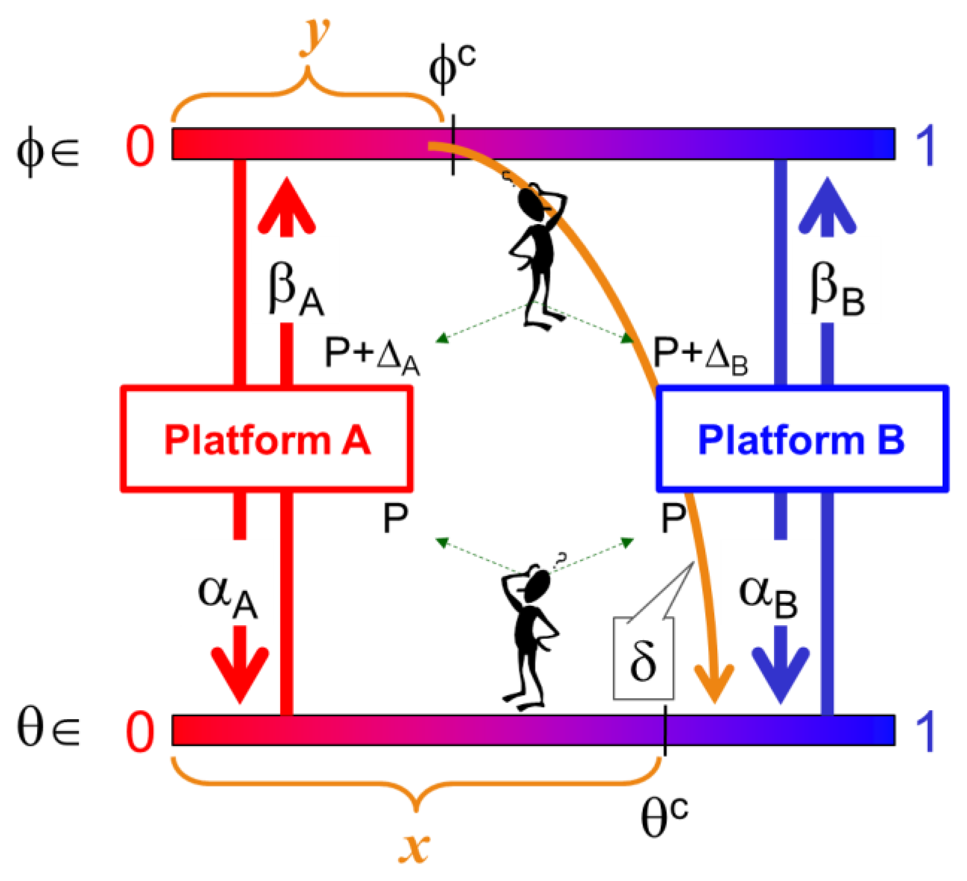
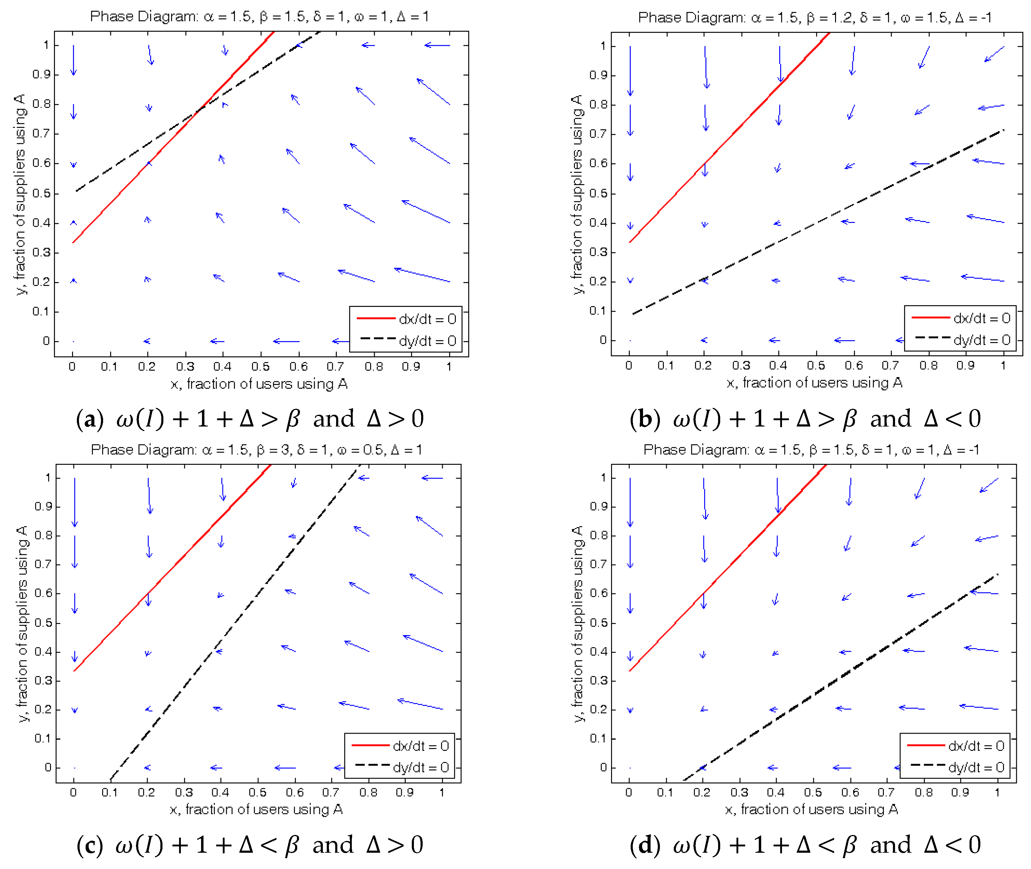
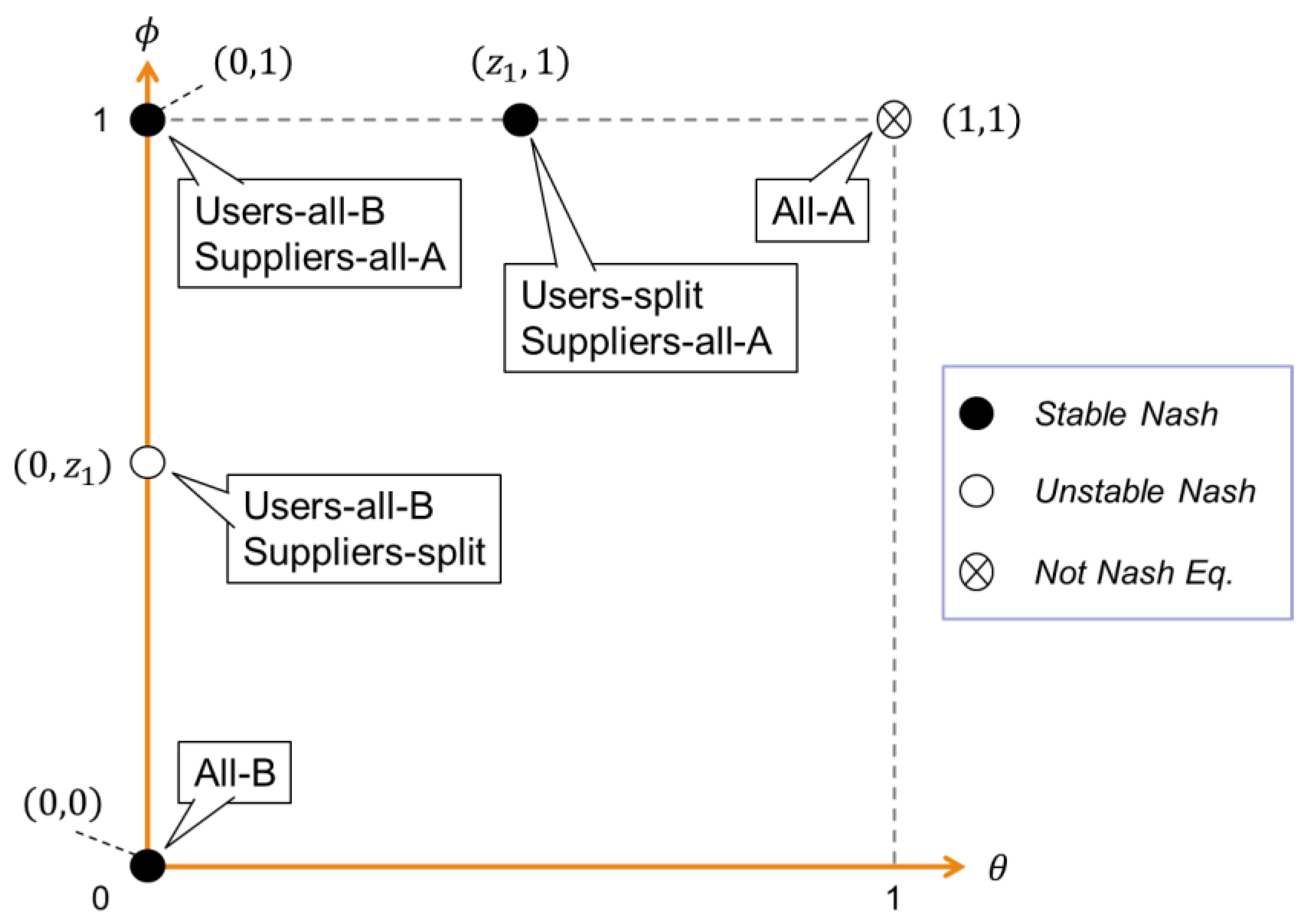
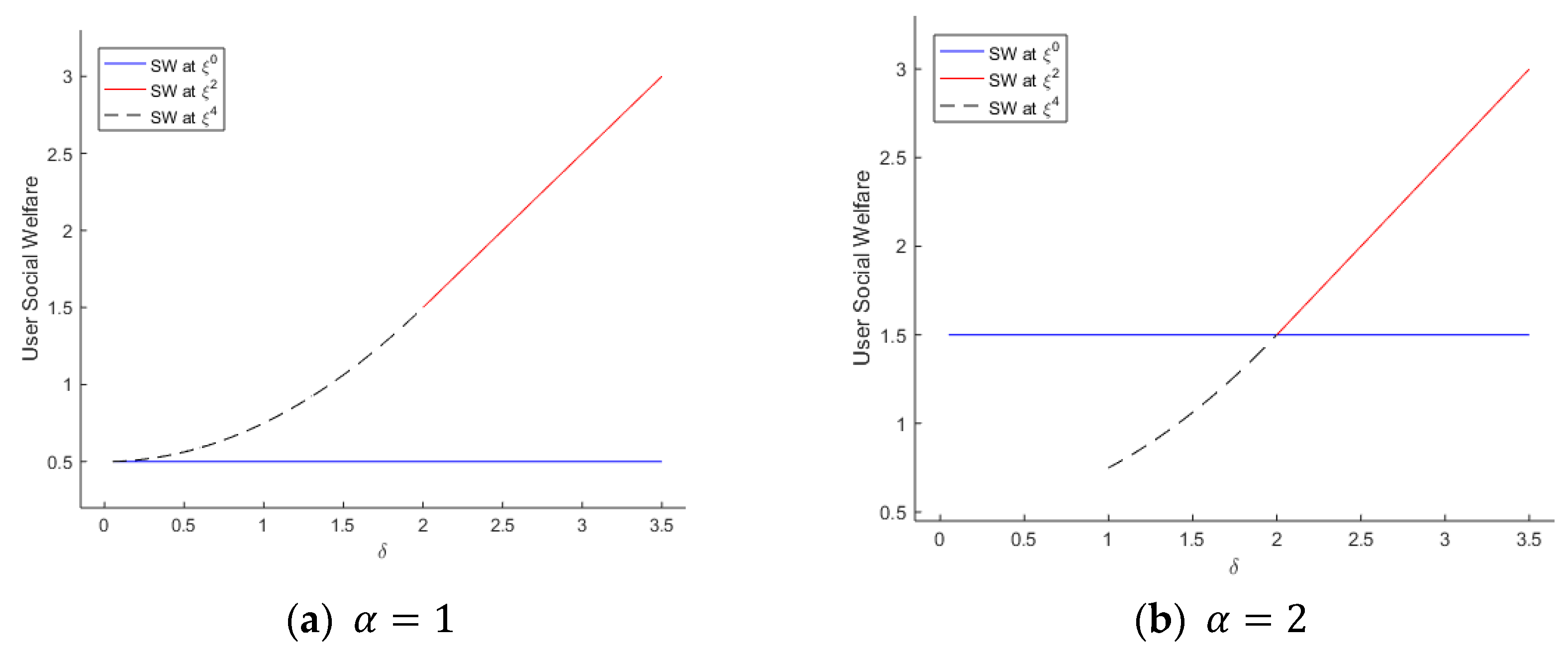
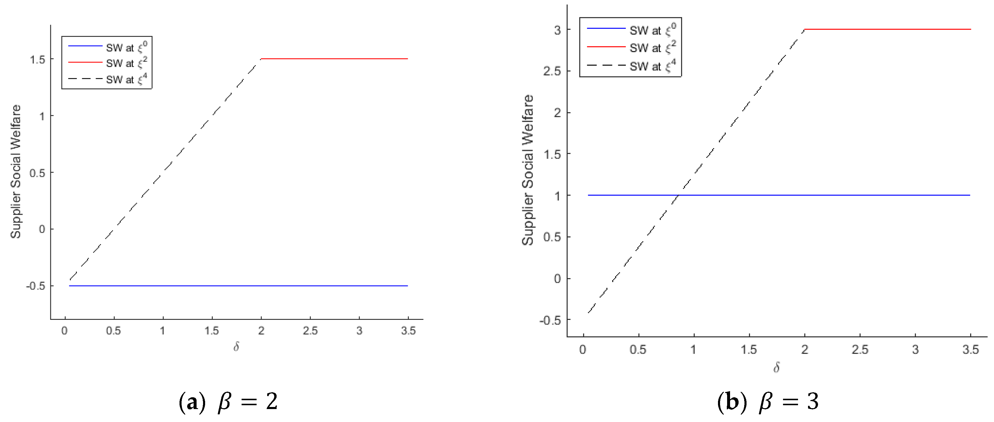
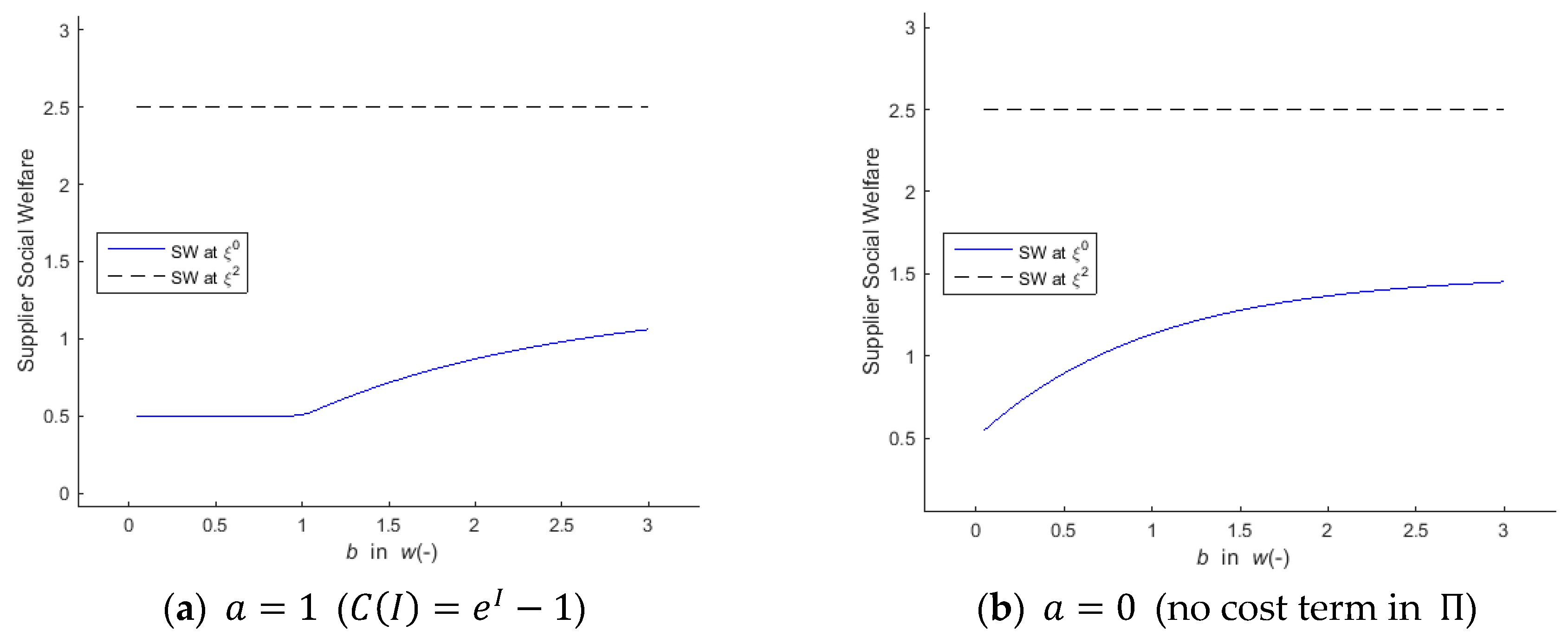
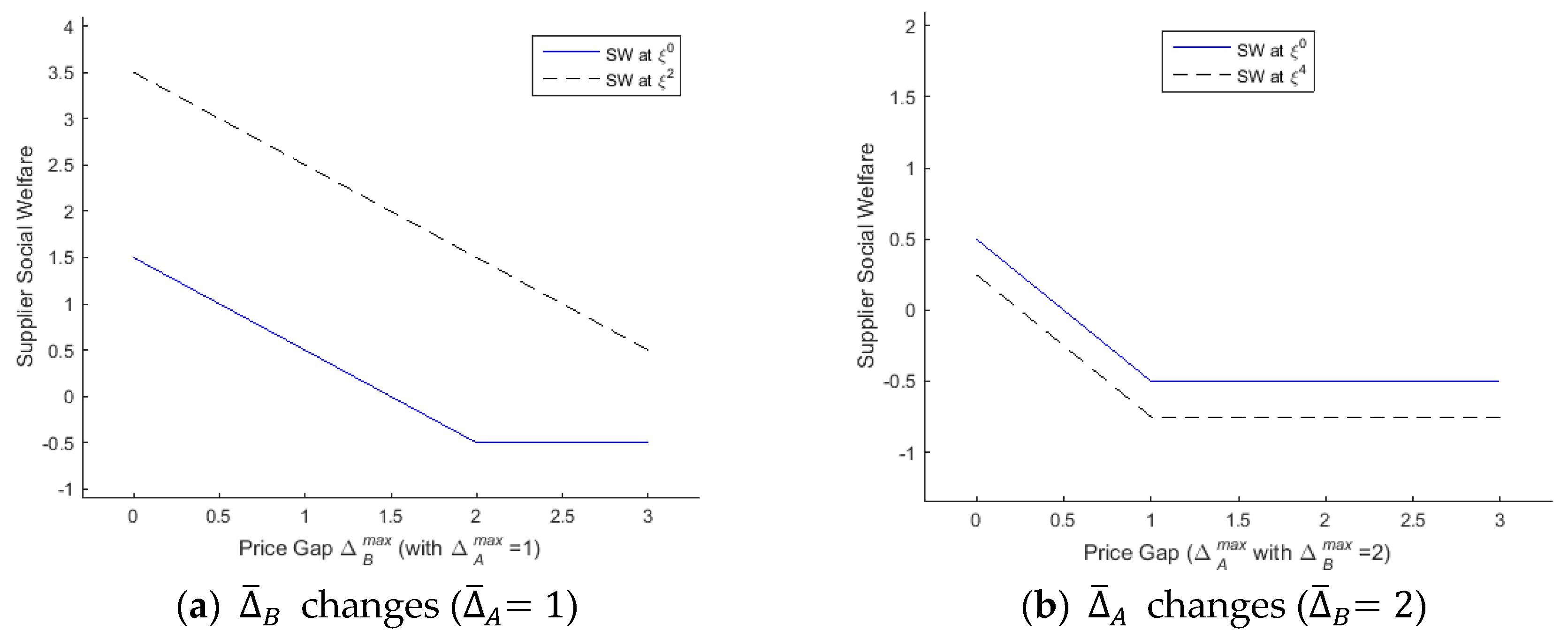
Table 1.
Platform provider’s payoffs in scenarios.
| Scenarios | Platform Provider’s Profits | |
|---|---|---|
| Scenario I | ⓐ | ⓑ |
| ( at ) | ( at ) | |
| Scenario II () | ||
| Scenario III () | ||
© 2018 by the author. Licensee MDPI, Basel, Switzerland. This article is an open access article distributed under the terms and conditions of the Creative Commons Attribution (CC BY) license (http://creativecommons.org/licenses/by/4.0/).
Share and Cite
MDPI and ACS Style
Kim, D. Equilibrium Analysis for Platform Developers in Two-Sided Market with Backward Compatibility. Games 2018, 9, 76. https://doi.org/10.3390/g9040076
AMA Style
Kim D. Equilibrium Analysis for Platform Developers in Two-Sided Market with Backward Compatibility. Games. 2018; 9(4):76. https://doi.org/10.3390/g9040076
Chicago/Turabian StyleKim, Dohoon. 2018. "Equilibrium Analysis for Platform Developers in Two-Sided Market with Backward Compatibility" Games 9, no. 4: 76. https://doi.org/10.3390/g9040076
Note that from the first issue of 2016, this journal uses article numbers instead of page numbers. See further details here.