Article

Prescriptive Norms and Social Comparisons

1
Department of Economics, University of Haifa, Haifa 3498838, Israel
2
Department of Economics, Uppsala University, SE-751 05 Uppsala, Sweden
3
Oslo Business School, Oslo Metropolitan University, NO-0130 Oslo, Norway
*
Author to whom correspondence should be addressed.
Games 2018, 9(4), 97; https://doi.org/10.3390/g9040097
Submission received: 22 August 2018 / Revised: 28 October 2018 / Accepted: 23 November 2018 / Published: 5 December 2018
(This article belongs to the Special Issue Social Norms and Games)

Abstract

:
This paper analyzes the equilibrium strength of prescriptive norms to contribute to public goods. We consider three methods of establishing what an acceptable contribution to the public good is. Under the first method, the contribution of the bottom contributor is the reference point by which the comparison is being made; under the second, the median contribution is the reference point; and under the third the top contribution is the reference. The first method results in a unique equilibrium and the reference contribution is endogenously low. Each of the latter two methods allows for multiple equilibria differing in contributions made and thus in the strength of the norm to contribute. Comparing the methods we show that the median reference allows for the highest equilibrium contributions and welfare of all methods hence is the preferred method if, among the multiple equilibria, the best one can be selected. However, the bottom-reference is the maximin method, i.e., it provides safe minimal aggregate contribution and welfare that surpass the worst outcome in the other two methods.
JEL Codes:
D02; D90; H41; Z1

1. Introduction

Imagine an individual who considers contributing to a public good in a setting where high contributions are socially rewarded. How will this individual’s contribution be affected by the reference point that is being used to determine what is a socially acceptable contribution? And how will the reference point itself change by the contribution of this and other individuals? This paper analyzes the strength of such social norms and how it is affected by which social comparison is being used to judge what is considered a socially acceptable contribution. By the “strength of a norm to contribute” we refer to the stigma associated with not contributing—a stronger norm to contribute implies a higher loss of social esteem when shirking from contribution.
Social norms can be divided into two main categories: descriptive and prescriptive (Cialdini et al. [1]). A descriptive norm, also referred to as a convention, refers to an action that is “commonly done” (Cialdini et al. [1], p. 202). Hence its very existence is contingent on agents in society behaving according to it.1 Prescriptive (or injunctive) social norms, which are the focus of this paper, describe a “commonly approved” behavior (Cialdini et al. [1], p. 202; see also Krupka and Weber [8]). Typical examples of such behavior are working hard, not littering or polluting, being polite, donating to charity, paying taxes or more generally contributing to a public good. These situations are characterized by positive externalities where if one agent contributes more to the public good other agents are better off. Hence, the normatively prescribed behavior is that the more one contributes the better it is. Furthermore, due to the positive externalities, a prescriptive norm (unlike conventions) may have some bite despite not being fully followed by many in practice. For example, in public-good settings, high contributions are commonly approved even when contributions are low. However, as has been documented empirically, the incentive of a single player for contributing (and equivalently, the social sanctioning for not) is affected by the contributions of the others.2
Based on this description, we present a public-good game with two main properties: a player gets a social reward that is increasing in her contribution;3 and the social incentive to contribute is increasing in what other players do.4 In this setting we analyze how the mechanism for social comparison of what constitutes a socially acceptable contribution affects contributions in equilibrium. More precisely we consider three modes of social comparison. In the first, the contribution of the bottom contributor is the reference point and contributions above it are rewarded. In the second, the top contributor is the reference point and contributions below are sanctioned. In the third, the median contributor constitutes the reference and contributions above are rewarded and below are sanctioned.5 We analyze the existence of multiple equilibria, the distribution of contributions among the players and the total contribution and welfare in these equilibria and show how the equilibrium properties depend on the social-comparison method used.
There is a robust empirical observation in public-good settings, that information about what others contribute has an effect on individual contributions [22,23,24,25,26]. In these lab and field experiments, information typically comes in the form of a reference point essentially saying “this is how much others contributed on average” or “this is how much a random person contributed”. In particular, they show that high reference points tend to increase contributions while low reference points decrease contributions—a feature present in our model too. There is also a series of papers (see, for instance, Clark and Oswald [21], Festinger [27], Sugden [28], Brekke et al. [29], Fehr and Gächter [30], Herrmann et al. [31]) which analyze (either theoretically or experimentally) the effect of a reference point on contributions. However, each such paper looks at only one reference point (typically the average or median contribution). No previous paper has systematically compared which form of reference point yields the highest contributions. This is the main purpose of our paper. It is important, since it informs, in particular for smaller groups, which information should be presented to participants. Alternatively, our results can be interpreted in terms of choosing which institution is best at overcoming the free-rider problem in public-good settings. These issues are discussed, in light of the results we find, in the conclusions.

2. Model

Three players play a linear public good game: each player i = 1 , 2 , 3 chooses how many units x i R 0 + to contribute to the public good, and the sum of contributions is multiplied by a productivity coefficient a 1 , 3 and then equally divided between the three players. Beyond this material payoff, players gain a (possibly negative) social esteem S R , depending on the deviation from some endogenously determined reference point x r . The utility of player i is thus given by
u i = a 3 j i x j 1 a / 3 x i + S x i x r ,
where
S x i x r = f x i x r if x i x r 0 f x r x i if x i x r < 0 .
That is, contributing more than x r yields an esteem of f Δ x i x i x r , where f Δ x i is assumed to be twice differentiable for Δ x i > 0 with f Δ x i > 0 and f Δ x i < 0 , and f 0 = 0 . The setting is meant to reflect that the strength of the norm to contribute is increasing in the reference point. Formally this is captured by the social esteem when contributing zero, S 0 x r , being decreasing in x r . The social esteem function is depicted in Figure 1. The properties of f imply that surpassing the reference point by a little yields a high increase in social esteem but that the marginal increase in social esteem fades off when surpassing it more.6 Contributing less than x r yields a loss of esteem that is equivalent to the gain when surpassing the reference. Hence, as when surpassing the reference, the social esteem changes a lot when contributing slightly below the reference but the marginal effect fades when further undercutting the reference. This way the gains and losses are normalized to the reference point, whatever it is.7
The three players choose their contributions simultaneously, hence each player takes the contributions of the others as given when evaluating the best response. Define k 1 a / 3 . Player i then chooses x i to maximize
v i k x i + S x i x r .
We are interested in how the method of social comparison affects the players’ decisions how much to contribute. We will hence let the reference point be determined in three alternative ways. In the first, the reference point equals the contribution of the bottom contributor: x r = m i n x i . In the second, the reference point equals the contribution of the top contributor: x r = m a x x i . In the third, the reference point equals the contribution of the median contributor: x r = m e d i a n x i . It should be noted that the particular player who ends up taking the role of reference-point setter is in itself an equilibrium outcome. The norm is thus set simultaneously with all players’ contribution choices, and an equilibrium holds when all players are best responding to the endogenously determined norm. In particular, we will focus on pure-strategy equilibria and impose three further restrictions on f. First, the concavity of f Δ x implies that if f 0 k then the equilibrium is degenerate: x i = 0 i . Hence, to make the problem interesting, the first restriction is (i) f 0 > k . Second, we require (ii) lim Δ x f Δ x < k to ensure that equilibrium contributions are finite. Finally, noting that under these two conditions there is a (unique) solution to f Δ x = k in the range Δ x > 0 , denoted hereafter by Δ x * , we require (iii) f Δ x * Δ x * 2 k , since otherwise (as will be clear from the proofs) no pure-strategy equilibrium exists.8

3. Equilibrium Contributions Under Each Social Comparison Method

3.1. Bottom-Contributor Comparison

Suppose x r = m i n x i so that the lowest contribution among the players is the reference point. A pure strategy profile X = x i i = 1 , 2 , 3 is a Nash Equilibrium (NE) if no player has a profitable deviation given the strategies of the other two players.
Proposition 1.
Let x r = m i n x i . Then there exists a unique pure-strategy NE. In this equilibrium, x r = m i n x i = 0 and m e d i a n x i = m a x x i = Δ x * > 0 .
The intuition for the proposition is as follows. Since the reference point moves together with the choice of the bottom contributor, this player can gain no social esteem by increasing the contribution—as long as she stays the bottom contributor—and can only hope to save on material costs of contribution. This implies that, if the equilibrium exists, the bottom contribution and hence the reference necessarily has to be zero. Given this choice of the bottom contributor, the two other players are better off choosing to contribute more (recall that there is a high increase in social esteem when surpassing the reference point while the cost of contributing increases linearly). How much more? There is a unique value Δ x * where the marginal cost of contribution equals the marginal benefit, so this will be their choice. Given this choice, the bottom contributor will not try to “pass” the other two under the condition f Δ x * Δ x * 2 k which is what was assumed under restriction (iii).9 We will see below that using each of the other two comparison methods has the potential of increasing the total contribution to the public good.10

3.2. Top-Contributor Comparison

Now suppose x r = m a x x i so that the highest contribution among the players is the reference point.
Proposition 2.
Let x r = m a x x i . A strategy profile is a pure-strategy NE iff x r [ 0 , x ^ ] and m i n x i = m e d i a n x i = m a x x i = x r , where x ^ is the unique solution to the equation f x = k x .11
The intuition for the proposition is as follows. Given the contributions of the other two, the top contributor would only lose by increasing her contribution above that of the median. This is so because any such increase implies a higher material cost with no increase in social esteem, given that the top contributor herself sets the criterion. Hence, the two highest contributors contribute the same in any equilibrium. Of course, the top contributor may consider going below the current median but then the role of top contributor moves to the previous median and the same logic of no benefit from surpassing the median holds again. The bottom contributor might profit from contributing less than the other two. However, in that case, the current median would also profit by imitating the bottom contributor (as they compare themselves to the same reference point—the top contributor). Thus, in equilibrium, the bottom and the median contributor must choose the same x i (unless they are precisely indifferent, as mentioned in the footnote of the proposition). In total, all players thus contribute the same in equilibrium. When this is the case, by the logic of it being pointless to push the reference point further, a profitable deviation can only be to contributing less than the reference. In particular, given the convexity of f Δ x when contributing less than the reference point, once one deviates slightly below the reference point further deviations are not that costly. This has two implications. The first is that the choice boils down to contributing either precisely the same as the reference point or contributing zero. The second implication is that contributing zero becomes increasingly attractive as the reference point increases. This is because the cost of contributing is linear (so that matching the reference point becomes increasingly costly when the reference point increases) while the loss of esteem is increasing concavely when contributing zero and the reference point increases.12 This means that there will exist an upper limit for the reference point in equilibrium. This is x ^ . However, there exist multiple equilibria, each one defined by a specific reference point below x ^ , implying that we may observe either high or low contributions in equilibrium or, put differently, that the strength of the prescriptive norm to contribute may be either high or low.13

3.3. Median-Contributor Comparison

Finally, suppose x r = m e d i a n x i so that the median contribution is the reference point.
Proposition 3.
Let x r = m e d i a n x i . A strategy profile is a pure-strategy NE iff x r [ 0 , x ^ ] , m i n x i = m e d i a n x i = x r and m a x x i = x r + Δ x * .
The proposition says that the two lowest contributors will contribute the same. The intuition for this is that the median has no reason to contribute more than the bottom contributor as this would imply increased material costs with no gain in social esteem as the reference point moves along with the median contribution. Of course, if the median would contribute less than the bottom contributor then the roles would change and the median would herself become the bottom contributor and the logic would then apply to the “new median”. Given the contribution of the median, the top contributor will choose to contribute strictly more than the median. The reason is that f is concave implying that surpassing the median even slightly comes with a high social reward. On the other hand, again due to the concavity of the social esteem of surpassing the median, there is no point in surpassing it by a lot. This implies the top contributor has an intermediate solution which is given by x r + Δ x * . The top contributor may of course consider deviating to contributing below the median. Due to the large social loss of contributing just below the reference point ( f is convex), the most tempting deviation considered by the top contributor would be to contributing zero. The zero point becomes relatively more attractive the higher is x r since the alternative choice, of surpassing a high reference point, comes at a higher material cost while not giving a higher social esteem than if x r were low. This is the first reason why the equilibrium reference point has to be sufficiently small—otherwise the top contributor would deviate. The second reason is that, if x r is high, then the bottom contributor (who in equilibrium emulates the median) would deviate to zero. Emulating the median is relatively more costly when the median contributes a lot (due to linearity of the material cost and the convexity of f ), and this sets an upper bound on the reference point.14 Preventing the bottom contributor from deviating to zero implies a stricter constraint on x r than preventing the top contributor from deviating to zero. The reason for this is that ultimately, in equilibrium, the top contributor is better off than the median and bottom contributor (otherwise the top contributor could simply emulate the median), therefore the top contributor is always less inclined than the other two to deviate to zero. Hence, as expressed in the proposition, there is only one constraint on the maximum value of x r . This constraint is the same as when the top-contribution is the reference point (Section 3.2) and is given by x r x ^ . Any value below x ^ is sustainable in equilibrium implying that there exist multiple equilibria.15

4. Comparing the Social-Comparison Methods

We will now compare the results of the different social-comparison methods in terms of contributions and in terms of welfare ( i u i from Equation (1)), where the latter includes also the social esteem component. We will first present results considering the payoff-dominant equilibria and then present maximin criteria for comparison.
Proposition 4.
(i) The pure-strategy NE with the highest total contribution is achieved under median-contributor comparison; (ii) If the productivity coefficient a is sufficiently high ( a 9 / 7 ) then the pure-strategy NE with the highest total welfare is achieved under median-contributor comparison, while if it is sufficiently low ( a 1 + ) then the pure-strategy NE with the highest total welfare is achieved under the bottom-contributor comparison.
Before discussing and explaining the results, note first that given that the underlying setting is a public good game, higher contributions result in higher welfare when fixing the relative contributions (and consequently the social esteem of the players). Thus, when equilibrium contributions are determined with respect to a reference point x r (like in Propositions 2 and 3), higher values of x r imply both higher contributions and higher welfare.
To see the intuition for the results in Proposition 4, note that both the median- and the top-contributor comparison methods allow for multiple equilibria with x r x ^ . In that sense these methods of social comparison are similar and allow for different equilibrium strengths of the prescriptive norm. However, under the median-contributor comparison method, one player always contributes x r + Δ x * while under the top-contributor comparison method all players contribute x r . Thus, given a reference point x r , the total contribution is higher under the median-contributor comparison method than under the top-contributor comparison method. Given that by deviating upwards by Δ x * the top contributor increases both her contribution and her social esteem (without affecting the esteem of others, given that the reference point—the median contribution—is unchanged), total welfare is also higher under the median-contributor comparison method than under the top-contributor comparison method. As explained earlier, in both these methods the total contribution and welfare are maximized when x r = x ^ , in which case the bottom contributor (who contributes x r = x ^ ) contributes still more than the top contributor under the bottom-contributor comparison method (who contributes Δ x * ; see the proof of the proposition as to why x ^ > Δ x * ). Hence, the highest possible total contribution is achieved under median-contributor comparison (result (i)).
Given the logic sketched above, welfare can be maximized only under either the median- or the bottom-contributor comparison methods. The sum of utilities under the median-contributor comparison method (with x r = x ^ ) by equation (1) is a 1 i x i + i S x i x r = a 1 3 x ^ + Δ x * + f Δ x * . The sum of utilities under the bottom-contributor comparison method is 2 a 1 Δ x * + 2 f Δ x * . The difference between the sums is hence given by
a 1 3 x ^ Δ x * f Δ x * .
This expression is negative for a 1 + (where it approaches f Δ x * < 0 ) and positive for any a 9 / 7 .16 More intuitively, the strength of the bottom-contributor method is that it yields the players a high aggregate social esteem since two players surpass the reference, while in the median method only one player surpasses the reference. On the other hand, the strength of the median-contributor method is that it yields higher contributions in equilibrium, in particular when x r = x ^ . Hence the median method achieves the highest attainable welfare when the public-good multiplier a is high, so that high contributions are important for aggregate welfare, while the bottom method achieves the highest welfare of all methods when the public-good multiplier is low so that social esteem is more important for aggregate welfare. This explains result (ii).
Another relevant equilibrium-selection criterion—which focuses on the highest floor rather than the highest upside—is that of maximin.
Definition 1.
A social-comparison method is a maximin-contribution method if, when comparing (across the three methods) the pure-strategy NE thatminimizetotal contribution under each method, this method generates the highest contributions. An equivalent definition applies to a maximin-welfare method.
Proposition 5.
The bottom-contributor comparison method is both the maximin-contribution method and the maximin-welfare method.
This result follows from the fact that the bottom-contributor comparison method allows for only one equilibrium – one where the reference point is zero. This would suggest low contributions. However, as mentioned above, under this method two of the players contribute more than the reference (more precisely they contribute Δ x * ) while under the median-contributor comparison method only one player surpasses the reference (and under the top-contributor comparison method no one surpasses the reference). As explained earlier, the worst case scenario (in terms of contribution and, consequentially, welfare) under the median- and the top-contributor comparison methods is when x r = 0 , in which case the total contribution is only Δ x * under the median-contributor comparison method (and 0 under the top). This is compared to a total contribution of 2 Δ x * under the bottom-contributor comparison method. This explains Proposition 5.17

5. Conclusions

This paper has analyzed the endogenous strength of prescriptive norms and how it depends on the method of comparison used to determine what a socially acceptable level of contribution to a public good is. We consider three methods of comparison: (1) the contribution of the bottom contributor is the reference point determining social reward and sanctioning; (2) the contribution of the top contributor is the reference point; and (3) the contribution of the median contributor is the reference point.
When the median or top contributors constitute the reference of comparison then the prescriptive norm may take on different strengths—there exist multiple equilibria. These equilibria differ in how high the endogenous reference contribution is. Furthermore, while the highest attainable reference contribution is the same under both the median and top reference methods, the maximal total contribution is the highest when the median is the point of comparison. Thus, using the median as a comparison allows for a higher welfare than using the top as a reference. When the bottom contributor constitutes the reference of comparison, the equilibrium is unique and the reference is necessarily low (zero). Nevertheless, despite this reference point being low, both the maximal contribution and the aggregate contributions may be higher than under the two other comparison methods (in case the players fail to coordinate on a sufficiently high contribution level in these methods). Thus, using the bottom contributor as a reference is a safe way of ensuring a minimal aggregate contribution and welfare in equilibrium. Moreover, when the productivity coefficient of the public good is particularly low, this method also maximizes welfare (through the channel of social esteem).
Our analysis has both positive and normative implications. Positively, we provide predictions for how groups—differing in the reference point they use, which is a form of institution—would differ in their distribution of contributions. One prediction is that groups using the median or top contributor methods will have a higher variance of contributions (since they allow for multiple equilibria) compared to groups using the bottom-contributor method. Another prediction is that groups using the median-contributor method allow for the highest total contribution. Furthermore, groups using the bottom-contributor method are expected to have a higher low bound on the total contribution.
Normatively, our results have bearing to the extent that one can affect the institution of social comparisons. Our results provide a theoretical underpinning for the literature testing the effect of information about others’ contributions on the individual’s contribution [22,23,24,25,26]. In particular, we highlight which information would allow for the highest contributions in equilibrium. These normative implications can be empirically tested in similar settings as the ones studied by the research just mentioned (e.g., energy conservation and campaign contributions). In particular, our results capture the drawback of comparing people’s contributions to the top contributor. While it may be tempting to use the highest standard as a reference point, it may backfire when considering the equilibrium effects: it discourages the top contributor from excelling further and thus keeps everyone back. This has an interesting and somewhat surprising policy implication: although it is quite customary (in fundraising for example) to highlight the top contribution, our model implies that a better strategy is to rather highlight the median contribution or even, in some cases, the bottom contribution.
Naturally, there may be other aspects to social comparison not captured by our analysis, for instance, what happens dynamically if the person that happens to currently be the reference point is rewarded. Hence, there are interesting avenues for extending the analysis presented here.

Author Contributions

Both authors have contributed equally to all aspects of this work.

Funding

This research was funded by Jan Wallander’s och Tom Hedelius’ foundation grant number P18-0142.

Conflicts of Interest

The authors declare no conflict of interest. In particular, the founding sponsors had no role in the analyses and in the decision to publish the results.

Appendix A. Proofs

Appendix A.1. Proof of Proposition 1

Proof. 
Given that x r = m i n x i , f x i x r = 0 for the bottom contributor. Suppose now by negation that m i n x i 0 . Then, by deviating to a smaller value of x i , the player who chooses m i n x i reduces her cost of contribution k x i while not affecting f x i x r . Thus this is a profitable deviation, hence, in equilibrium, it must be that m i n x i = 0 . Given that, by restriction (i), v 0 = k + f ( 0 ) > 0 , none of the other two players will choose x i = 0 . In particular, due to restrictions (i) and (ii) both players have a unique inner solution at Δ x * > x r = 0 where f Δ x * = k . Finally, the player choosing m i n x i must not have a profitable deviation to contributing more. Given the concavity of f x for values above the reference point and its convexity below, such a deviation, if it exists, will be to x i = 2 Δ x * , because the inner local max point of the player’s optimization problem is achieved at distance Δ x * above the choice of the others (who, by this deviation, become the bottom contributors), and the others were shown to choose Δ x * . This is not a profitable deviation iff v 0 v 2 Δ x * , i.e., if 0 f Δ x * 2 k Δ x * , which holds by restriction (iii). □

Appendix A.2. Proof of Proposition 2

Proof. 
IF: Suppose m i n x i = m e d i a n x i = m a x x i = x r [ 0 , x ^ ] . First note that, given that m a x x i sets the reference point, no player can have a profitable deviation to contributing more than the others, because this would strictly increase the cost of contribution without increasing the social esteem. Next note that, given that S is convex for contributions below the reference point, a profitable deviation to below the reference (if it exists) would be to choosing x i = 0 . Hence, a player would deviate iff v 0 > v x r f x r < k x r x r > x ^ .
IF for the case in the footnote: Suppose m i n x i = 0 and m e d i a n x i = m a x x i = x r = x ^ . We just established that no player would deviate to contributing strictly more than the others and that the only best responses weakly below the reference point are either 0 or x r . Here all players are indifferent between 0 and x r = x ^ because none of the deviations considered will change the reference point and since v 0 = v x r f x r = k x r x r = x ^ . Hence, no one deviates.
ONLY IF: First, suppose m e d i a n x i < m a x x i = x r . Then the top contributor has a profitable deviation to contributing the same as m e d i a n x i , because this would decrease the top contributor’s cost of contribution k x i while not affecting her social esteem. Thus, m e d i a n x i = m a x x i = x r must hold in equilibrium. Second suppose m e d i a n x i = m a x x i = x r > x ^ . Then, one of these players would deviate to zero because the reference point would remain the same and v 0 > v x r f x r < k x r x r > x ^ . Thus, m e d i a n x i = m a x x i = x r x ^ must hold in equilibrium. Third suppose m i n x i x b < x m m e d i a n x i = m a x x i = x r x ^ . The bottom contributor does not have a profitable deviation if either her payoff when choosing x b is strictly higher than when choosing x m , which implies (by the fact that both the median and bottom contributors use the same reference) that also the median is better off choosing x b (i.e., the median has a profitable deviation); or, alternatively, the bottom and median contributors are indifferent between x b and x m = m a x x i = x r . It was shown above (under “IF for the case in the footnote”) that these strategies are part of an equilibrium if x b = 0 and x m = m a x { x i } = x r = x ^ . So here we have to show that it is not an equilibrium if either x b 0 or x m x ^ . Since S is convex below the reference point, v i is convex for contributions below the reference. Hence, either x b > 0 , in which case the bottom player would have a profitable deviation to 0, in contradiction to x b being her equilibrium strategy; or x b = 0 , in which case the indifference between x b = 0 and x m = x r implies that v 0 = v x r f x r = k x r x r = x ^ which contradicts x m = m a x { x i } = x r x ^ . □

Appendix A.3. Proof of Proposition 3

Proof. 
IF: Suppose x r [ 0 , x ^ ] and m i n x i = m e d i a n x i = x r ; m a x x i = x r + Δ x * . First, the top contributor cannot do better than x r + Δ x * while staying (weakly) above x r , due to her optimization problem as given in Equation (3). Next, a deviation of any one of the three players to x i < x r would not change the reference point and could only be to zero, given that S is convex for contributions below the reference point. This deviation is not profitable for the two bottom contributors if v 0 v x r f x r k x r x r x ^ , in which case it is also not profitable for the top contributor, for whom the same values of v 0 and v x r apply and, in addition, it was just shown that v x r < v x r + Δ x * . Thus, the top contributor has no profitable deviation and the bottom two contributors have no downward profitable deviation. Finally, an upward deviation of any of the two bottom contributors to x i x r , x r + Δ x * would imply a higher cost of contribution without changing the social esteem (because the deviator stays the median contributor hence the reference point); and an upward deviation of any of the two bottom contributors to x i > x r + Δ x * changes the role of the current top contributor from top to median contributor, thereby changing the reference point to be x r + Δ x * . If any of the two bottom contributors indeed deviates to contributing above this point, the best she could do is to contribute x r + 2 Δ x * (given her optimization problem with respect to a reference point at x r + Δ x * , as explained above). This would increase her cost of contribution by 2 k Δ x * while increasing her social esteem only by f Δ x * (because the reference point itself moves from x r to x r + Δ x * ). This deviation is not profitable by restriction (iii), according to which f Δ x * Δ x * 2 k .
ONLY IF: First suppose m i n x i < m e d i a n x i . Given that x r = m e d i a n x i implies f x i x r = 0 for the median contributor regardless of her contribution, any strategy profile with m i n x i < m e d i a n x i is not an equilibrium—the median has a profitable deviation to contributing exactly like the bottom contributor because this would strictly decrease the cost of contribution without affecting the esteem. Second note that the top contributor necessarily contributes x r + Δ x * because, in the range where the top contributor can be (i.e., weakly above x r ), this contribution maximizes her utility as given in equation (3). Thus, we have shown that in equilibrium it must be that m i n x i = m e d i a n x i = x r and m a x x i = x r + Δ x * . The only thing left to show is that x r , the contribution of the two bottom players, must be x ^ . This follows immediately from the fact that any of these two players would have a profitable deviation if v 0 > v x r f x r < k x r x r > x ^ . □

Appendix A.4. Proof of Proposition 4

Lemma A1.
For any distribution of contributions that is fixed relative to the reference point x r , increasing x r results in increased welfare.
Proof. 
Given that contributions are fixed relative to x r , the social esteem of each player is fixed, and so welfare changes only as a function of changes in the contributions following a change in x r . Then, an increase in x r results in an increase of the contributed sum by 3 a at a cost of 3, i.e., an increase of material (hence also total) welfare by 3 a 1 , which is positive by assumption. □
Lemma A2.
Δ x * < x ^ .
Proof. 
Δ x * is the point where f Δ x = k in the range Δ x > 0 , while x ^ is the solution to the equation f x = k x . Given that f · is concave, the average slope in the range 0 , Δ x * is larger than k, implying that f Δ x * Δ x * > k , hence (again by concavity) we get that Δ x * < x ^ . □

Appendix A.4.1. Proof of the proposition

Proof. 
(i) Given that under both the median- and the top-contributor comparison methods x r can take any value in the range 0 , x ^ , the total contributions are highest when x r = x ^ . Then, since under the median-contributor comparison method the top contributor contributes x r + Δ x * , this method yields the equilibrium with the highest contributions among these two methods. Under the bottom-contributor comparison method the total contribution is 2 Δ x * , which by Lemma A2 falls short of 3 x ^ + Δ x * , the highest contribution under the median-contributor comparison method.
(ii) It it immediate that, under both the median- and the top-contributor comparison methods, contributions are minimal when x r = 0 . In that case the total contribution is Δ x * under the median-comparison method and 0 under the top-contributor comparison method, compared to 2 Δ x * under the bottom-contributor comparison method. As for welfare, given that this case also minimizes welfare (by Lemma A1) and that in this case x r = 0 for all three methods, also the welfare is maximized under the bottom-contributor comparison method (where it equals f 0 + 2 f Δ x * = 2 f Δ x * , compared to f Δ x * and 0 under the other two methods).
(iii) For any given x r [ 0 , x ^ ] , welfare is higher under the median-contributor comparison method than under the top-contributor comparison, because the contribution of the top contributor above x r in the former method increases both the aggregate material utility (by a 1 Δ x * ) and the esteem-related utility (by f Δ x * ). We thus need to compare only the equilibrium with the highest total welfare under the medium-contributor comparison method (i.e., given Lemma A1, the one where x r = x ^ and contributions from small to large are x ^ , x ^ , x ^ + Δ x * ) with the (unique) equilibrium under the bottom-contributor comparison (in which contributions from small to large are 0 , Δ x * , Δ x * ). The difference in welfare is then given by (4). If a 1 + this difference approaches f Δ x * < 0 , hence welfare is higher under the bottom-contributor comparison method. If a 9 / 7 we get by Lemma A2 and by the monotonicity of f · that Δ x * < x ^ f Δ x * < f x ^ = k x ^ = 1 a / 3 x ^ , implying that the welfare difference given by (4) is greater than a 1 3 x ^ Δ x * 1 a / 3 x ^ > 2 a 1 x ^ 1 a / 3 x ^ = 7 3 a 3 x ^ 0 . □

References

  1. Cialdini, R.B.; Kallgren, C.A.; Reno, R.R. A focus theory of normative conduct: A theoretical refinement and reevaluation of the role of norms in human behavior. In Advances in Experimental Social Psychology; Academic Press: Cambridge, MA, USA, 1991; Volume 24, pp. 201–234. [Google Scholar]
  2. Schelling, T.C. The Strategy of Conflict; Harvard University Press: Cambridge, MA, USA, 1960. [Google Scholar]
  3. Lewis, D.K. Convention: A Philosophical Study; Harvard University Press: Cambridge, MA, USA, 1969. [Google Scholar]
  4. Granovetter, M. Threshold Models of Collective Behavior. Am. J. Sociol. 1978, 83, 1420–1443. [Google Scholar] [CrossRef]
  5. Young, H.P. The Evolution of Conventions. Econometrica 1993, 61, 57–84. [Google Scholar] [CrossRef]
  6. Michaeli, M.; Spiro, D. From Peer Pressure to Biased Norms. Am. Econ. J. Microecon. 2017, 9, 152–216. [Google Scholar] [CrossRef]
  7. Carvalho, J.P. Coordination and culture. Econ. Theory 2017, 64, 449–475. [Google Scholar] [CrossRef]
  8. Krupka, E.L.; Weber, R.A. Identifying social norms using coordination games: Why does dictator game sharing vary? J. Eur. Econ. Assoc. 2013, 11, 495–524. [Google Scholar] [CrossRef]
  9. Cialdini, R.B. Crafting normative messages to protect the environment. Curr. Directi. Psychol. Sci. 2003, 12, 105–109. [Google Scholar] [CrossRef]
  10. Blumenthal, M.; Christian, C.; Slemrod, J.; Smith, M.G. Do normative appeals affect tax compliance? Evidence from a controlled experiment in Minnesota. Natl. Tax J. 2001, 54, 125–138. [Google Scholar] [CrossRef]
  11. Booij, A.S.; Leuven, E.; Oosterbeek, H. Ability peer effects in university: Evidence from a randomized experiment. Rev. Econ. Stud. 2017, 84, 547–578. [Google Scholar] [CrossRef]
  12. Young, H.P. Social norms and economic welfare1. Eur. Econ. Rev. 1998, 42, 821–830. [Google Scholar] [CrossRef]
  13. Jackson, M.O.; Zenou, Y. Games on networks. In Handbook of Game Theory with Economic Applications; Elsevier: Amsterdam, The Netherlands; New York, NY, USA, 2015; Volume 4, pp. 95–163. [Google Scholar]
  14. Nyborg, K. Social Norms and the Environment. Annu. Rev. Resour. Econ. 2018, 10, 405–423. [Google Scholar] [CrossRef]
  15. Bénabou, R.; Tirole, J. Incentives and Prosocial Behavior. Am. Econ. Rev. 2006, 96, 1652–1678. [Google Scholar] [CrossRef] [Green Version]
  16. Bénabou, R.; Tirole, J. Laws and Norms; Discussion Paper Series 6290; Institute for the Study of Labor (IZA): Bonn, Germany, 2012. [Google Scholar]
  17. Andreoni, J. Impure Altruism and Donations to Public Goods: A Theory of Warm-Glow Giving. Econ. J. 1990, 100, 464–477. [Google Scholar] [CrossRef]
  18. Harbaugh, W.T. What do donations buy?: A model of philanthropy based on prestige and warm glow. J. Public Econ. 1998, 67, 269–284. [Google Scholar] [CrossRef]
  19. Ledyard, J.O. Is there a problem with public goods provision. In The Handbook of Experimental Economics; Princeton University Press: Princeton, NJ, USA, 1995; pp. 111–194. [Google Scholar]
  20. Kandel, E.; Lazear, E.P. Peer pressure and partnerships. J. Polit. Econ. 1992, 100, 801–817. [Google Scholar] [CrossRef]
  21. Clark, A.E.; Oswald, A.J. Comparison-concave utility and following behaviour in social and economic settings. J. Public Econ. 1998, 70, 133–155. [Google Scholar] [CrossRef] [Green Version]
  22. Shang, J.; Croson, R. A field experiment in charitable contribution: The impact of social information on the voluntary provision of public goods. Econ. J. 2009, 119, 1422–1439. [Google Scholar] [CrossRef]
  23. Chen, Y.; Harper, F.M.; Konstan, J.; Li, S.X. Social comparisons and contributions to online communities: A field experiment on movielens. Am. Econ. Rev. 2010, 100, 1358–1398. [Google Scholar] [CrossRef]
  24. Rege, M.; Telle, K. The impact of social approval and framing on cooperation in public good situations. J. Public Econ. 2004, 88, 1625–1644. [Google Scholar] [CrossRef]
  25. Allcott, H. Social norms and energy conservation. J. Public Econ. 2011, 95, 1082–1095. [Google Scholar] [CrossRef] [Green Version]
  26. Frey, B.S.; Meier, S. Social comparisons and pro-social behavior: Testing “conditional cooperation” in a field experiment. Am. Econ. Rev. 2004, 94, 1717–1722. [Google Scholar] [CrossRef]
  27. Festinger, L. A theory of social comparison processes. Hum. Relat. 1954, 7, 117–140. [Google Scholar] [CrossRef]
  28. Sugden, R. Reciprocity: The supply of public goods through voluntary contributions. Econ. J. 1984, 94, 772–787. [Google Scholar] [CrossRef]
  29. Brekke, K.A.; Kverndokk, S.; Nyborg, K. An Economic Model of Moral Motivation. J. Public Econ. 2003, 87, 1967–1983. [Google Scholar] [CrossRef]
  30. Fehr, E.; Gächter, S. Cooperation and Punishment in Public Goods Experiments. Am. Econ. Rev. 2000, 90, 980–994. [Google Scholar] [CrossRef] [Green Version]
  31. Herrmann, B.; Thöni, C.; Gächter, S. Antisocial punishment across societies. Science 2008, 319, 1362–1367. [Google Scholar] [CrossRef] [PubMed]
  32. Kahneman, D.; Tversky, A. Prospect Theory: An Analysis of Decision under Risk. Econometrica 1979, 47, 263–292. [Google Scholar] [CrossRef]
1.
Theoretically, descriptive norms are typically modeled using coordination games (e.g., Schelling [2], Lewis [3], Granovetter [4], Young [5]). If an agent deviates from the actions of others then she will perceive a social pressure (or equivalently, losses of miscoordination). Examples of such settings would be choosing what side of the road to drive or, for situations where agents disagree about the preferred convention, when to have public holidays. The strength of and adherence to descriptive social norms has been studied by Michaeli and Spiro [6] and Carvalho [7].
2.
See for instance, Cialdini [9] for environmental compliance, Blumenthal et al. [10] for paying taxes and Booij et al. [11] for peer effects in educational attainment.
3.
We thus relax the strict requirement used by Young [12] who makes the very existence of the social reward contingent on others contributing something too. This requirement is also implicit in most of the network literature that analyzes public-good games with social rewards, see e.g., p. 26 in the survey by Jackson and Zenou [13]. See Nyborg [14] for a further discussion.
4.
We thus depart from models, such as Bénabou and Tirole [15,16], where the social incentive of one player is independent of the actions of the others. We also depart from models with warm-glow utility from contributing to the public good (see Andreoni [17], Harbaugh [18], Ledyard [19]). Typically, warm glow preferences have the feature that the good feeling of contributing is independent of what others do. Our setting is essentially one where there is warm glow (we call it social esteem) but where the strength of this feeling depends on an endogenous reference point. Furthermore, since a player in our setting experiences a negative esteem when contributing less than the reference, we also allow for what can be interpreted as “bad conscience”.
5.
We thus depart from models, such as those by Kandel and Lazear [20] and Clark and Oswald [21], where the average contribution sets the reference point. We also depart from network models since there it is typically assumed that an agent gives an exogenous weight to the comparison with each other agent independently of what the other agent does (see the survey by Jackson and Zenou [13]). In our model, this weight changes depending on what the other agent does, for instance, depending on whether she is the bottom contributor or not.
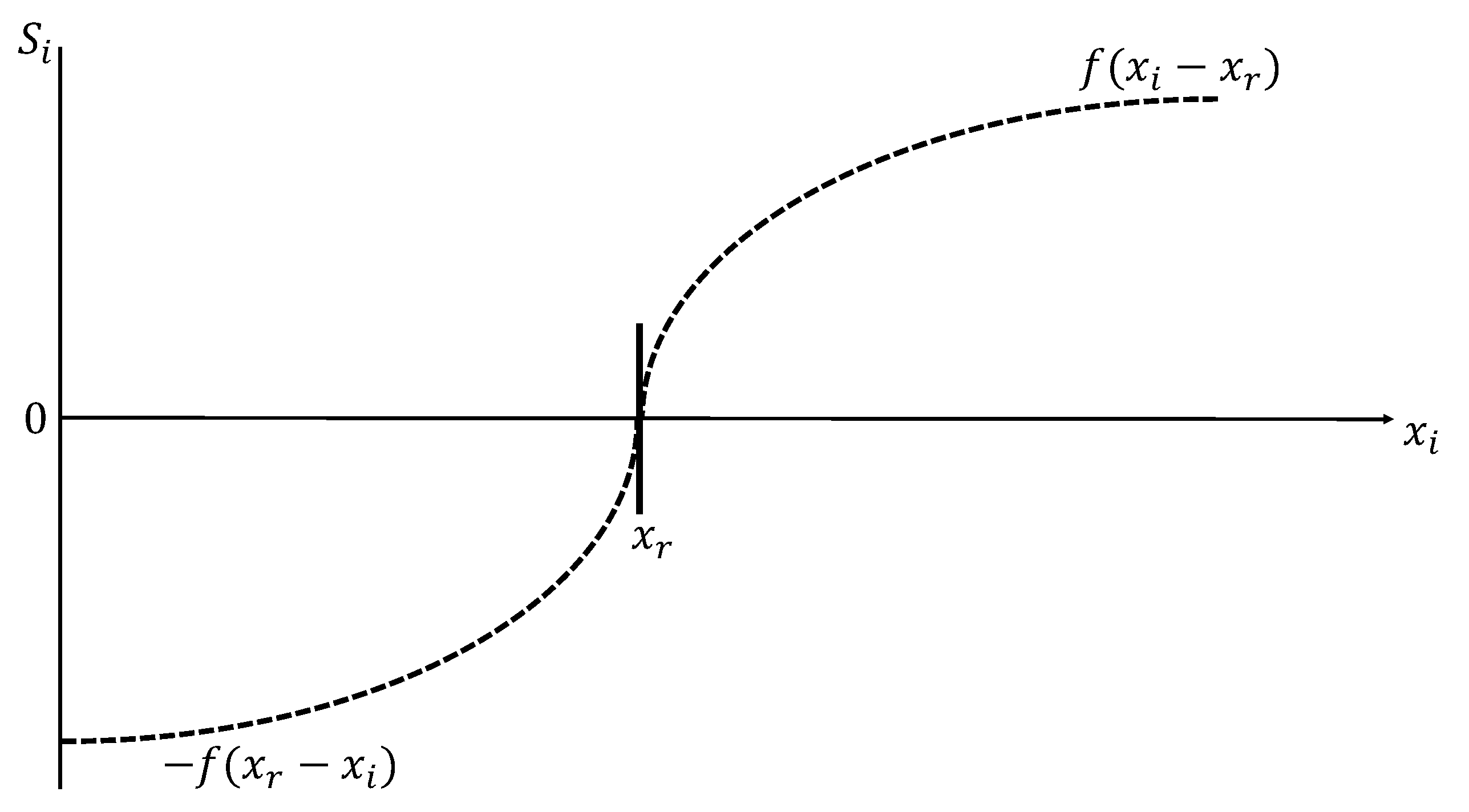
6.
If instead f were convex, then the social esteem would have grown unboundedly and no finite equilibrium would have existed.
7.
The functional form for f and how it is normalized based on x r are akin to the reference-point effect of Kahneman and Tversky [32]. This reference-point effect also differentiates our model from that of Clark and Oswald (1998), who assume the same curvature on both sides of the reference point. Thus, our model relates to theirs like Prospect Theory relates to vNM’s Expected Utility Theory.
8.
Note that f Δ x * Δ x * is the average slope of the function f Δ x in the range 0 , Δ x * , in which its slope decreases from f 0 > k to f Δ x * = k . Thus, the intersection of the two conditions f 0 > k and f Δ x * Δ x * 2 k is non empty. For example, if f Δ x is a concave power function (i.e., f Δ x = A Δ x β for some β < 1 ), restriction (iii) f Δ x * Δ x * < 2 k translates to β 1 / 2 .
9.
Hence, restriction (iii) is required for the existence of a pure NE.
10.
If the game was extended to n players the nature of the result would be similar: the bottom contributor would contribute zero and the remaining n-1 players would contribute Δ x * .
11.
In the special case of x r = x ^ there exists another pure-strategy NE in which x i = 0 for the bottom contributor while x i = x ^ for the two others. In this equilibrium all players are indifferent between choosing x i = 0 and x i = x ^ .
12.
To see this graphically, imagine moving the reference point rightward in Figure 1 and how this changes the negative esteem of contributing zero.
13.
If the game was extended to n players, the nature of the result would be similar: there would exist multiple equilibria which differ in the level of the reference point but where all players contribute the same.
14.
Another potential deviation is that the median could surpass the top contributor. This would make the current top contributor the “new median” implying that the most profitable deviation is to surpass the “new median” by Δ x * . As is clear from the proof, the relative costs and benefits of this potential deviation are independent of the reference point and it is ruled out by the restrictions we have imposed on f to fulfill f Δ x * Δ x * < 2 k . If this condition does not hold there would exist no equilibrium in pure strategies.
15.
If the game was extended to an odd number of n players the nature of the result would be similar. There would exist multiple equilibria differing in the reference point contribution, where in each equilibrium the bottom n + 1 2 players would contribute the same as the median reference while the remaining n 1 2 players would contribute x r + Δ x * .
16.
Δ x * < x ^ (by Lemma A2 in Appendix A) f Δ x * < f x ^ = k x ^ = 1 a / 3 x ^ , implying that the welfare difference given by (4) is greater than a 1 3 x ^ Δ x * 1 a / 3 x ^ > 2 a 1 x ^ 1 a / 3 x ^ = 7 3 a 3 x ^ .
17.
Since in this comparison x r = 0 in all methods, also the welfare is higher under the bottom-contributor comparison method.
Figure 1. Social esteem function.
Games 09 00097 g001

