
Asymptotic Solutions of Steady Lamellar Eutectic Growth in Directional Solidification for Small Tangent Values of the Contact Angles
National-Local Joint Engineering Laboratory for Technology of Advanced Metallic Solidification Forming and Equipment, School of Materials Science and Engineering, Kunming University of Science and Technology, Kunming 650093, China
*
Author to whom correspondence should be addressed.
Crystals 2024, 14(1), 93; https://doi.org/10.3390/cryst14010093
Submission received: 3 December 2023
/
Revised: 30 December 2023
/
Accepted: 16 January 2024
/
Published: 19 January 2024
Abstract
:A system of steady lamellar eutectic growth in directional solidification is considered with the case of small tangent values of the contact angles. The mathematical model is given in the non-dimensional rectangular coordinate system and the uniformly valid asymptotic solutions are obtained based on the method of the asymptotic expansions. The necessary condition for existing asymptotic solutions was obtained. The results indicate that the curvature undercooling and the solute undercooling determined the patterns of the solid–liquid interface. The dimensional average undercooling presents a relationship with eutectic spacing and pulling velocity. It can be seen that the dimensional average undercooling in front of both phases is not equal, and the total average undercooling as a function of the lamellar eutectic spacing exhibits a minimum. The minimum undercooling spacing decreases with an increase in the pulling velocity, which is in good agreement with Jackson and Hunt’s results.
1. Introduction
For the fixed solidification velocity and the thermal gradient, the directional solidification of a eutectic binary alloy produces two coupled crystal phases, and . The growth of the two coupled phases from the bulk melt is essentially controlled by the solute diffusion [1]. The eutectic microstructures in directional solidification have been theoretically investigated for decades. Faivre et al. [2,3,4,5] found that there are several stable patterns in their experimental study of CBr4-C2Cl6 lamellar eutectic growth. They showed that the stationary, relfection-symmetric, spatially periodic, and 2D patterns are stable within a finite range of the eutectic spacing for the fixed pulling velocity and the solute concentration. In their work, they found six different types of low-symmetry extended growth patterns and five new types of oscillatory or tilted states. Bottin-Rousseau et al. [6] investigated the directional solidification dynamics of Al-Al2Cu alloys and established a link between the growth of locked, tilted–lamellar patterns and the crystal orientation. Bottin-Rousseau et al. [7] observed a large-scale coexistence between rod and lamellar eutectic growth patterns during the directional solidification of succinonitrile–camphor eutectic alloys. Serefoglu et al. [8] studied an in situ experiment of the lamellar-to-rod transition during the directional solidification of succinonitrile–camphor eutectic alloys. The evolution of eutectic solid–liquid interfacial morphology and its growth stability have become important topics of concern for researchers. Among these theories, many results have been presented using numerical calculation methods [9,10,11,12,13,14,15,16,17,18,19,20]. Liu et al. [9] showed that the steady growth of lamellar eutectics had a limited range of spacings by using the boundary element method and an iterative technique. The minimum spacing corresponds to the result predicted by Jackson and Hunt [21], but the maximum spacings are less than the Jackson–Hunt result. Folch et al. [11] developed a phase-field model with which quantitative simulations of low-speed eutectic solidification were presented under typical experimental conditions. Feng et al. [12] and Zhang et al. [13] considered the influence of fluid flow on the lamellar eutectic growth by using phase field modeling, respectively. Pusztai et al. [15] studied the melting of 2D lamellar and 3D rod eutectic growth by using multi-phase field simulations, and found that melting occurs with a nearly flat interface if the average composition of the initial solid is equal to the eutectic composition. Tu et al. [16] studied the lamellar growth with solid–solid boundary anisotropy in directional solidification calculated using the phase-field method. Akamatsu et al. [17] presented two-dimensional numerical simulations of tilted lamellar growth in directional solidification of nonfaceted binary eutectic alloys by using a dynamic boundary-integral method. Ogawa et al. [18] developed a multiphase cellular automaton model for eutectic solidification. They observed the rod splitting when the rod spacing was large. Yang et al. [19] studied the effect of convection on 3D eutectic growth by employing a multi-phase field lattice–Boltzmann method. Seiz et al. [20] reproduced dendritic, eutectic, as well as dendritic–eutectic growth by using a phase-field model.
In addition to the important results based on numerical simulations above, many analytical theories of eutectic growth are presented [21,22,23,24,25,26,27,28,29,30,31,32]. Jackson and Hunt [21] developed a diffusion theory for the growth of eutectics and gave the analytical solutions of the steady eutectic system when they supposed the solidifying interfaces were planar and isothermal. If the average undercoolings of the -liquid and the -liquid interfaces were equal, they considered that there existed a minimum of the average undercooling for some critical eutectic spacing. Datye et al. [22] performed a stability analysis following Jackson–Hunt’s work. They found that, for all values of solute composition or temperature gradient, there was a long wavelength instability at lamellar spacing less than a critical value, as predicted by Jackson and Hunt [21]. Brattkus et al. [23] took into account the system of the lamellar eutectic under large thermal gradients (the morphological number ) and obtained the solute concentration solutions by using the integral method assuming planar solid–liquid interfaces. Chen and Davis [24] derived the steady solutions based on the method of multiple-scale expansions with small contact angles as the morphological number, and the surface energy number, , where is the order of interfacial amplitude relative to the lamellar spacing. is the small Peclet number. In their work, they relaxed the Jackson–Hunt assumption, and also predicted a critical lamellar spacing. Their results with a large morphological number agree with those given by Jackson and Hunt. Recently, Xu et al. [26,27] considered the system of eutectic growth for contact angles of a normal order and gave steady solutions on the assumption that the partition coefficient is close to the unit and the parameter, . As the contact angles are of a normal order, there is a singularity at the triple point. They derived the global steady-state solutions using the multiple variables expansion method. The multiple-scale expansions method or the multiple variables expansion method is one of the asymptotic analysis methods that are effective for solving multi-scale engineering problems such as systems of eutectic growth. However, all the above obtained analytical solutions of eutectic growth are based on the assumption that the surface energy number or other dimensionless parameters (such as the morphological number, the partition coefficient minus one, etc.) have special orders. Recently, we presented the asymptotic solutions of a rod eutectic system with small tangent values of the contact angle and normal orders and studied the linear instability mechanism of rod eutectic growth [27,28,29,30,31].
In this paper, we will consider the lamellar eutectic system for small tangent values of the contact angle and generalize the solution given by Chen et al. [24]. We will give the necessary conditions for existence of the steady solutions using the asymptotic method. Finally, we will determine the liquid-solid interfacial shapes and discuss the effects of eutectic spacing on the average undercooling.
2. Mathematical Formulation
A binary alloy with an initial solute concentration near the eutectic concentration is solidified unidirectionally with a pulling velocity V and a temperature gradient G, and then produces a periodic arrangement of two solid phases ( and phases). We assume that the – interface is parallel to the direction of the pulling velocity and neglect the tilted patterns. The typical lamellar eutectic patterns are illustrated in Figure 1 and the lamellar eutectic system is described in a mathematical model as shown in Equations (1)–(6). We use half the eutectic spacing as the length scale and V as the velocity scale, in order to make the physical properties of the eutectic system dimensionless. The non-dimensional solute concentration is defined as . and are the solute concentrations of -phase and -phase at eutectic temperature , respectively. denotes the dimensional solute concentration. In the moving coordinate system , whose origin is located at the tip of the solid -phase shown in Figure 1, the diffusion equation, the interfacial conditions, and the boundary conditions are written as follows:
where and correspond to the first and second derivatives of the liquid–solid interface function with respect to x, respectively. The subscripts are the two solid phases.
For the sake of symmetry here, we only consider the system at interval along the lateral axis x. The constant is the volume fraction of the -phase in the solid and is also the abscissa of a triple point. Equation (1) describes the diffusion equation in the liquid phase and the diffusion in the solid phases is neglected because its diffusion coefficient is extremely small. The Peclet number is defined as
where denotes the solute diffusion coefficient in the liquid phase. Equation (2) is the Gibbs–Thomson condition accounting for the interaction among interface curvature, solute concentration and temperature at the solid–liquid interfaces. The unfixed constant indicates the position of the eutectic temperature . The nondirectional parameter , the morphological number and the surface energy number are denoted as
where denotes the liquidus slope of the phase diagram, is the latent heat per unit volume, is the interfacial tension among -liquid interface and is the miscibility gap. Here, are introduced. Equation (3) describes the solute conservation, where is the partition coefficient. Equation (5) is the local equilibrium condition at the triple points, and contact angle is determined by the Young’s law. Finally, Equation (6) is the far field condition, where is the dimensionless initial solute concentration in the liquid phase.
We will search for the asymptotic solutions of the above mathematical model. As Chen and Davis did [24], we assume that the Peclet number is small, . In other words, the lamellar spacing, is much smaller than the diffusion length , which is, indeed, consistent with the actual experimental results. We also assume the amplitude of the solid–liquid interface to be much smaller than the eutectic spacing, i.e., . Due to the existence of multiple scales (the lamellar spacing, the interfacial amplitude and the diffusion length) in the system of the lamellar eutectic growth, we still use the asymptotic expansion method and the matching method to solve the solutions of the mathematical model. As , we will divide the whole liquid region of the eutectic system into two regions because of the different length scales: the outer region, which is far away from the liquid–solid interface, and the inner region, which is close to the liquid–solid interface. We will derive the solutions in each region by using the asymptotic expansion method, and obtain the composite solutions by using the matching method. The solutions in each region will be derived using the asymptotic expansion method. Finally, all the asymptotic solutions will be matched in the intermediate region and the composite solution will be obtained.
3. Outer Solutions in the Region Far from the Liqiud–Solid Interface
The solute diffusion in the region far from the liquid–solid interface is not effected by liquid–solid interfacial morphology as , so the solute concentration function is independent of the variable x. Hence, the solid–liquid interface may be considered as a planar. In this region, we present the outer variable
The outer solutions of the solute concentration field are denoted as , which meet the following equation:
and the solute concentration , as . The asymptotic solutions of Equation (8) meeting the far field condition are as follows:
where constants, and the small parameter, , will be determined by matching the above outer solutions with the solute concentration solutions near the liquid–solid interface. Note that the outer solution is independent of the variable, x; thus, the above results of the lamellar eutectic system are consistent with those of the rod eutectic system [29,30].
4. Solutions in the Region Near the Liquid–Solid Interface
In the liquid phase region near the liquid–solid interface, we need to determine both the solute concentration and the interfacial shapes simultaneously. They are determined by the Gibbs–Thomson condition and the mass conservation condition. We now give the solution of the solute concentration and the solid–liquid interfacial function , based on Equations (1)–(4) and
For , we first solve from Equations (1), (3), (4) and (10), then obtain from Equations (2), (4) and (5) using the asymptotic expansion method. Hence, the interfacial order is determined by . We rewrite the Gibbs–Thomson condition as follows:
The left-hand three terms of Equation (11), respectively, correspond to the curvature, interface and solute undercoolings [21], namely,
where , , and . Note that the undetermined constant may be one or of a smaller order. Equation (12) indicates that , corresponding to the interfacial shape, is determined by the curvature undercooling and the solute undercooling .
If the curvature undercooling, the solute undercooling and the interface undercooling are of the same order, we can obtain the following relationships as ,
Chen-Davis [24] assumed that , , , . Obviously, this is one of the above equations, Equation (13). We can write
where the constant , and . Equation (14) is the necessary condition for the existence of the steady solutions using the asymptotic method.
As , and combining with the case of the small tangent values of the contact angles and the small interfacial amplitude, we have
Hence, combining with condition (5), we limit that . In other words, as , ,where .
For the first-order approximation, the solute concentration function and the interface function , meet the Laplace equation and boundary conditions as follows:
Here, and . We will first solve the concentration field by using Equation (16a) and conditions (10) and (16c); then, we will obtain the interface function from (16b) following Chen-Davis’s method.
As , the step function can be written as the Fourier cosine expansion form
whose Fourier coefficients are calculated as
Combining with Equation (17), the solute-concentration solution of Equation (16a) meeting the condition (16c) is derived as follows:
where is a fixed constant. By using the matching condition as and , or
One can fix the constant and the relationship or
This equation denotes the relationship of with . Note that, for a eutectic system, the initial concentration is mostly near the eutectic concentration, hence . But in our mathematical model of a eutectic system, the obtained solutions above also contain the case of , which was considered by Chen et al.
The interface function is easily obtained from Equation (16b):
where
5. Uniformly Valid Solutions
In previous sections, the solution in each region was derived by using the asymptotic expansions method for . But these solutions are not uniformly valid in the whole system of eutectic growth. Here, we can obtain the uniformly valid solutions based on the matching condition in the intermediate region. The composite solutions are the sum of the outer solutions and the inner solutions corrected by subtracting the part they have in common.
For , the composite solutions of the eutectic system are
Now, the steady asymptotic solutions of the lamellar eutectic growth have been obtained as and .
6. Average Undercooling of the Solid–Liquid Interface
In this section, we will study the effects of lamellar eutectic spacing on the interface undercooling . As , the interface undercooling corresponds to the Gibbs–Thomson condition. Combining with Equation (12), we can obtain the interface undercooling
From Equation (24), the average undercooling of the interface in front of -liquid phase is calculated,
and in front of -liquid phase,
where . As , . We can rewrite . Combining with Equations (25) and (26), the total average undercooling is written as follows:
or
The dimensional average undercooling is given as follows:
Combining with , we obtain a relationship between the dimensional undercooling and the lamellar eutectic spacing ,
7. Discussion
We have obtained the steady asymptotic solutions for the lamellar eutectic system for the case of and . Combining with the morphological number and the surface energy number , the condition can be written as . If the solute concentration solutions are given, Equation (11) has the exact same solution as . If the solutions of the solute concentration (18) are effective for the eutectic system, the interface solutions (21) can be applied to any case as . Hence, as , the steady interface solutions (23) are accepted for all the values of if the solute concentration solutions are valid for the eutectic growth system.
Figure 2 presents solid–liquid interfaces of eutectic growth. It can be seen that Figure 2 has a convex interface. The interface patterns (convex or concave) are mainly determined by the curvature undercooling and the solute undercooling. The curvature undercooling leads to a stable interface and the solute undercooling causes an unstable interface. If the interface undercooling is mainly determined by the solute undercooling, the liquid–solid interface will be concave. On the other hand, curvature undercooling will promote a convex interface. For the case of , , , the average undercooling is given in Figure 3. This figure shows that the curvature undercooling gradually increases as x changes from tips of solid phases to the triple point along the solid–liquid interface, while the solute undercooling has the opposite relationship. If the increase of the curvature undercooling exceeds the decrease of the solute undercooling, then it will lead to an interface undercooling increase, and finally to convex interface formation. It can also be seen that curvature undercooling is the main factor and that it leads to the convex interface shown in Figure 2.
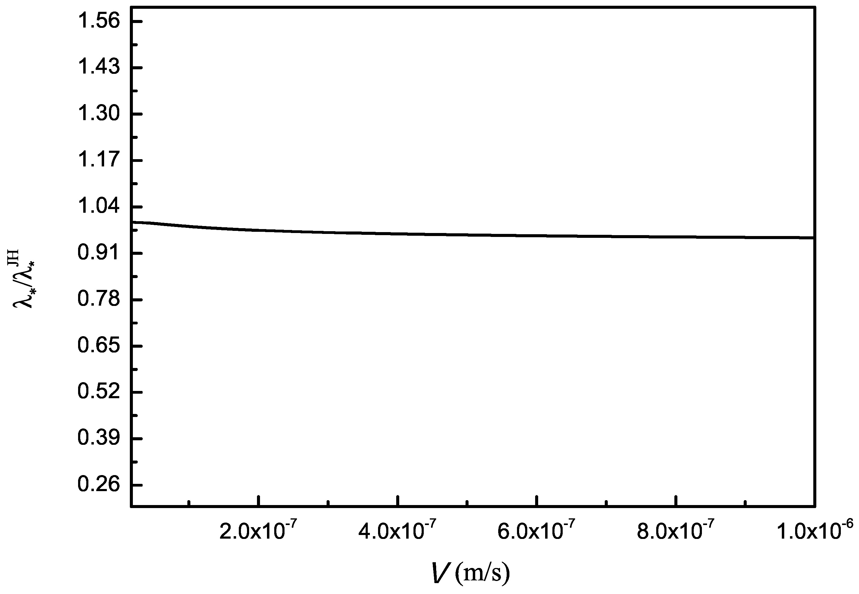
In the above section, we have already obtained the expression of solid–liquid interface undercooling and presented the relationship between the average undercooling and the lamellar eutectic spacing. Jakson and Hunt, in their work [21], assumed that the average undercoolings in front of both phases are equal in order to find the analytical solution of eutectic growth. Figure 4 shows the relationships of the average undercoolings of the -phase interface and the -phase interface with the lamellar eutectic spacing with . In our results, we relax this assumption and it is seen that the average undercooling of the -phase interface is not equal to the and -phase interface. Figure 5 shows that the relationship between the total average undercooling and the lamellar eutectic spacing for: . This figure shows that there exists a minimum for the total average undercooling, which is in agreement with the Jackson and Hunt’s [21] results. The eutectic spacing corresponding to the minimum of the average undercooling, , is called the minimum undercooling spacing. We present the effect of pulling velocity on the minimum undercooling spacing and compare this with Jackson and Hunt’s results shown in Figure 6. The minimum of the undercooling spacing decreases with an increase in the pulling velocity. It can also be seen that our result is in agreement with Jackson and Hunt’s result. Figure 7 shows that as a function of V. From this figure, we can seen that changes from 0.99 to 0.95 when the pulling velocity changes from to .
8. Conclusions
The steady system of lamellar eutectic growth under directional growth was considered, in which the Young’s law is met at the triple points for a small-order the tangent of the contact angles. Based on work by Chen et al. [24], we obtained the generalized solution and presented the necessary conditions of a uniformly valid solution of eutectic growth. Due to the different scales in different regions, solutions in every region are obtained using asymptotic expansion methods. The uniformly valid solutions in the whole liquid region of the system are derived by using the matching method. We have presented solid–liquid interface shapes and the average undercoolings in front of both phases. The curvature undercooling and the solute undercooling determine the liquid–solid interface shapes. The curvature undercooling leads to the stable interface and the solute undercooling is to cause the unstable interface. The total average undercooling as a function of the eutectic spacing exhibits a minimum. The minimum undercooling spacing decreases with an increase in the pulling velocity, which is in good agreement with Jackson and Hunt’s result. If we ignore the principle of the minimum undercooling, we actually have obtained many solutions with free eutectic spacing. Next, we will investigate the stability of eutectic growth following our steady asymptotic solutions. A quantitative prediction of the stable morphology of eutectic growth will be the focus of our future research.
Author Contributions
Methodology, X.L.; formal analysis, J.X.; writing—original draft preparation, J.X.; writing—review and editing, X.L.; project administration, X.L.; funding acquisition, X.L. All authors have read and agreed to the published version of the manuscript.
Funding
This research was funded by the National Natural Science Foundation of China (No. 51961018).
Data Availability Statement
Data are contained within the article.
Conflicts of Interest
The authors declare no conflicts of interest.
References
- Glicksman, M.E. Principles of Soldification; Springer: London, UK, 2011; pp. 398–424. [Google Scholar]
- Faivre, G. Morphological instabilities of lamellar eutectic growth fronts: A survey of recent experimental and numerical results. J. Cryst. Growth 1996, 166, 29–39. [Google Scholar] [CrossRef]
- Ginibre, M.; Akamatsu, S.; Faivre, G. Experimental determination of the stability diagram of a lamellar eutectic growth front. Phys. Rev. E 1997, 56, 780–796. [Google Scholar] [CrossRef]
- Mergy, J.; Faivre, G.; Guthmann, C.C.; Mellet, R. Quantitative determination of the physical parameters relevant to the thin-film directional solidification of the CBr4-C2Cl6 eutectic alloy. J. Cryst. Growth 1981, 134, 353–368. [Google Scholar] [CrossRef]
- Akamatsu, S.; Plapp, S.; Faivre, G.; Karma, A. Pattern stability and trijunction motion in eutectic solidification. Phys. Rev. E 2002, 66, 030501. [Google Scholar] [CrossRef] [PubMed]
- Bottin-Rousseau, S.; Medjkoune, M.; Senninger, O.; Carroz, L.; Soucek, R.; Hecht, U.; Akamatus, S. Loked-lamellar eutectic growth in thin Al-Al2Cu samples: In situ directional solidification and crystal orientation analysis. J. Cryst. Growth 2021, 570, 126203. [Google Scholar] [CrossRef]
- Bottin-Rousseau, S.; Witusiewicz, V.; Hecht, U.; Fernandez, J.; Laveron-Simavilla, A.; Akamatus, S. Coexistence of rod-like and lamellar eutectic growth patterns. Scr. Mater. 2022, 207, 11314. [Google Scholar] [CrossRef]
- Serefoglu, M.; Bottin-Rousseau, S.; Akamatsu, S. Lamella-rod pattern transition and confinement effects during eutectic growth. Acta Mater. 2023, 242, 118425. [Google Scholar] [CrossRef]
- Liu, J.; Elliott, R. A numerical model for eutectic spacing selection in the CBr4C2cl6 eutectic system. J. Cryst. Growth 1995, 148, 406–414. [Google Scholar] [CrossRef]
- Pusztai, T.; Tatkai, L.; Szallas, A.; Granasy, L. Spiraling eutectic dendrites. Phys. Rev. E 2013, 87, 032401. [Google Scholar] [CrossRef]
- Folch, R.; Plapp, M. Quantitative phase-field modeling of two-phase growth. Phys. Rev. E 2005, 72, 011602. [Google Scholar] [CrossRef]
- Feng, L.; Feng, X.; Lu, Y.; Zhu, C.; Jia, B. Phase field modeling of lamellar eutectic growth under the influence of fluid flow. Comp. Mater. Sci. 2017, 137, 171–178. [Google Scholar] [CrossRef]
- Zhang, A.; Guo, Z.; Xiong, S.M. Quantitative phase-field lattice-Boltzmann study of lamellar eutectic growth under natural convection. Phys. Rev. E 2018, 97, 053302. [Google Scholar] [CrossRef] [PubMed]
- Lei, W.; Cao, Y.; Xin, L.; Kun, C.; Huang, W. Globular to lamellar transition during anomalous eutectic growth. Model. Simul. Mater. Sci. Eng. 2020, 28, 065014. [Google Scholar] [CrossRef]
- Pusztai, T.; Ratkai, L.; Horvath, L.; Granasy, L. Phase-field modeling of directional melting lamellar and rod eutectic structures. Acta Mater. 2022, 227, 117678. [Google Scholar] [CrossRef]
- Tu, Z.; Zhou, J.; Tong, L.; Guo, Z. A phase-field study of lamellar eutectic growth with solid-solid boundary anisotropy. J. Cryst. Growth 2019, 532, 125439. [Google Scholar] [CrossRef]
- Akamatsu, S.; Bottin-Rousseau, S. Numerical Simulations of Locked Lamellar Eutectic Growth Patterns. Metall. Mater. Trans. A 2021, 52, 4533–4545. [Google Scholar] [CrossRef]
- Ogawa, J.; Natsume, Y. Cellular automaton model for predicting the three-dimensional eutectic structure of binary alloys. Comp. Mater. Sci. 2021, 195, 110497. [Google Scholar] [CrossRef]
- Yang, Q.; Zhang, A.; Jiang, B.; Gao, L.; Guo, Z.; Song, J.; Xiong, S.; Pan, F. Numerical investigation of eutectic growth dynamics under convection by 3D phase-field method. Comp. Math. App. 2022, 114, 83–94. [Google Scholar] [CrossRef]
- Seiz, M.; Kellner, M.; Nestler, B. Simulation of dendritic-eutectic growth with the phase-field method. Acta Mater. 2023, 254, 118965. [Google Scholar] [CrossRef]
- Jackson, K.A.; Hunt, J.D. Lamellar and rod eutectic growth. Trans. Metall. Soc. AIME 1966, 236, 1129. [Google Scholar]
- Datye, V.; Langer, J.S. Stability of thin eutectic growth. Phys. Rev. B 1981, 24, 4155–4169. [Google Scholar] [CrossRef]
- Brattkus, K.; Caroli, B.; Caroli, C.; Roulet, B. Lamellar eutectic growth at large thermal-gradient. 1. stationary pattern. J. Phys. Fr. 1990, 51, 1847–1864. [Google Scholar] [CrossRef]
- Chen, Y.J.; Davis, S.H. Instability of triple junctions in lamellar eutectic growth. Acta Mater. 2001, 49, 1363–1372. [Google Scholar] [CrossRef]
- Akamatsu, S.; Bottin-Rousseau, S.; Serefoglu, M.; Faivre, G. A theory of thin lamellar eutectic growth with anisotropic interphase boundaries. Acta Mater. 2012, 60, 3199–3205. [Google Scholar] [CrossRef]
- Li, X.M.; Li, W.Q.; Jin, Q.L.; Zhou, R. A steady solution of the gasar eutectic growth in directional solidification. Chin. Phys. B 2022, 80, 078101. [Google Scholar] [CrossRef]
- Xu, J.J.; Li, X.M. Global steady state solutions for lamellar eutectic growth in directional solidification. J. Cryst. Growth 2014, 401, 93–98. [Google Scholar] [CrossRef]
- Xu, J.J.; Chen, Y.Q. Steady spatially-periodic eutectic growth with the effect of triple point in directional solidification. Acta Mater. 2014, 80, 220. [Google Scholar] [CrossRef]
- Li, X.M.; Xu, F. Uniformly valid asymptotic solutions of rod eutectic growth in directional solidification for contact angles being the normal order. J. Cryst. Growth 2017, 468, 945–949. [Google Scholar] [CrossRef]
- Li, X.M.; Chen, X.K.; Xu, F. Uniformly valid asymptotic solutions of rod eutectic growth in directional solidification for liquid-solid interface slopes of small order. J. Cryst. Growth 2019, 507, 453–458. [Google Scholar] [CrossRef]
- Gan, Y.L.; Li, X.M. Global instability of rod eutectic growth in directional solidification. Crystals 2023, 13, 548. [Google Scholar] [CrossRef]
- Tu, Z.; Zhou, J.; Zhang, Y.; Li, W.; Yu, W. An analytic theory for the symmetry breaking of growth-front in lamellar eutectic growth influenced by solid-solid anisotropy. J. Cryst. Growth 2020, 549, 125851. [Google Scholar] [CrossRef]
Figure 1.
Sketch of lamellar eutectic growth in reference frame .
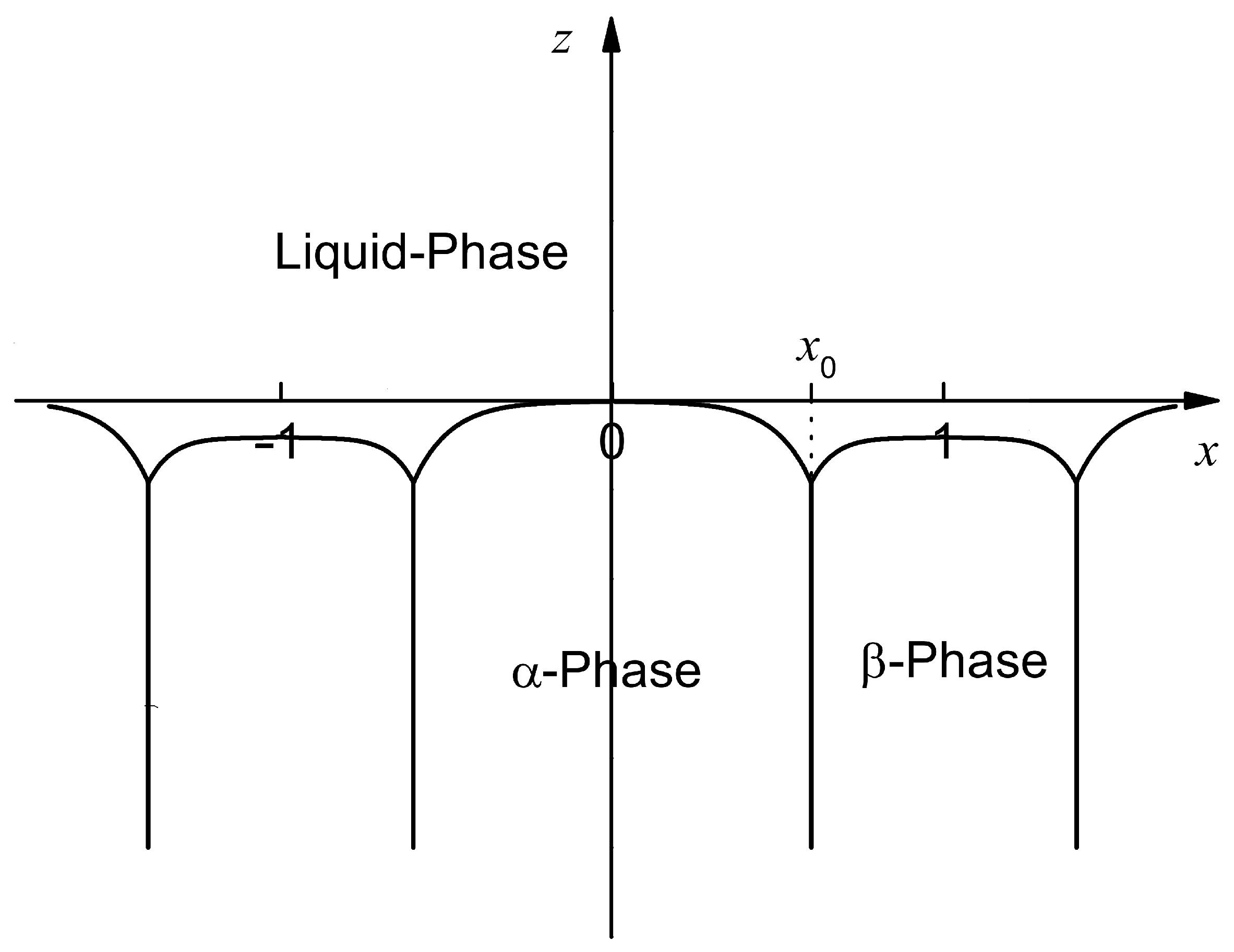
Figure 2.
Solid–liquid interfacial function h with x for the case of , .

Figure 3.
Curvature composite and thermal undercoolings with x for the case of ,

Figure 4.
The relationship between the dimensional average undercooling of the s-phase interface and the lamellar eutectic spacing for .
Figure 4.
The relationship between the dimensional average undercooling of the s-phase interface and the lamellar eutectic spacing for .

Figure 5.
The relationship between the dimensional average undercooling of the solid–liquid interface, and the lamellar eutectic spacing for .
Figure 5.
The relationship between the dimensional average undercooling of the solid–liquid interface, and the lamellar eutectic spacing for .
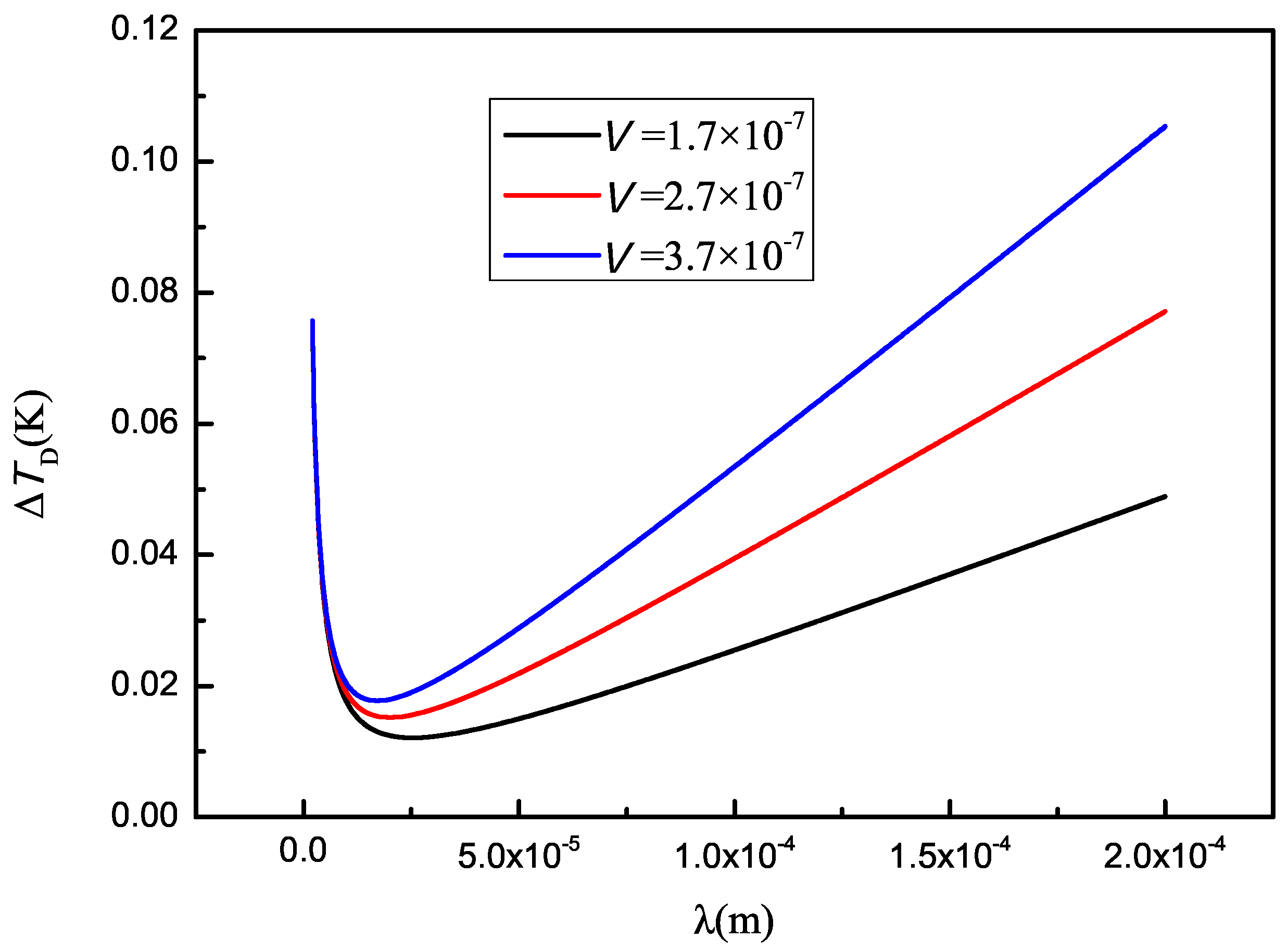
Figure 6.
The relationship between the minimum undercooling spacing, , and the pulling velocity, V.
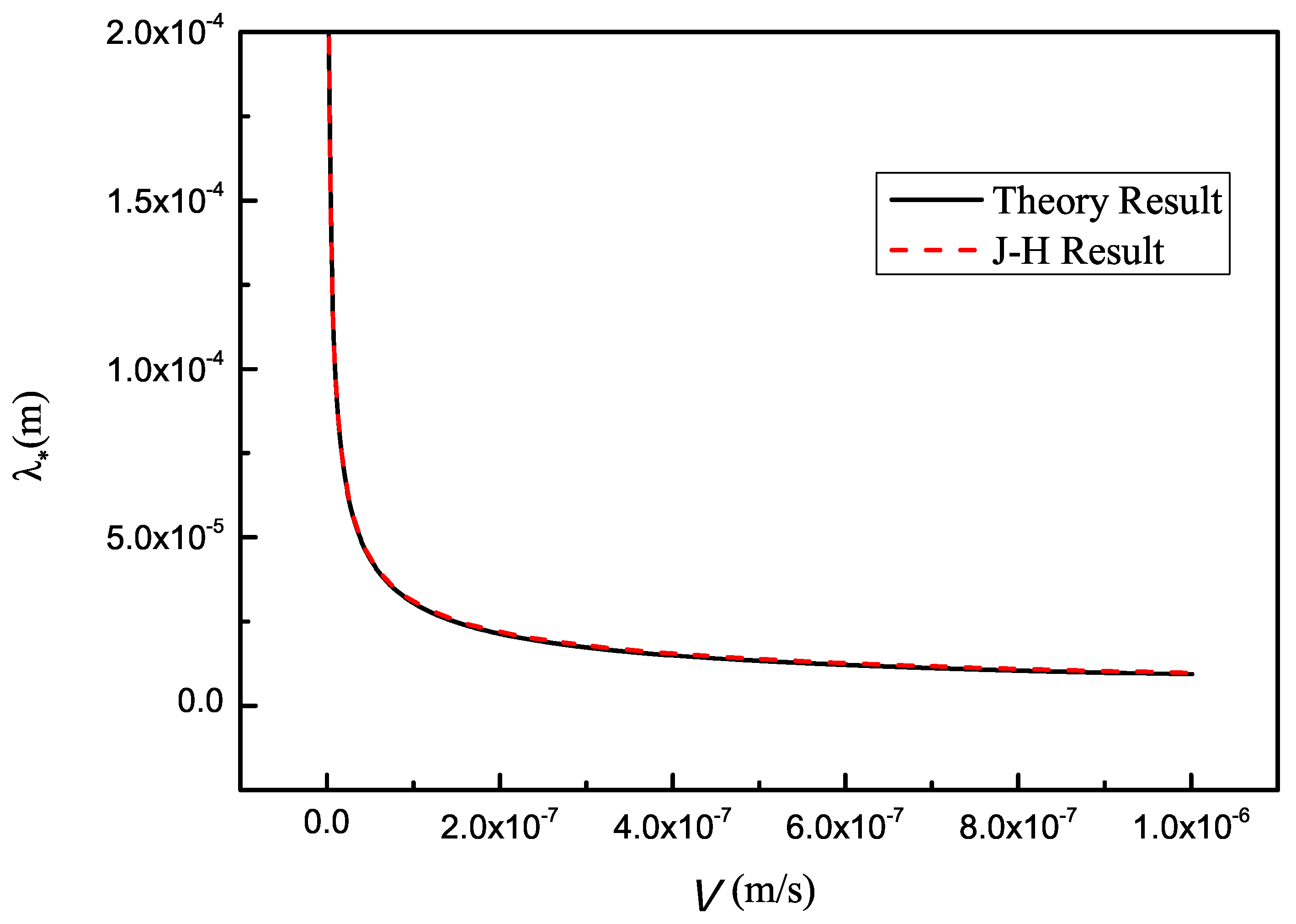
Figure 7.
as a function of the pulling velocity, V.
Disclaimer/Publisher’s Note: The statements, opinions and data contained in all publications are solely those of the individual author(s) and contributor(s) and not of MDPI and/or the editor(s). MDPI and/or the editor(s) disclaim responsibility for any injury to people or property resulting from any ideas, methods, instructions or products referred to in the content. |
© 2024 by the authors. Licensee MDPI, Basel, Switzerland. This article is an open access article distributed under the terms and conditions of the Creative Commons Attribution (CC BY) license (https://creativecommons.org/licenses/by/4.0/).
Share and Cite
MDPI and ACS Style
Xiao, J.; Li, X. Asymptotic Solutions of Steady Lamellar Eutectic Growth in Directional Solidification for Small Tangent Values of the Contact Angles. Crystals 2024, 14, 93. https://doi.org/10.3390/cryst14010093
AMA Style
Xiao J, Li X. Asymptotic Solutions of Steady Lamellar Eutectic Growth in Directional Solidification for Small Tangent Values of the Contact Angles. Crystals. 2024; 14(1):93. https://doi.org/10.3390/cryst14010093
Chicago/Turabian StyleXiao, Jing, and Xiangming Li. 2024. "Asymptotic Solutions of Steady Lamellar Eutectic Growth in Directional Solidification for Small Tangent Values of the Contact Angles" Crystals 14, no. 1: 93. https://doi.org/10.3390/cryst14010093
Note that from the first issue of 2016, this journal uses article numbers instead of page numbers. See further details here.