A Numerical Method for Flexural Vibration Band Gaps in A Phononic Crystal Beam with Locally Resonant Oscillators


1
Ocean College, Zhejiang University, Zhoushan 316021, China
2
Department of Naval Architecture, Ocean and Marine Engineering, University of Strathclyde, Glasgow G1 5AE, UK
*
Authors to whom correspondence should be addressed.
Crystals 2019, 9(6), 293; https://doi.org/10.3390/cryst9060293
Submission received: 27 April 2019
/
Revised: 2 June 2019
/
Accepted: 3 June 2019
/
Published: 5 June 2019
(This article belongs to the Special Issue Sonic and Photonic Crystals)
Abstract
:The differential quadrature method has been developed to calculate the elastic band gaps from the Bragg reflection mechanism in periodic structures efficiently and accurately. However, there have been no reports that this method has been successfully used to calculate the band gaps of locally resonant structures. This is because, in the process of using this method to calculate the band gaps of locally resonant structures, the non-linear term of frequency exists in the matrix equation, which makes it impossible to solve the dispersion relationship by using the conventional matrix-partitioning method. Hence, an accurate and efficient numerical method is proposed to calculate the flexural band gap of a locally resonant beam, with the aim of improving the calculation accuracy and computational efficiency. The proposed method is based on the differential quadrature method, an unconventional matrix-partitioning method, and a variable substitution method. A convergence study and validation indicate that the method has a fast convergence rate and good accuracy. In addition, compared with the plane wave expansion method and the finite element method, the present method demonstrates high accuracy and computational efficiency. Moreover, the parametric analysis shows that the width of the 1st band gap can be widened by increasing the mass ratio or the stiffness ratio or decreasing the lattice constant. One can decrease the lower edge of the 1st band gap by increasing the mass ratio or decreasing the stiffness ratio. The band gap frequency range calculated by the Timoshenko beam theory is lower than that calculated by the Euler-Bernoulli beam theory. The research results in this paper may provide a reference for the vibration reduction of beams in mechanical or civil engineering fields.
1. Introduction
Phononic crystals (PCs) are periodic composites or structures which modify the band structure in some way. The band gap is a frequency range in which the propagation of elastic waves in phononic crystal structures is suppressed. By adjusting the parameters of the artificial periodic structure, the position and width of the band gap and its ability to suppress wave propagation can be artificially regulated. In engineering practice, structures can be designed as phononic crystals, and then the band gap characteristics can be used in vibration and noise reduction.
There are two formation mechanisms of the elastic band gap in PCs: one is the Bragg scattering mechanism [1,2,3,4,5,6,7,8,9,10,11,12,13,14,15,16,17,18], and the other is the locally resonant mechanism. The wave length corresponding to the elastic band gap formed by Bragg scattering is generally equal to the lattice size or lattice constant, which restricts its application in engineering practice. In 1999, Liu et al. [19] proposed the locally resonant mechanism of the elastic band gap. It was found that the corresponding wave length of this locally resonant phononic crystal is far larger than the lattice size, which breaks through the limitation of the Bragg scattering mechanism and opens up a wide potential for application in low-frequency wave band. Since then, investigations on the locally resonant mechanism of phononic crystals have been carried out continuously [20,21,22,23].
The study of the band gap mechanism of PCs depends on the solving methods of elastic wave band gaps. At present, computational methods of vibration band gaps mainly include the transfer-matrix method (TM), multiple-scattering theory (MST), finite difference time-domain method (FDTD), lumped-mass method (LM), plane wave expansion method (PWE), differential quadrature method (DQM), finite element method (FEM), extended plane wave expansion method (EPWE) [24], wave finite element method [25], and boundary element method (BE) [26]. The transfer-matrix method [27,28] is widely applied to calculate the band gap characteristics of 1-D PCs. Although the analytical solution can be obtained quickly, it is not suitable for the study of the vibration dispersion relations of 2-D and 3-D periodic structures, since the transfer matrix can usually only be transmitted in one direction. The PWE method [29,30] is the most basic and common method to calculate the band gap characteristics of phononic crystals. It can be used to solve the elastic band gap of all-dimensional PCs. However, when the material parameters vary greatly, or the filling rate is too high or too low, it is difficult to achieve convergence [31]. It is worth mentioning that in order to overcome the limitation of the convergence of PWE, the improved plane wave expansion (IPWE) method [26] is proposed. The FDTD method [32,33] can calculate the transmission, reflection, and energy band characteristics of infinite structures. However, the computational amount is large, and the large elastic constant difference may lead to numerical instability and divergence. The multiple scattering theory [34,35] can not only calculate the dispersion curves of periodic structures, but also disordered structures. It has fast convergence and high accuracy and is easy to deal with the problem of elastic mismatch, but only some kinds of scatterers with regular shape can be dealt with. At present, only phononic crystals composed of cylindrical (two-dimensional) and spherical (three-dimensional) scatterers can be calculated. The lumped mass method [36,37] converges fast, but there are some difficulties in dealing with multi-field coupling problems. The FEM method [38,39,40] is a commonly used method in engineering with good applicability, wide application range, and good convergence. There are various kinds of mature commercial software, such as Comsol, ANSYS, etc., which facilitate the modeling and analysis of complex periodic structures. The finite element method can be used to accurately calculate the band gap characteristics of PCs of various dimensions and various shapes of scatterers.
The differential quadrature method can approximate the value of each derivative of the function at the node with the weighted sum of the function values at all nodes in the domain and transforms the problem of the continuous system into a discrete problem. It has strong convergence and high precision. To the authors’ knowledge, the DQM was only applied to solve the elastic wave band gap of a beam or plate structure with the Bragg scattering mechanism [8,9]. However, the Bloch boundary conditions for locally resonant structures lead to nonlinear fundamental equations when using DQM, which causes difficulties in solving. Hence, numerical solutions of band gaps in LR structures based on DQM have not been reported up to now.
In this work, through applying an unconventional matrix-partitioning method and a variable substitution method, we transform the problem of solving the dispersion relation into a quadratic eigenvalue problem and propose a numerical method based on the differential quadrature method to calculate the bending vibration band gap of locally resonant beams. The purpose is to improve calculation accuracy and computational efficiency. Moreover, a parametric study is undertaken to investigate the effects of shear deformation and rotary inertia, the lumped mass, the spring stiffness coefficient, and the lattice size on the 1st band gap. Some major novelties of the contribution are pointed out as follows:
- (1)
- Based on the differential quadrature method, we propose a numerical method for calculating the flexural vibration band gaps of a locally resonant beam. In this paper, the differential quadrature method is applied to calculate the band gaps of locally resonant structures for the first time.
- (2)
- By using an unconventional matrix-partitioning method and a variable substitution method, we can transform the problem of solving the dispersion relation into a standard quadratic eigenvalue problem, and the problem of the non-linear term after using the DQM method can be solved easily.
- (3)
- Compared with the plane wave expansion method and the finite element method, the high accuracy and computational efficiency of the present method are demonstrated.
- (4)
- The proposed method has high precision and a rapid speed of convergence.
2. Method
2.1. Differential Quadrature Method
The basic idea of the differential quadrature method is to use the sum of the weighted values at all discrete points in the computational domain to approximate the unknown function values and their derivatives at any discrete points, so that the continuous system can be transformed into a discrete system for solving as follows.
where is the total number of discrete points in the calculation domain; ; ; are the Lagrange interpolation polynomials, and is the weight coefficient of the rth derivative defined by [41]:
where = 1, 2, …, Nx−1; i,j = 1, 2, …, Nx, (i ≠ j); and are defined as:
In order to obtain higher accuracy and faster convergence, the non-uniform mesh partition (Gauss-Lobatto-Chebyshev pattern) [42] is adopted in this paper. The coordinates of discrete points are as follows:
2.2. Unconventional Matrix-Partitioning Method & Variable Substitution Method
In the process of using the DQM method to calculate the band gaps of a locally resonant structure, a non-linear term of frequency exists in the matrix equation, which makes it impossible to solve the dispersion relationship by using the conventional matrix-partitioning method. Hence, we propose an unconventional matrix-partitioning method and a variable substitution method to calculate the flexural band gap of a locally resonant beam. The idea is to separate the nonlinear term from the matrix by unconventional matrix partitioning and variable substitution, and then transform the matrix equation into a quadratic eigenvalue problem. The proposed method is applicable to both the Euler–Bernoulli beam model and the Timoshenko beam model. The detailed application process is shown in Section 3.2. The following is a concise and general formulation of the proposed method.
where U is a vector of independent variables. Subscripts “q”, “b”, and “d” refer to the shear boundary condition, other boundary conditions, and the domain, respectively. Kqq(ω) is a scalar with the non-linear term. By variable substitutions and matrix operations, Equation (7) can be transformed into a quadratic eigenvalue problem.
For any given wave vector k in the first Brillouin zone, rz can be obtained by calculating the eigenvalue of matrix Hf. One can get the circular frequency ω due to Equation (10), thus the dispersion relation and bending vibration band gaps can be plotted.
3. Locally Resonant (LR) Beam Models and Solutions
Figure 1 shows the configuration of a straight elastic metamaterial beam with periodical locally resonant (LR) oscillator structures. Harmonic locally resonant oscillators are periodically connected along the x-axis to the infinite Euler beam. Each oscillator is formed by a lumped mass mz and a spring with stiffness kz, taking the distance between two adjacent LR oscillators as lattice size a. By extending the Euler-Bernoulli beam theory and the Timoshenko beam theory, one can obtain the theoretical model of the LR beam. Since the structure has infinite periodicity, we can apply the Floquet-Bloch theorem to simplify the whole model into a unit cell.
3.1. Euler–Bernoulli Model & Solution Procedures
When the length of each beam unit cell is much larger than its height and width, the Euler-Bernoulli approximation is satisfied, thus the influences of shear force and rotary inertia can be ignored. The governing equation for the bending vibration of the nth cell is shown below [43]:
where is the density; is Young’s modulus; is the cross-section area; is the area moment of inertia with respect to the axis perpendicular to the beam axis, and is the lateral displacement at . By assuming , where is the vibration amplitude of the beam at , and is the circular frequency, Equation (11) can be rewritten as follows:
For the (n + 1)th locally resonant oscillator, consider the balance of forces in the y-axis direction, we can get:
where is the interaction force between the beam and the oscillator at node , is the displacement of the lumped mass of the (n + 1)th oscillator, and the vibration amplitude of the (n + 1)th oscillator is denoted by the absolute value of .
According to Hooke's law, can be expressed as follows:
Substituting Equation (14) into Equation (13), one can get:
Ignoring the stress concentration between two adjacent units, the following boundary conditions can be listed according to the continuity of displacement, angle of rotation, bending moment, and shear force at the node .
According to the Floquet-Bloch theorem [44], Equations (16)–(19) can be rewritten as follows:
where is the Bloch wave vector, also known as the wave number.
To facilitate the application of DQM conveniently, the computational domain of each cell needs to be converted to a standardized computational domain [[−1,1] by the reversible transformation below:
where is the number of the cell; represents the coordinates of the left side of the nth beam unit; is equal to , and is the local coordinate in the normalized computational domain.
Substituting Equation (24) into Equation (12) and Equations (20)–(23), the governing equation and boundary conditions in the normalized computational domain can be obtained.
Substituting Equations (1)–(6) into Equations (25)–(29), the boundary conditions and governing equations discretized by DQM can be obtained as below:
Equations (30)–(34) can be expressed as a matrix equation form as shown below. Because the third term on the left side of Equation (34) is the non-linear term of ω2, it is impossible to solve the relationship between wave vector k and ω by using the conventional matrix-partitioning method. Next, we use the proposed unconventional matrix-partitioning method and the variable substitution method to solve this problem.
where ; ; ; Kqb is a 1 × 3 vector; Kqd is a 1 × (N − 4) vector; Kbq is a 3 × 1 vector; Kbb is a 3 × 3 matrix, which is always invertible; Kbd is a 3 × (N − 4) matrix; Kdq is a (N − 4) × 1 vector; Kdb is a (N − 4) × 3 matrix; Kdd is a (N − 4) × (N − 4) matrix; Mdd is a (N − 4) × (N − 4) matrix; Kqq is a scalar as shown below:
where ; ; ; Performing a partitioned matrix operation on Equation (35), the following three matrix equations can be obtained:
Performing matrix operation and simplification on Equation (39), and using Ud and Uq to represent Ub.
where ; , substituting Equation (41) into Equation (38) for calculation and simplification, the following equation can be obtained:
where ; ; ; ; and . Substituting Equation (42) into Equation (41), one can get:
where ; and . Substituting Equation (42) and (43) into Equation (40), one can obtain a standard quadratic eigenvalue equation after simplification.
where ; ; and . For any given wave vector k in the first Brillouin zone, rz can be got by calculating the eigenvalue of matrix Hf. One can get the circular frequency ω due to Equation (46), thus the dispersion relation and bending vibration band gaps can be plotted.
3.2. Timoshenko Model & Solution Procedures
For deep beams, the effects of transverse shear deformation and rotary inertia must be considered. Based on the Timoshenko beam theory, the governing equation for the bending vibration of the nth cell is shown below [8]:
where is the shear coefficient; is the shear modulus, and is the rotation of the cross-section. Ignoring the stress concentration between two adjacent units, the following boundary conditions can be listed according to the continuity of displacement, angle of rotation, bending moment, and shear force at the node .
Substituting Equation (24) into Equation (47), (48) and Equations (53)–(56), the governing equation and boundary conditions in the normalized computational domain can be obtained.
Substituting Equations (1)–(6) into Equations (57)–(62), the boundary conditions and governing equations discretized by DQM can be obtained as below:
Equations (63)–(68) can be expressed as a matrix equation form as shown below. Because the third term on the left side of Equation (68) is the non-linear term of ω2, it is impossible to solve the relationship between wave vector k and ω by using the conventional matrix-partitioning method. Next, we use the proposed unconventional matrix-partitioning method and the variable substitution method to solve this problem.
where ; ; ; Kqb is a 1 × 3 vector; Kqd is a 1 × (2N − 4) vector; Kbq is a 3 × 1 vector; Kbb is a 3 × 3 matrix; Kbd is a 3 × (2N − 4) matrix; Kdq is a (2N − 4) × 1 vector; Kdb is a (2N − 4) × 3 matrix; Kdd is a (2N − 4) × (2N − 4) matrix; Mdd is a (2N − 4) × (2N − 4) matrix; Kqq is a scalar as shown below:
where ; ; ; Performing a partitioned matrix operation on Equation (69), the following three matrix equations can be obtained:
The following procedure is similar to the Euler model. Substituting Equations (41)–(43) into Equations (72)–(74), one can obtain a standard quadratic eigenvalue equation after simplification.
For any given wave vector k in the first Brillouin zone, rz can be got by calculating the eigenvalue of matrix Hf. One can get the circular frequency ω from the Equation (46), thus the dispersion relation and bending vibration band gaps can be plotted.
4. Numerical Results and Discussions
In this section, we first gave a study on the convergence of the proposed method. Next, the correctness and accuracy of the present method were verified by comparing the results with the existing literature. It is worth mentioning that, compared with the plane wave expansion method and the finite element method, the present method demonstrated high accuracy and computational efficiency. Finally, the parameter analysis was carried out to discuss the effects of shear deformation and rotary inertia, the lumped mass mz, the spring stiffness coefficient kz, and the lattice size a on the band gap.
Yu et al. [45] used the transfer-matrix method to calculate the bending vibration band gap of a LR beam. For the convenience of comparison and analysis, Yu et al.’s [45] geometry and material parameters of the LR beam are adopted. Figure 2 illustrates a straight beam with locally resonant oscillators. The material of the LR beam is aluminum, and the shape of the cross-section is a ring with outer radius and inner radius r1 = 1 × 10⁻² m and r0 = 7 × 10⁻³ m, respectively. Each locally resonant oscillator consists of a rubber ring and a copper ring coated on the outside, and their outer radii are r2 = 1.5 × 10⁻² m and r3 = 1.95 × 10⁻² m, respectively. Both rings have the same width lz = 1 × 10⁻² m, and the lattice constant of the LR beam is taken as a = 7.5 × 10⁻² m. Material parameters of the LR beam are listed in Table 1. Unless otherwise specified, values of the parameters in the following studies are consistent with those here.
For a ring rubber, the radial equivalent stiffness can be expressed as follows:
where Hz = 1/(r1 + r2)ln(r2/r1) is the shape coefficient.
4.1. Convergence Study
To study the convergence of the present method proposed in this work, Table 2 shows the fundamental frequencies of the locally resonant beam. We give a series of results corresponding to various numbers of discrete points Nx. It is found that when the number of sampling points Nx ≥ 8, the frequency converges rapidly. In the rest part of this paper, 15 discrete points are selected to calculate and analyze the bending vibration band gap characteristics of LR beams in order to ensure good accuracy.
4.2. Validation
As Figure 3 shows, the curves and scatters represent the dispersion relationship of a straight beam with LR oscillator structures. The dispersion relationship curve does not cover the full frequency range and the frequency range through which no dispersion curve covers are represented by a shadow zone, which is the band gap. The bending wave in the band gap frequency range cannot propagate through the beam. The 1st band gap locates between 308.722–478.943 Hz, and the range obtained by Yu et al. [45] is 309.1–479.4 Hz. From a qualitative point of view, the scatter points are all on the curve. From a quantitative point of view, the relative error between the present results and Yu et al.’s is within 0.13%. The above proves that our numerical solutions match well with those in the existing literature.
Consider a finite locally resonant beam consisting of eight preceding periodic cells, in which a harmonic displacement excitation in the y-direction between 0 and 800 Hz is applied at one end and the frequency response function (FRF) at the other end is shown in Figure 4a. The solid line represents the frequency response function and the dashed line represents the input spectrum (0 dB). Within the frequency range marked by a double arrow, the FRF has a maximum attenuation of more than 60 dB. For infinite structures, the imaginary part of k causes attenuating vibration. The larger the absolute value of the imaginary part, the stronger the spatial attenuation of the evanescent wave. As shown in Figure 4b, the band gap frequency range of the infinite structure is in good agreement with that of the finite structure, which also proves the correctness of the present method from the perspective of the evanescent modes.
4.3. Method Advantages
To demonstrate the advantages of the present approach, the following case is compared with the PWE method and the FEM method. Han et al. [11] used the modified transfer matrix method (MTM) and the PWE method to calculate the band gaps of a PC beam. The frequency ranges of the first three band gaps obtained by MTM, PWE, FEM, and the present method are listed in Table 3. As with the TM method, the MTM obtains an analytical solution; therefore, the closer the results of the other three numerical methods to the results obtained by the MTM, the higher the accuracy. The relative errors between FEM and DQM are within 0.014%, and both methods show higher accuracy than the PWE method. The following compares the methods from the perspective of computational efficiency. A total of 40 wave vectors are selected at equal intervals in the first Brillouin zone, and the same computer and software are used for the calculation. Both the number of the DQM discrete points and the number of the FEM nodes are taken as 30. The relevant simulation times and computational resources (memory) are listed in Table 4. It can be seen that the present method has a shorter simulation time and requires less memory than the FEM method. Therefore, by comparing with two classical, widely-used methods, the high accuracy and computational efficiency of the present method are demonstrated.
4.4. Parameter Studies
In this part, we conducted a parametric analysis to investigate the effect of shear deformation and rotary inertia, the lumped mass mz, the spring stiffness coefficient kz, and the lattice size a on the 1st band gap of the locally resonant beam. The emphasis is on changes in the lower edge as well as the width of the 1st band gap. Since most of the vibrations presented in the project are low-frequency vibrations, for engineering purposes, the following research focuses on ways to decrease the corresponding frequency and widen the band gap.
4.4.1. Effects of Shear Deformation and Rotary Inertia
In this case, the material and geometric parameters of a LR beam are as follows: E = 4.35 × 10⁹ Pa, ρ = 1180 kg/m3, G = 5 × 10⁸ Pa, A = 1 × 10⁻⁴ m2, I = 8.333 × 10⁻¹⁰ m4, ks = 0.8333, a = 0.075 m. Both the Euler-Bernoulli beam model (EB) and the Timoshenko beam model (TB) are used to calculate the band structure of the LR beam. The results of the two models are plotted in Figure 5. The 1st band gap locates between 260.301–743.608 Hz by EB, and 253.44–734.597 Hz by TB, respectively. The shear deformation will reduce the stiffness of the beam, and the rotary inertia will increase the inertia of the beam, both of which will reduce the natural frequency of the beam. Therefore, the band gap frequency range calculated by TB is lower than that calculated by EB.
4.4.2. Effects of Lumped Mass mz
The mass ratio mz/m is introduced here to characterize the relative magnitude of the lumped mass, where m = ρAa is the mass of the LR beam per period. Figure 6 manifests the changes in the lower edge and width of the 1st band gap over the mass ratio mz/m from 0 to 500. As is demonstrated in Figure 6a that the lower edge falls considerably when the mass ratio (mz/m) is small. Since then, it remains more or less stable and finally tends to 0 Hz. According to Figure 6b, the width of the 1st band gap grows rapidly when the mass ratio (mz/m) is small. After that, it reaches a plateau and tends to be stable. According to the above, we have found that it may be possible to simultaneously decrease the corresponding frequency range and widen the band gap by increasing the lumped mass mz within a certain range.
4.4.3. Effects of the Spring Stiffness Coefficient kz
In order to facilitate the description of the relative magnitude of the spring stiffness coefficient kz, a stiffness ratio kz/k is introduced here, where k = EI/a is the equivalent stiffness of the LR beam in a period. Figure 7 illustrates the changes in the lower edge and width of the 1st band gap over the stiffness ratio kz/k from 0 to 250. It is apparent from Figure 7 that both the width and the lower edge experience a steady growth with the stiffness ratio kz/k increasing. Therefore, we can conclude that it is hard to simultaneously decrease the corresponding frequency range and widen the band gap by merely changing the stiffness coefficient of the LR oscillator.
4.4.4. Effects of the Lattice Constant a
When propagating in the locally resonant beam, the elastic wave is reflected at the nodes, which satisfies the Bragg band gap mechanism. Thus, there are also Bragg band gaps in the LR beam. In the case of small lattice constant, the LR band gap is separated from the Bragg band gap frequency range. Here, we mainly focus on the effects on the 1st LR band gap, so the lattice size a selected here is between (0, 0.075], which can separate the LR band gap from the Bragg band gap. As is shown in Figure 8, with the lattice constant a increasing, the band gap width decreases gradually, showing an inverse correlation (Figure 8b), but the lower edge always levels off at about 309 Hz (Figure 8a). It shows that the starting frequency of the locally resonant band gap is independent of the lattice constant because its frequency is determined by [46], which is the resonant frequency of the locally resonant oscillator. Altering the lattice constant can only affect the band gap width.
5. Conclusions
The differential quadrature method has been developed to calculate the elastic band gaps from the Bragg reflection mechanism in periodic structures efficiently and accurately. However, there have been no reports on the successful use of this method to calculate the band gaps of locally resonant structures. Hence, this paper proposes a numerical method to calculate and study the flexural vibration band gap of a locally resonant beam. The proposed method is based on the DQM method, an unconventional matrix-partitioning method, and a variable substitution method. According to the analysis and research in this work, the following conclusions can be obtained.
- (1)
- The governing equation and periodic boundary conditions are discretized by the DQM method. The matrix equation is transformed into a standard quadratic eigenvalue problem by the partitioned matrix operation and variable substitution. Thus, the dispersion relationship and the band gap characteristics of a locally resonant beam can be solved. By extending the proposed method further, it can also be suitable for 2-dimensional or 3-dimensional LR structures.
- (2)
- By comparing with the results of the existing literature, the validity of the proposed method is developed from both propagation modes and evanescent modes. Convergence studies indicate that accurate enough results could be got when the number of discrete points Nx ≥ 8.
- (3)
- By comparing with the plane wave expansion method and the finite element method, the high accuracy and computational efficiency of the present method are demonstrated.
- (4)
- The parametric analysis shows that the width of the 1st band gap can be widened by increasing the mass ratio or the stiffness ratio or decreasing the lattice constant. In addition, one can decrease the lower edge of the 1st band gap by increasing the mass ratio or decreasing the stiffness ratio. The starting frequency of the LR band gap has nothing to do with the lattice constant because it is defined by the resonant frequency of the LR oscillator. The band gap frequency range calculated by the Timoshenko beam theory is lower than that calculated by the Euler–Bernoulli beam theory.
Referring to the method and solving process in this paper, future research can apply the proposed method to study the band gap characteristics of 2-D or 3-D locally resonant structures.
Author Contributions
Conceptualization, X.L. and T.W.; methodology, X.L. and Y.D.; software, T.W. and Z.L.; validation, Y.R.; formal analysis, T.W.; writing—original draft preparation, T.W.; writing—review and editing, T.W.; visualization, X.J.; supervision, X.L. and X.J.; project administration, X.L.; funding acquisition, X.L.
Acknowledgments
This work was supported by the National Natural Science Foundation of China (Grant No. 51879231, 51679214, 51338009, 51409228) and the Zhejiang Provincial Key Research and Development Program (2018C03031).
Conflicts of Interest
The authors declare no conflict of interest.
References
- Sigalas, M.M.; Economou, E.N. Elastic and acoustic wave band structure. J. Sound Vibr 1992, 158, 377–382. [Google Scholar] [CrossRef]
- Kushwaha, M.S.; Halevi, P.; Dobrzynski, L.; Djafari-Rouhani, B. Acoustic band structure of periodic elastic composites. Phys. Rev. Lett. 1993, 71, 2022–2025. [Google Scholar] [CrossRef] [PubMed]
- Martínez-Sala, R.; Sancho, J.; Sánchez, J.V.; Gómez, V.; Llinares, J.; Meseguer, F. Sound attenuation by sculpture. Nature 1995, 378, 241. [Google Scholar] [CrossRef]
- Kushwaha, M.S.; Halevi, P.; Martínez, G.; Dobrzynski, L.; Djafari-Rouhani, B. Theory of acoustic band structure of periodic elastic composites. Phys. Rev. B 1994, 49, 2313–2322. [Google Scholar] [CrossRef] [PubMed]
- Vasseur, J.O.; Deymier, P.A.; Chenni, B.; Djafari-Rouhani, B.; Dobrzynski, L.; Prevost, D. Experimental and theoretical evidence for the existence of absolute acoustic band gaps in two-dimensional solid phononic crystals. Phys. Rev. Lett. 2001, 86, 3012. [Google Scholar] [CrossRef] [PubMed]
- Tanaka, Y.; Tomoyasu, Y.; Tamura, S.I. Band structure of acoustic waves in phononic lattices: Two-dimensional composites with large acoustic mismatch. Phys. Rev. B 2000, 62, 7387–7392. [Google Scholar] [CrossRef] [Green Version]
- Wu, F.G.; Hou, Z.L.; Liu, Z.Y.; Liu, Y.Y. Acoustic band gaps in two-dimensional rectangular arrays of liquid cylinders. Solid State Commun. 2002, 123, 239–242. [Google Scholar] [CrossRef]
- Xiang, H.J.; Shi, Z.F. Analysis of flexural vibration band gaps in periodic beams using differential quadrature method. Comput. Struct. 2009, 87, 1559–1566. [Google Scholar] [CrossRef]
- Cheng, Z.B.; Xu, Y.G.; Zhang, L.L. Analysis of flexural wave bandgaps in periodic plate structures using differential quadrature element method. Int. J. Mech. Sci. 2015, 100, 112–125. [Google Scholar] [CrossRef]
- Miranda Jr, E.J.P.; Dos Santos, J.M.C. Flexural wave band gaps in phononic crystal euler-bernoulli beams using wave finite element and plane wave expansion methods. Mater. Res.-Ibero-Am. J. Mater. 2017, 20, 729–742. [Google Scholar] [CrossRef]
- Han, L.; Zhang, Y.; Ni, Z.Q.; Zhang, Z.M.; Jiang, L.H. A modified transfer matrix method for the study of the bending vibration band structure in phononic crystal Euler beams. Phys. B Condens. Matter 2012, 407, 4579–4583. [Google Scholar] [CrossRef]
- Hajhosseini, M.; Rafeeyan, M.; Ebrahimi, S. Vibration band gap analysis of a new periodic beam model using GDQR method. Mech. Res. Commun. 2017, 79, 43–50. [Google Scholar] [CrossRef]
- Zhang, Y.; Ni, Z.Q.; Han, L.; Zhang, Z.M.; Jiang, L.H. Flexural vibrations band gaps in phononic crystal timoshenko beam by plane wave expansion method. Optoelectron. Adv. Mater.-Rapid Commun. 2012, 6, 1049–1053. [Google Scholar]
- De Miranda Júnior, E.J.P.; Dos Santos, J.M.C. Band structure in carbon nanostructure phononic crystals. Mater. Res. 2017, 20, 572–579. [Google Scholar] [CrossRef]
- Chen, H.; Fung, K.H.; Ma, H.; Chan, C.T. Polarization gaps and negative group velocity in chiral phononic crystals: Layer multiple scattering method. Phys. Rev. B 2008, 77, 224304. [Google Scholar] [CrossRef] [Green Version]
- Lu, Y.; Srivastava, A. Combining plane wave expansion and variational techniques for fast phononic computations. J Eng. Mech. 2017, 143. [Google Scholar] [CrossRef]
- Yao, L.; Huang, G.; Chen, H.; Barnhart, M.V. A modified smoothed finite element method (M-SFEM) for analyzing the band gap in phononic crystals. Acta Mech. 2019, 1–15. [Google Scholar] [CrossRef]
- Wormser, M.; Wein, F.; Stingl, M.; Körner, C. Design and additive manufacturing of 3D phononic band gap structures based on gradient based optimization. Materials 2017, 10, 1125. [Google Scholar] [CrossRef]
- Liu, Z.Y.; Zhang, X.; Mao, Y.; Zhu, Y.Y.; Yang, Z.; Chan, C.T.; Sheng, P. Locally resonant sonic materials. Science 2000, 289, 1734–1736. [Google Scholar] [CrossRef]
- Wang, X.; Wang, M.Y. An analysis of flexural wave band gaps of locally resonant beams with continuum beam resonators. Meccanica 2016, 51, 171–178. [Google Scholar] [CrossRef]
- Yu, D.L.; Liu, Y.Z.; Zhao, H.G.; Wang, G.; Qiu, J. Flexural vibration band gaps in Euler-Bernoulli beams with locally resonant structures with two degrees of freedom. Phys. Rev. B 2006, 73, 064301. [Google Scholar] [CrossRef]
- Wang, G.; Wen, X.S.; Wen, J.H.; Liu, Y.Z. Quasi-one-dimensional periodic structure with locally resonant band gap. J. Appl. Mech. 2006, 73, 167–170. [Google Scholar] [CrossRef]
- Wang, G.; Yu, D.L.; Wen, J.H.; Liu, Y.Z.; Wen, X.S. One-dimensional phononic crystals with locally resonant structures. Phys. Lett. A 2004, 327, 512–521. [Google Scholar] [CrossRef]
- Miranda, E.J.P.; Dos Santos, J.M.C. Evanescent Bloch waves and complex band structure in magnetoelectroelastic phononic crystals. Mech. Syst. Signal Process. 2018, 112, 280–304. [Google Scholar] [CrossRef]
- Nobrega, E.D.; Gautier, F.; Pelat, A.; Dos Santos, J.M.C. Vibration band gaps for elastic metamaterial rods using wave finite element method. Mech. Syst. Signal Process. 2016, 79, 192–202. [Google Scholar] [CrossRef]
- Li, F.L.; Wang, Y.S.; Zhang, C.; Yu, G.L. Boundary element method for band gap calculations of two-dimensional solid phononic crystals. Eng. Anal. Bound. Elem. 2013, 37, 225–235. [Google Scholar] [CrossRef]
- Camley, R.E.; Djafari Rouhani, B.; Dobrzynski, L.; Maradudin, A.A. Transverse elastic waves in periodically layered infinite, semi-infinite, and slab media. J. Vac. Sci. Technol. B 1983, 1, 371–375. [Google Scholar] [CrossRef]
- Sigalas, M.M.; Soukoulis, C.M. Elastic-wave propagation through disordered and/or absorptive layered systems. Phys. Rev. B 1995, 51, 2780–2789. [Google Scholar] [CrossRef] [PubMed]
- Kafesaki, M.; Penciu, R.S.; Economou, E.N. Air bubbles in water: A strongly multiple scattering medium for acoustic waves. Phys. Rev. Lett. 2000, 84, 6050–6053. [Google Scholar] [CrossRef]
- Economou, E.N.; Zdetsis, A. Classical wave propagation in periodic structures. Phys. Rev. B 1989, 40, 1334–1337. [Google Scholar] [CrossRef]
- Cao, Y.; Hou, Z.; Liu, Y. Convergence problem of plane-wave expansion method for phononic crystals. Phys. Lett. A 2004, 327, 247–253. [Google Scholar] [CrossRef]
- Sigalas, M.M.; Garcı, A.N. Theoretical study of three dimensional elastic band gaps with the finite-difference time-domain method. J. Appl. Phys. 2000, 87, 3122–3125. [Google Scholar] [CrossRef]
- Kafesaki, M.; Sigalas, M.M.; García, N. Frequency modulation in the transmittivity of wave guides in elastic-wave band-gap materials. Phys. Rev. Lett. 2000, 85, 4044–4047. [Google Scholar] [CrossRef] [PubMed]
- Liu, Z.Y.; Chan, C.T.; Sheng, P.; Goertzen, A.L.; Page, J.H. Elastic wave scattering by periodic structures of spherical objects: Theory and experiment. Phys. Rev. B 2000, 62, 2446–2457. [Google Scholar] [CrossRef] [Green Version]
- Psarobas, I.E.; Stefanou, N.; Modinos, A. Scattering of elastic waves by periodic arrays of spherical bodies. Phys. Rev. B 2000, 62, 278–291. [Google Scholar] [CrossRef] [Green Version]
- Wang, G.; Wen, X.S.; Wen, J.H.; Shao, L.H.; Liu, Y.Z. Two-dimensional locally resonant phononic crystals with binary structures. Phys. Rev. Lett. 2004, 93, 154302. [Google Scholar] [CrossRef]
- Wang, G.; Wen, J.H.; Liu, Y.Z.; Wen, X.S. Lumped-mass method for the study of band structure in two-dimensional phononic crystals. Phys. Rev. B 2004, 69, 184302. [Google Scholar] [CrossRef]
- Huang, Y.; Li, J.; Chen, W.; Bao, R. Tunable bandgaps in soft phononic plates with spring-mass-like resonators. Int. J. Mech. Sci. 2019, 151, 300–313. [Google Scholar] [CrossRef]
- Zhao, H.J.; Guo, H.W.; Gao, M.X.; Liu, R.Q.; Deng, Z.Q. Vibration band gaps in double-vibrator pillared phononic crystal plate. J. Appl. Phys. 2016, 119. [Google Scholar] [CrossRef]
- Khelif, A.; Aoubiza, B.; Mohammadi, S.; Adibi, A.; Laude, V. Complete band gaps in two-dimensional phononic crystal slabs. Phys. Review E 2006, 74. [Google Scholar] [CrossRef]
- Liang, X.; Kou, H.L.; Wang, L.Z.; Palmer, A.C.; Wang, Z.Y.; Liu, G.H. Three-dimensional transient analysis of functionally graded material annular sector plate under various boundary conditions. Compos. Struct. 2015, 132, 584–596. [Google Scholar] [CrossRef]
- Malekzadeh, P.; Vosoughi, A.R. DQM large amplitude vibration of composite beams on nonlinear elastic foundations with restrained edges. Commun. Nonlinear Sci. Numer. Simul. 2009, 14, 906–915. [Google Scholar] [CrossRef]
- Doyle, J.F. Wave Propagation in Structures, 2nd ed.; Springer: New York, NY, USA, 1997; p. 335. [Google Scholar]
- Kittel, C. Introduction to Solid State Physics, 8th ed.; John Wiley & Son: New York, NY, USA, 2005; p. 406. [Google Scholar]
- Yu, D.L.; Liu, Y.Z.; Wang, G.; Zhao, H.G.; Qiu, J. Flexural vibration band gaps in Timoshenko beams with locally resonant structures. J. Appl. Phys. 2006, 100, 124901. [Google Scholar] [CrossRef]
- Yu, D.L.; Wen, J.H.; Zhao, H.G.; Liu, Y.Z.; Wen, X.S. Vibration reduction by using the idea of phononic crystals in a pipe-conveying fluid. J. Sound Vibr. 2008, 318, 193–205. [Google Scholar] [CrossRef]
Figure 1.
(a) Configuration of a straight elastic metamaterial beam with locally resonant (LR) oscillators. (b) Diagram of the force equilibrium of the (n + 1)th LR oscillator.
Figure 1.
(a) Configuration of a straight elastic metamaterial beam with locally resonant (LR) oscillators. (b) Diagram of the force equilibrium of the (n + 1)th LR oscillator.
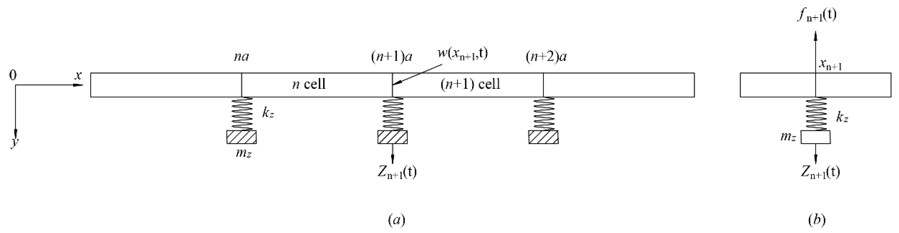
Figure 2.
(a) Illustration of a straight beam with locally resonant oscillators. (b) The sketch of the locally resonant oscillator.
Figure 2.
(a) Illustration of a straight beam with locally resonant oscillators. (b) The sketch of the locally resonant oscillator.

Figure 3.
Dispersion relationship and band gaps for a locally resonant (LR) beam.

Figure 4.
Transmission properties of the finite locally resonant (LR) beam and band gap characteristics of the corresponding infinite beam in the range of 0–800 Hz: (a) Frequency response function of the finite beam. (b) The imaginary part of wave vectors of the infinite beam.
Figure 4.
Transmission properties of the finite locally resonant (LR) beam and band gap characteristics of the corresponding infinite beam in the range of 0–800 Hz: (a) Frequency response function of the finite beam. (b) The imaginary part of wave vectors of the infinite beam.

Figure 5.
Dispersion relationship and band gaps for a locally resonant (LR) beam calculated by Timoshenko beam model (TB) and Euler-Bernoulli beam model (EB). Half of the dispersion relationship is plotted because of its symmetry.
Figure 5.
Dispersion relationship and band gaps for a locally resonant (LR) beam calculated by Timoshenko beam model (TB) and Euler-Bernoulli beam model (EB). Half of the dispersion relationship is plotted because of its symmetry.

Figure 6.
Effects of lumped mass mz on the 1st band gap: (a) Lower edge of the 1st band gap. (b) Width of the 1st band gap.
Figure 6.
Effects of lumped mass mz on the 1st band gap: (a) Lower edge of the 1st band gap. (b) Width of the 1st band gap.
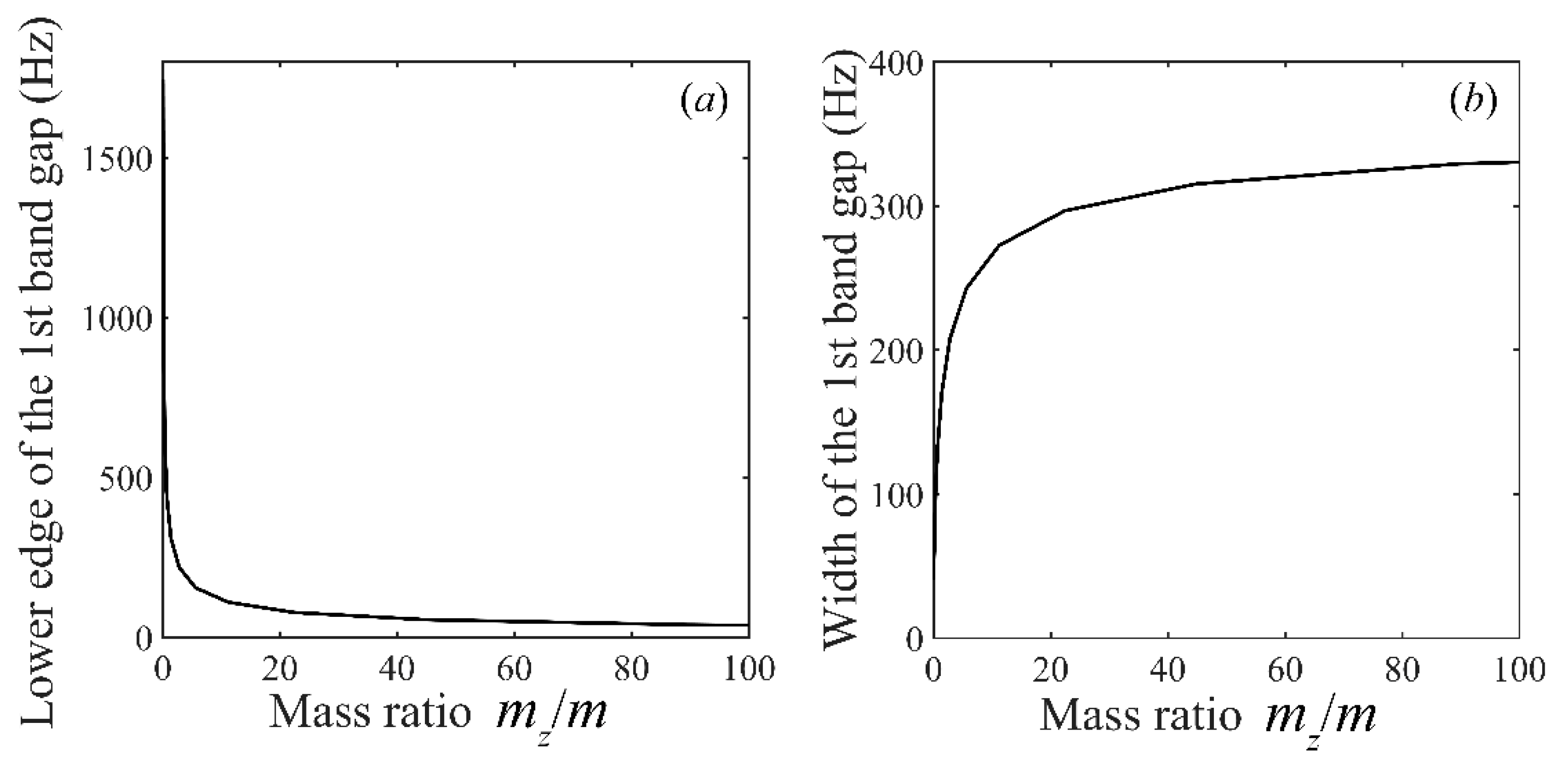
Figure 7.
Effects of the spring stiffness coefficient kz on the 1st band gap: (a) Lower edge of the 1st band gap. (b) Width of the 1st band gap.
Figure 7.
Effects of the spring stiffness coefficient kz on the 1st band gap: (a) Lower edge of the 1st band gap. (b) Width of the 1st band gap.

Figure 8.
Effects of the lattice constant a on the 1st band gap: (a) Lower edge of the 1st band gap. (b) Width of the 1st band gap.
Figure 8.
Effects of the lattice constant a on the 1st band gap: (a) Lower edge of the 1st band gap. (b) Width of the 1st band gap.


Table 1.
Material parameters.
| Parameters | Items | Values |
|---|---|---|
| ρAl | Aluminum density (kg/m3) | 2600 |
| EAl | Elastic modulus of aluminum (Pa) | 7 × 10¹⁰ |
| ρrubber | Rubber density (kg/m3) | 1300 |
| Erubber | Elastic modulus of rubber (Pa) | 7.7 × 10⁵ |
| Grubber | Shear modulus of rubber (Pa) | 2.6 × 10⁵ |
| ρCu | Copper density (kg/m3) | 8950 |
Table 2.
Fundamental frequency of a locally resonant (LR) beam.
| Wave Vector k | Present Frequency (Hz) | ||||
|---|---|---|---|---|---|
| Nx = 6 | Nx = 7 | Nx = 8 | Nx = 9 | Nx = 15 | |
| 0.0 | 0.000 | 0.000 | 0.000 | 0.000 | 0.000 |
| 0.3 | 277.547 | 277.635 | 277.638 | 277.638 | 277.638 |
| 0.5 | 304.968 | 304.972 | 304.973 | 304.973 | 304.973 |
| 0.7 | 308.056 | 308.057 | 308.057 | 308.057 | 308.057 |
| 1.0 | 308.722 | 308.722 | 308.722 | 308.722 | 308.722 |
Table 3.
The first three band gaps in a phononic crystals (PC) beam.
| Method | Band Gaps (Hz) | |||||
|---|---|---|---|---|---|---|
| First | Second | Third | ||||
| Lower | Upper | Lower | Upper | Lower | Upper | |
| Present | 616.378 | 1097.33 | 3038.92 | 6334.27 | 9601.44 | 11929.7 |
| FEM | 616.379 | 1097.33 | 3038.94 | 6334.57 | 9602.36 | 11931.3 |
| MTM | 616 | 1098 | 3038 | 6335 | 9601 | 11930 |
| PWE | 617 | 1103 | 3053 | 6358 | 9662 | 11931 |
Table 4.
Simulation times and memory required of the present method and finite element method (FEM) (Intel (R) Xeon(R) E5620 CPU, Mathematica 11.1, simulation time is in second, memory is in KB).
Table 4.
Simulation times and memory required of the present method and finite element method (FEM) (Intel (R) Xeon(R) E5620 CPU, Mathematica 11.1, simulation time is in second, memory is in KB).
| Method | Present | FEM |
|---|---|---|
| Simulation time | 8.8438 | 17.0781 |
| Memory | 154584 | 160380 |
© 2019 by the authors. Licensee MDPI, Basel, Switzerland. This article is an open access article distributed under the terms and conditions of the Creative Commons Attribution (CC BY) license (http://creativecommons.org/licenses/by/4.0/).
Share and Cite
MDPI and ACS Style
Liang, X.; Wang, T.; Jiang, X.; Liu, Z.; Ruan, Y.; Deng, Y. A Numerical Method for Flexural Vibration Band Gaps in A Phononic Crystal Beam with Locally Resonant Oscillators. Crystals 2019, 9, 293. https://doi.org/10.3390/cryst9060293
AMA Style
Liang X, Wang T, Jiang X, Liu Z, Ruan Y, Deng Y. A Numerical Method for Flexural Vibration Band Gaps in A Phononic Crystal Beam with Locally Resonant Oscillators. Crystals. 2019; 9(6):293. https://doi.org/10.3390/cryst9060293
Chicago/Turabian StyleLiang, Xu, Titao Wang, Xue Jiang, Zhen Liu, Yongdu Ruan, and Yu Deng. 2019. "A Numerical Method for Flexural Vibration Band Gaps in A Phononic Crystal Beam with Locally Resonant Oscillators" Crystals 9, no. 6: 293. https://doi.org/10.3390/cryst9060293
Note that from the first issue of 2016, this journal uses article numbers instead of page numbers. See further details here.