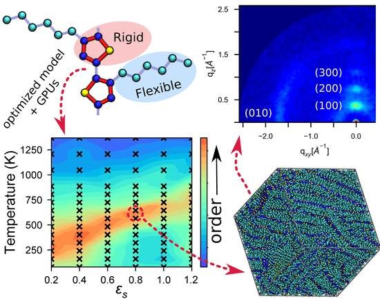
Optimization and Validation of Efficient Models for Predicting Polythiophene Self-Assembly

 , , , , and
Abstract
1. Introduction
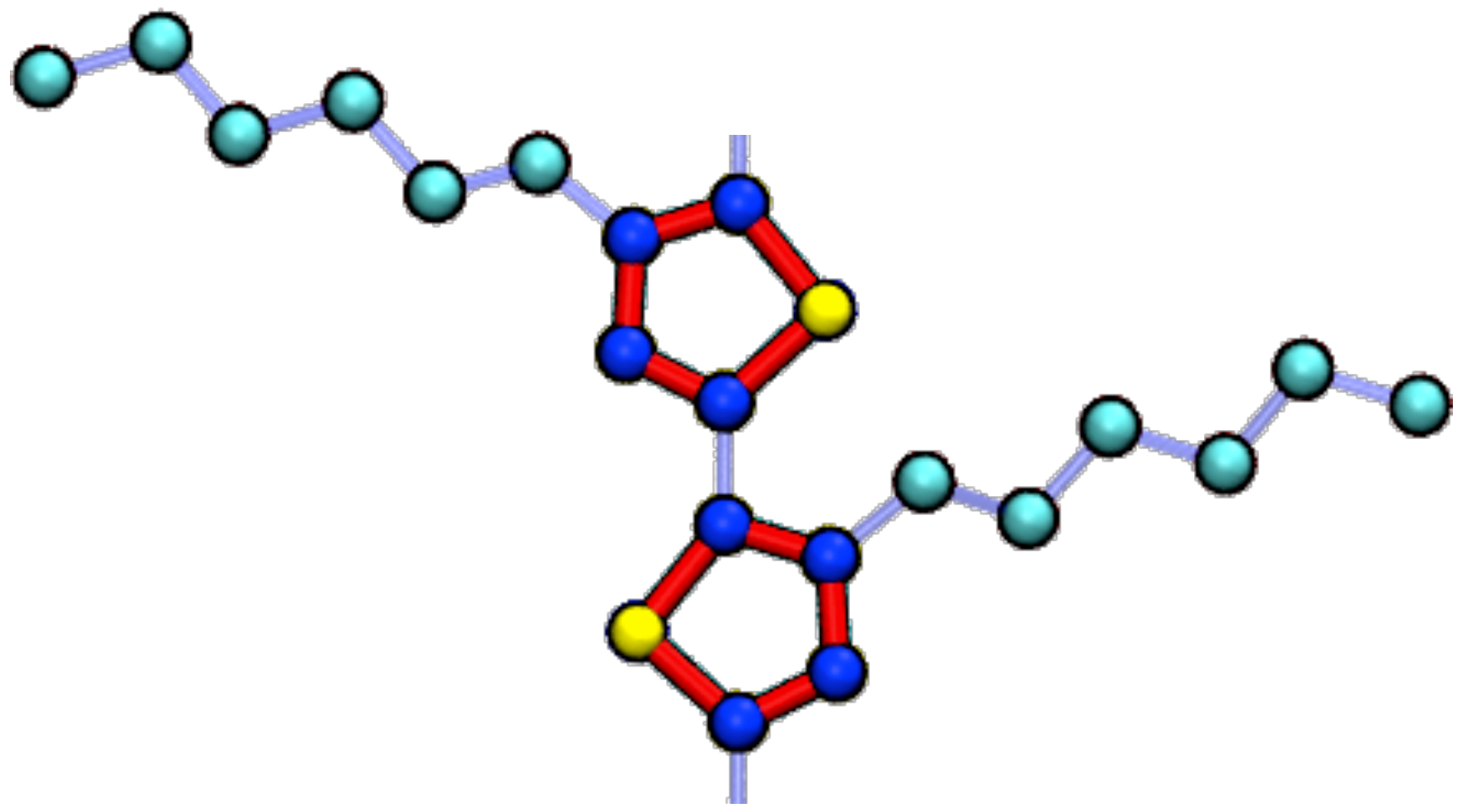
2. Model
3. Methods
3.1. Solvent Evaporation
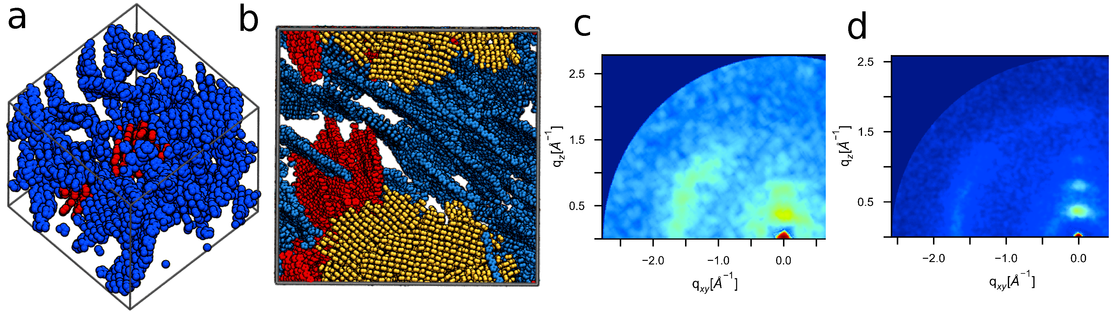
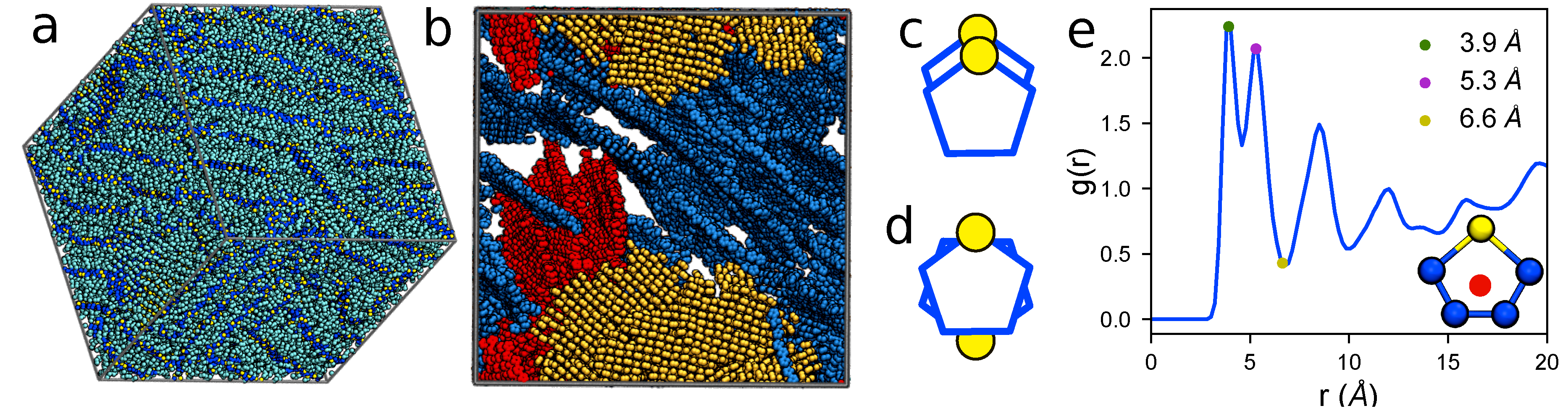
3.2. Morphology Characterization
4. Results and Discussion
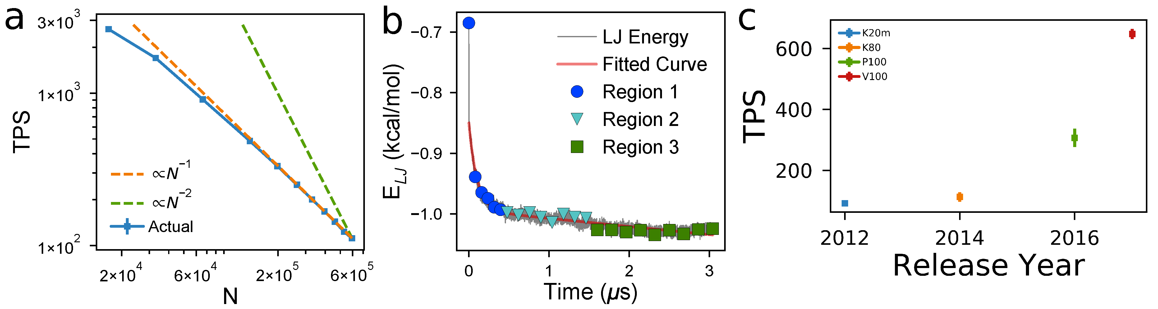
4.1. Computational Performance and Scaling
- Relaxation time: The number of timesteps that must be evaluated before the system reaches equilibrium. Larger volumes generally mean larger relaxation times because more molecules must rearrange before the system has converged to the equilibrium distribution of microstates.
- Computational performance: The number of timesteps that can be evaluated per each second that elapses on a clock on the wall, here measured as Timesteps Per Second (TPS). TPS scales between and .
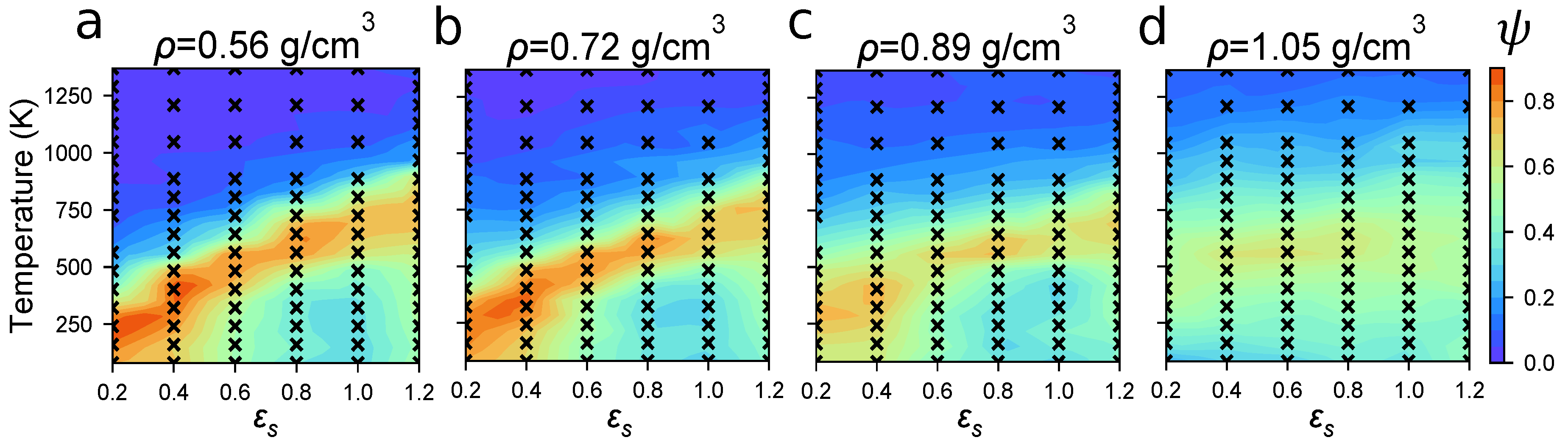
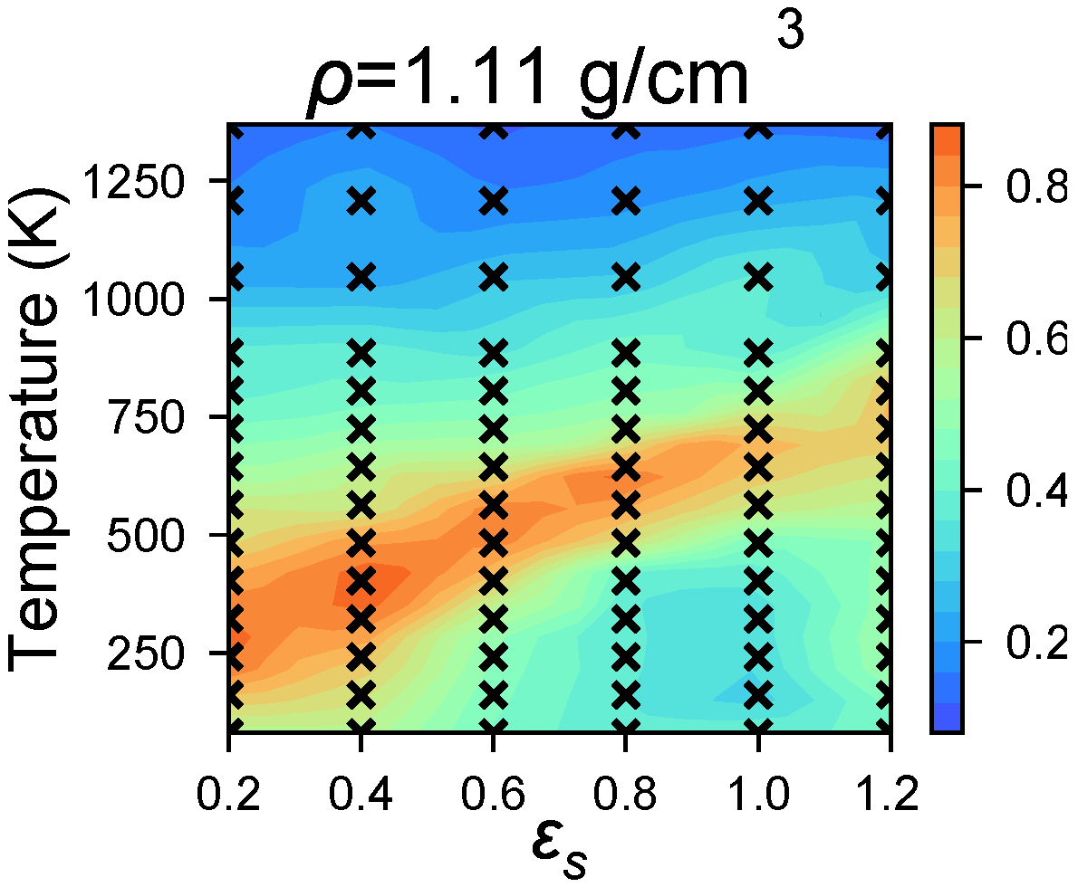
4.2. Identifying Optimal Assembly Conditions
4.3. Modeling Solvent Evaporation Facilitates Equilibration
4.4. Large Volumes Are Needed for Experimental Validation
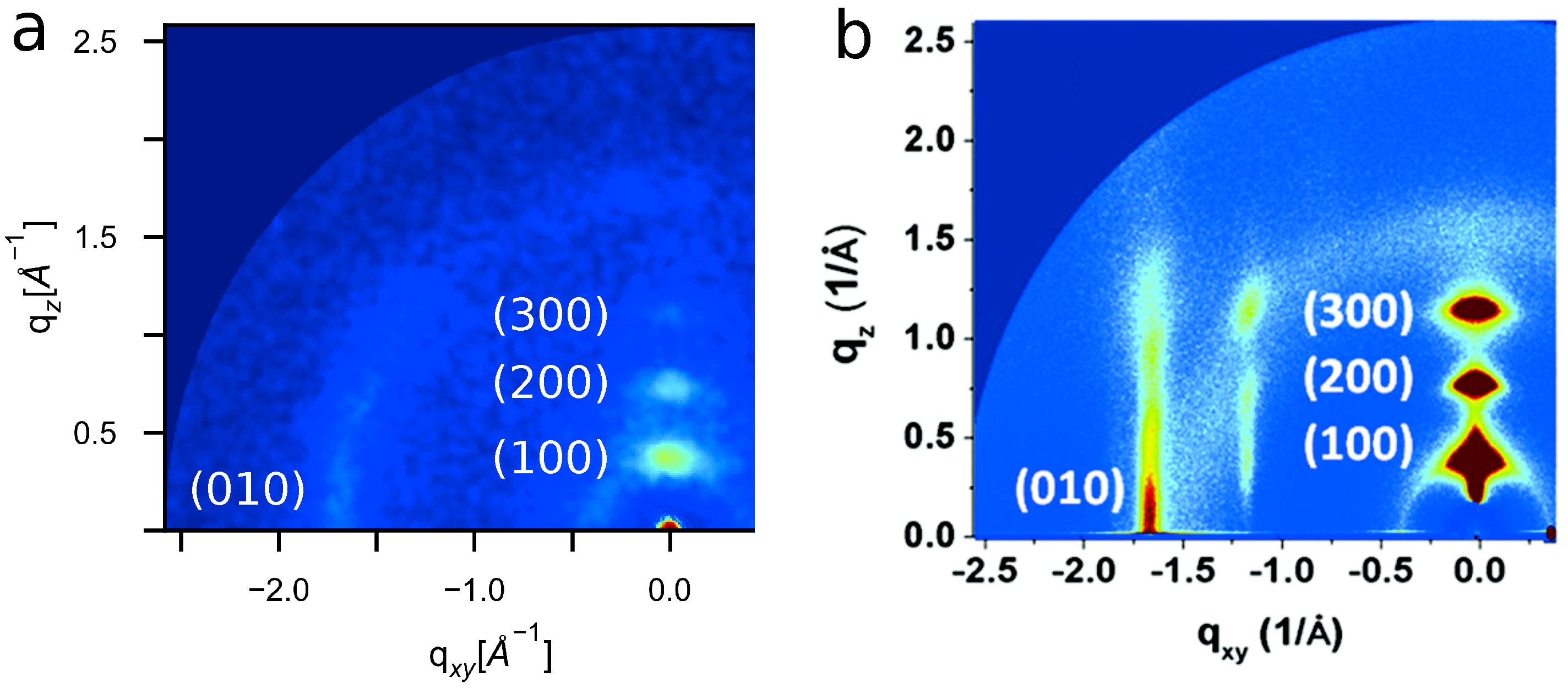
4.5. Experimental Validation of Optimized P3HT Model
5. Conclusions
- Benchmark performance to identify the system size N that is practical for equilibrating hundreds of systems.
- Generate coarse phase diagrams with these inexpensive simulations to identify rough phase boundaries and interesting structures.
- Use simulated solvent evaporation to generate morphologies at experimental densities, with sufficiently large volumes.
- Validate predictions against experimental GIXS patterns, when available.
Supplementary Materials
Author Contributions
Funding
Acknowledgments
Conflicts of Interest
Abbreviations
| 15mer | P3HT chain containing 15 monomers |
| CA | Aromatic Carbon |
| CT | Aliphatic Carbon |
| Energy Parameter | |
| Solvent Quality | |
| GIXS | Grazing Incident X-ray Scattering |
| GPU | Graphical Processing Unit |
| m | Mass |
| MD | Molecular Dynamics |
| NVT | Canonical Ensemble (constant number of particles, colume, and temperature) |
| OPLS | Optimized Potentials for Liquid Simulations |
| OPLS-UA | Optimized Potentials for Liquid Simulations - United Atom |
| OPV | Organic Photovoltaic |
| P3HT | Poly(3-hexylthiophene) |
| PCE | Power Conversion Efficiency |
| Order Parameter | |
| Density | |
| RDF | Radial Distribution Function |
| S | Sulfur |
| Lennard–Jones van der Waals radius | |
| t | Simulation Unit of Time |
| T | Temperature |
| TPS | Timesteps Per Second |
| UA | United-Atom |
References
- Espinosa, N.; Hösel, M.; Angmo, D.; Krebs, F.C. Solar Cells with One-Day Energy Payback for the Factories of the Future. Energy Environ. Sci. 2012, 5, 5117–5132. [Google Scholar] [CrossRef]
- Shaheen, S.E.; Ginley, D.S.; Jabbour, G.E. Organic-Based Photovoltaics: Toward Low-Cost Power Generation. MRS Bull. 2005, 30, 10–19. [Google Scholar] [CrossRef]
- Coakley, K.M.; McGehee, M.D. Conjugated polymer photovoltaic cells. Chem. Mater. 2004, 16, 4533–4542. [Google Scholar] [CrossRef]
- Vandewal, K.; Himmelberger, S.; Salleo, A. Structural factors that affect the performance of organic bulk heterojunction solar cells. Macromolecules 2013, 46, 6379–6387. [Google Scholar] [CrossRef]
- Dang, M.T.; Wantz, G.; Bejbouji, H.; Urien, M.; Dautel, O.J.; Vignau, L.; Hirsch, L. Polymeric Solar Cells Based on P3HT:PCBM: Role of the Casting Solvent. Sol. Energy Mater. Sol. Cells 2011, 95, 3408–3418. [Google Scholar] [CrossRef]
- Surin, M.; Leclère, P.; Lazzaroni, R.; Yuen, J.D.; Wang, G.; Moses, D.; Heeger, A.J.; Cho, S.; Lee, K. Relationship between the microscopic morphology and the charge transport properties in poly(3-hexylthiophene) field-effect transistors. J. Appl. Phys. 2006, 100, 033712. [Google Scholar] [CrossRef]
- Verploegen, E.; Mondal, R.; Bettinger, C.J.; Sok, S.; Toney, M.F.; Bao, Z. Effects of Thermal Annealing Upon the Morphology of Polymer-Fullerene Blends. Adv. Funct. Mater. 2010, 20, 3519–3529. [Google Scholar] [CrossRef]
- Park, J.H.; Kim, J.S.; Lee, J.H.; Lee, W.H.; Cho, K. Effect of Annealing Solvent Solubility on the Performance of Poly(3-hexylthiophene)/Methanofullerene Solar Cells. J. Phys. Chem. C 2009, 113, 17579–17584. [Google Scholar] [CrossRef]
- Bertho, S.; Janssen, G.; Cleij, T.J.; Conings, B.; Moons, W.; Gadisa, A.; D’Haen, J.; Goovaerts, E.; Lutsen, L.; Manca, J.; et al. Effect of temperature on the morphological and photovoltaic stability of bulk heterojunction polymer: Fullerene solar cells. Sol. Energy Mater. Sol. Cells 2008, 92, 753–760. [Google Scholar] [CrossRef]
- Clarke, T.M.; Durrant, J.R. Charge Photogeneration in Organic Solar Cells. Chem. Rev. 2010, 110, 6736–6767. [Google Scholar] [CrossRef] [PubMed]
- Camaioni, N.; Ridolfi, G.; Casalbore-Miceli, G.; Possamai, G.; Maggini, M. The Effect of a Mild Thermal Treatment on the Performance of Poly(3-alkylthiophene)/Fullerene Solar Cells. Adv. Mater. 2002, 14, 1735–1738. [Google Scholar] [CrossRef]
- Yu, G.; Gao, J.; Hummelen, J.C.; Wudl, F.; Heeger, A.J. Polymer Photovoltaic Cells: Enhanced Efficiencies via a Network of Internal Donor-Acceptor Heterojunctions. Science 1995, 270, 1789–1791. [Google Scholar] [CrossRef]
- Mazzio, K.A.; Luscombe, C.K. The future of organic photovoltaics. Chem. Soc. Rev. 2015, 44, 78–90. [Google Scholar] [CrossRef] [PubMed]
- Dang, M.T.; Hirsch, L.; Wantz, G. P3HT:PCBM, best seller in polymer photovoltaic research. Adv. Mater. 2011, 23, 3597–3602. [Google Scholar] [CrossRef] [PubMed]
- Marchiori, C.F.N.; Koehler, M. Density functional theory study of the dipole across the P3HT:PCBM complex: The role of polarization and charge transfer. J. Phys. D Appl. Phys. 2014, 47, 215104. [Google Scholar] [CrossRef]
- Lan, Y.K.; Huang, C.I. A Theoretical Study of the Charge Transfer Behavior of the Highly Regioregular Poly-3-hexylthiophene in the Ordered State. J. Phys. Chem. B 2008, 112, 14857–14862. [Google Scholar] [CrossRef] [PubMed]
- Xie, W.; Sun, Y.Y.; Zhang, S.B.; Northrup, J.E. Structure and sources of disorder in poly(3-hexylthiophene) crystals investigated by density functional calculations with van der Waals interactions. Phys. Rev. B Condens. Matter Mater. Phys. 2011, 83, 184117. [Google Scholar] [CrossRef]
- Peumans, P.; Uchida, S.; Forrest, S.R. Efficient bulk heterojunction photovoltaic cells using small-molecular-weight organic thin films. Nature 2003, 425, 158–162. [Google Scholar] [CrossRef] [PubMed]
- Groves, C.; Kimber, R.G.E.; Walker, A.B. Simulation of Loss Mechanisms in Organic Solar Cells: A Description of the Mesoscopic Monte Carlo Technique and an Evaluation of the First Reaction Method. J. Chem. Phys. 2010, 133, 144110. [Google Scholar] [CrossRef] [PubMed]
- Henderson, I.C.; Clarke, N. On Modelling Surface Directed Spinodal Decomposition. Macromol. Theory Simul. 2005, 14, 435–443. [Google Scholar] [CrossRef]
- Fukuda, J.I.; Yoneya, M.; Yokoyama, H. Numerical treatment of the dynamics of a conserved order parameter in the presence of walls. Phys. Rev. E 2006, 73, 066706. [Google Scholar] [CrossRef] [PubMed]
- Lyons, B.P.; Clarke, N.; Groves, C. The Quantitative Effect of Surface Wetting Layers on the Performance of Organic Bulk Heterojunction Photovoltaic Devices. J. Phys. Chem. C 2011, 115, 22572–22577. [Google Scholar] [CrossRef]
- Wodo, O.; Ganapathysubramanian, B. Modeling morphology evolution during solvent-based fabrication of organic solar cells. Comput. Mater. Sci. 2012, 55, 113–126. [Google Scholar] [CrossRef]
- Wodo, O.; Tirthapura, S.; Chaudhary, S.; Ganapathysubramanian, B. A graph-based formulation for computational characterization of bulk heterojunction morphology. Org. Electron. 2012, 13, 1105–1113. [Google Scholar] [CrossRef]
- Van, E.; Jones, M.; Jankowski, E.; Wodo, O. Using graphs to quantify energetic and structural order in semicrystalline oligothiophene thin films. Mol. Syst. Des. Eng. 2018, 1, 273–277. [Google Scholar] [CrossRef]
- Huang, D.M.; Faller, R.; Do, K.; Moulé, A.J. Coarse-Grained Computer Simulations of Polymer/Fullerene Bulk Heterojunctions for Organic Photovoltaic Applications. J. Chem. Theory Comput. 2010, 6, 526–537. [Google Scholar] [CrossRef] [PubMed]
- Ismail, A.E.; Stephanopoulos, G.; Rutledge, G.C. Topological coarse graining of polymer chains using wavelet-accelerated Monte Carlo. II. Self-avoiding chains. J. Chem. Phys. 2005, 122, 234902. [Google Scholar] [CrossRef] [PubMed]
- Jankowski, E.; Marsh, H.S.; Jayaraman, A. Computationally Linking Molecular Features of Conjugated Polymers and Fullerene Derivatives to Bulk Heterojunction Morphology. Macromolecules 2013, 46, 5775–5785. [Google Scholar] [CrossRef]
- Van Lehn, R.C.; Atukorale, P.U.; Carney, R.P.; Yang, Y.S.; Stellacci, F.; Irvine, D.J.; Alexander-Katz, A. Effect of Particle Diameter and Surface Composition on the Spontaneous Fusion of Monolayer-Protected Gold Nanoparticles with Lipid Bilayers. Nano Lett. 2013, 13, 4060–4067. [Google Scholar] [CrossRef] [PubMed]
- Gross, J.; Ivanov, M.; Janke, W. Comparing atomistic and coarse-grained simulations of P3HT. J. Phys. Conf. Ser. 2016, 750, 012009. [Google Scholar] [CrossRef]
- Jones, M.L.; Huang, D.M.; Chakrabarti, B.; Groves, C. Relating Molecular Morphology to Charge Mobility in Semicrystalline Conjugated Polymers. J. Phys. Chem. C 2016, 120, 4240–4250. [Google Scholar] [CrossRef]
- Scherer, C.; Andrienko, D. Comparison of systematic coarse-graining strategies for soluble conjugated polymers. Eur. Phys. J. Spec. Top. 2016, 225, 1441–1461. [Google Scholar] [CrossRef]
- Lee, C.K.; Pao, C.W.; Chu, C.W. Multiscale molecular simulations of the nanoscale morphologies of P3HT:PCBM blends for bulk heterojunction organic photovoltaic cells. Energy Environ. Sci. 2011, 4, 4124. [Google Scholar] [CrossRef]
- Carrillo, J.M.Y.; Kumar, R.; Goswami, M.; Sumpter, B.G.; Brown, W.M. New insights into the dynamics and morphology of P3HT:PCBM active layers in bulk heterojunctions. Phys. Chem. Chem. Phys. 2013, 15, 17873. [Google Scholar] [CrossRef] [PubMed]
- Jones, M.L.; Jankowski, E. Computationally connecting organic photovoltaic performance to atomistic arrangements and bulk morphology. Mol. Simul. 2017, 43, 756–773. [Google Scholar] [CrossRef]
- Loser, S.; Lou, S.J.; Savoie, B.M.; Bruns, C.J.; Timalsina, A.; Leonardi, M.J.; Smith, J.; Harschneck, T.; Turrisi, R.; Zhou, N.; et al. Systematic evaluation of structure–property relationships in heteroacene—Diketopyrrolopyrrole molecular donors for organic solar cells. J. Mater. Chem. A 2017, 5, 9217–9232. [Google Scholar] [CrossRef]
- Bhatta, R.S.; Yimer, Y.Y.; Perry, D.S.; Tsige, M. Improved Force Field for Molecular Modeling of Poly(3-hexylthiophene). J. Phys. Chem. B 2013, 117, 10035–10045. [Google Scholar] [CrossRef] [PubMed]
- Obata, S.; Shimoi, Y. Control of molecular orientations of poly(3-hexylthiophene) on self-assembled monolayers: Molecular dynamics simulations. Phys. Chem. Chem. Phys. 2013, 15, 9265–9270. [Google Scholar] [CrossRef] [PubMed]
- Jackson, N.E.; Kohlstedt, K.L.; Savoie, B.M.; Olvera de la Cruz, M.; Schatz, G.C.; Chen, L.X.; Ratner, M.A. Conformational Order in Aggregates of Conjugated Polymers. J. Am. Chem. Soc. 2015, 137, 6254–6262. [Google Scholar] [CrossRef] [PubMed]
- Borzdun, N.I.; Larin, S.V.; Falkovich, S.G.; Nazarychev, V.M.; Volgin, I.V.; Yakimansky, A.V.; Lyulin, A.V.; Negi, V.; Bobbert, P.A.; Lyulin, S.V. Molecular dynamics simulation of poly(3-hexylthiophene) helical structure In Vacuo and in amorphous polymer surrounding. J. Polym. Sci. Part B Polym. Phys. 2016, 54, 2448–2456. [Google Scholar] [CrossRef]
- Xuan, P.; Zheng, Y.; Sarupria, S.; Apon, A. SciFlow: A dataflow-driven model architecture for scientific computing using Hadoop. In Proceedings of the 2013 IEEE International Conference on Big Data, Silicon Valley, CA, USA, 6–9 October 2013; pp. 36–44. [Google Scholar] [CrossRef]
- DeLongchamp, D.M.; Kline, R.J.; Herzing, A. Nanoscale Structure Measurements for Polymer-Fullerene Photovoltaics. Energy Environ. Sci. 2012, 5, 5980–5993. [Google Scholar] [CrossRef]
- Chen, W.; Nikiforov, M.P.; Darling, S.B. Morphology characterization in organic and hybrid solar cells. Energy Environ. Sci. 2012, 5, 8045–8074. [Google Scholar] [CrossRef]
- Coffey, D.C.; Reid, O.G.; Rodovsky, D.B.; Bartholomew, G.P.; Ginger, D.S. Mapping local photocurrents in polymer/fullerene solar cells with photoconductive atomic force microscopy. Nano Lett. 2007, 7, 738–744. [Google Scholar] [CrossRef] [PubMed]
- Martin, M.G.; Siepmann, J.I. Transferable Potentials for Phase Equilibria. 1. United-Atom Description of n-Alkanes. J. Phys. Chem. B 1998, 102, 2569–2577. [Google Scholar] [CrossRef]
- Jorgensen, W.L.; Tirado-Rives, J. The OPLS [Optimized Potentials for Liquid Simulations] Potential Functions for Proteins, Energy Minimizations for Crystals of Cyclic Peptides and Crambin. J. Am. Chem. Soc. 1988, 110, 1657–1666. [Google Scholar] [CrossRef] [PubMed]
- Kim, H.; Bedrov, D.; Smith, G.D.; City, S.L. Molecular Dynamics Simulation Study of the Influence of Cluster Geometry on Formation of C 60 Fullerene Clusters in Aqueous Solution. J. Chem. Theory Comput. 2008, 4, 335–340. [Google Scholar] [CrossRef] [PubMed]
- Chen, C.; Depa, P.; Sakai, V.G.; Maranas, J.K.; Lynn, J.W.; Peral, I.; Copley, J.R.D. A Comparison of United Atom, Explicit Atom, and Coarse-grained Simulation Models for poly(ethylene oxide). J. Chem. Phys. 2006, 124, 234901. [Google Scholar] [CrossRef] [PubMed]
- Henry, M.M.; Jones, M.L.; Oosterhout, S.D.; Braunecker, W.A.; Kemper, T.W.; Larsen, R.E.; Kopidakis, N.; Toney, M.F.; Olson, D.C.; Jankowski, E. Simplified Models for Accelerated Structural Prediction of Conjugated Semiconducting Polymers. J. Phys. Chem. C 2017, 121, 26528–26538. [Google Scholar] [CrossRef]
- Miller, E.D.; Jones, M.L.; Jankowski, E. Enhanced Computational Sampling of Perylene and Perylothiophene Packing with Rigid-Body Models. ACS Omega 2017, 2, 353–362. [Google Scholar] [CrossRef]
- Yoon, D.Y.; Smith, G.D.; Matsuda, T. A Comparison in Simulations of a United Atom and an Explicit of polymethylene Atom Model. J. Chem. Phys. 1993, 98, 10037–10043. [Google Scholar] [CrossRef]
- Jorgensen, W.L.; Madura, J.D.; Swenson, C.J. Optimized Intermolecular Potential Functions for Liquid Hydrocarbons. J. Am. Chem. Soc. 1984, 106, 6638–6646. [Google Scholar] [CrossRef]
- Nguyen, T.D.; Phillips, C.L.; Anderson, J.A.; Glotzer, S.C. Rigid Body Constraints Realized in Massively-parallel Molecular Dynamics on Graphics Processing Units. Comput. Phys. Commun. 2011, 182, 2307–2313. [Google Scholar] [CrossRef]
- Wu, G.; Robertson, D.H.; Brooks, C.L.; Vieth, M. Detailed analysis of grid-based molecular docking: A case study of CDOCKER-A CHARMm-based MD docking algorithm. J. Comput Chem. 2003, 24, 1549–1562. [Google Scholar] [CrossRef] [PubMed]
- Izvekov, S.; Parrinello, M.; Burnham, C.J.; Voth, G.A. Effective force fields for condensed phase systems from ab initio molecular dynamics simulation: A new method for force-matching. J. Chem. Phys. 2004, 120, 10896–10913. [Google Scholar] [CrossRef] [PubMed]
- Topf, M.; Lasker, K.; Webb, B.; Wolfson, H.; Chiu, W.; Sali, A. Protein Structure Fitting and Refinement Guided by Cryo-EM Density. Structure 2008, 16, 295–307. [Google Scholar] [CrossRef] [PubMed]
- Anderson, J.A.; Lorenz, C.D.; Travesset, A. General Purpose Molecular Dynamics Simulations Fully Implemented on Graphics Processing Units. J. Comput. Phys. 2008, 227, 5342–5359. [Google Scholar] [CrossRef]
- Glaser, J.; Nguyen, T.D.; Anderson, J.A.; Lui, P.; Spiga, F.; Millan, J.A.; Morse, D.C.; Glotzer, S.C. Strong Scaling of General-purpose Molecular Dynamics Simulations on GPUs. Comput. Phys. Commun. 2014, 192, 97–107. [Google Scholar] [CrossRef]
- Miller, E.D.; Jones, M.L.; Henry, M.M.; Jankowski, E. Poly-(3-hexylthiophene) Model and Code for Molecular Dynamic Simulations. 2018. Available online: https://zenodo.org/record/1420535#.W_Y0jcQRWUk (accessed on 22 November 2018).
- Miller, E.D.; Jones, M.L.; Henry, M.M.; Jankowski, E. Molecular Dynamics Data for Optimization and Validation of Modeling Techniques for Predicting Structures and Charge Mobilities of P3HT. 2018. Available online: https://scholarworks.boisestate.edu/cme_lab/4/ (accessed on 22 November 2018).
- Hoover, W.G. Canonical Dynamics: Equilibrium Phase-space Distributions. Phys. Rev. A 1985, 31, 1695–1697. [Google Scholar] [CrossRef]
- Swope, W.C.; Andersen, H.C.; Berens, P.H.; Wilson, K.R. A Computer Simulation Method for the Calculation of Equilibrium Constants for the Formation of Physical Clusters of Molecules: Application to Small Water Clusters. J. Chem. Phys. 1982, 76, 637–649. [Google Scholar] [CrossRef]
- Klein, C.; Sallai, J.; Jones, T.J.; Iacovella, C.R.; McCabe, C.; Cummings, P.T. A Hierarchical, Component Based Approach to Screening Properties of Soft Matter. In Foundations of Molecular Modeling and Simulation; Springer: Singapore, 2016. [Google Scholar]
- Marsh, H.S.; Jankowski, E.; Jayaraman, A. Controlling the Morphology of Model Conjugated Thiophene Oligomers through Alkyl Side Chain Length, Placement, and Interactions. Macromolecules 2014, 47, 2736–2747. [Google Scholar] [CrossRef]
- Newbloom, G.M.; Weigandt, K.M.; Pozzo, D.C. Structure and property development of poly(3-hexylthiophene) organogels probed with combined rheology, conductivity and small angle neutron scattering. Soft Matter 2012, 8, 8854. [Google Scholar] [CrossRef]
- Roux, B.; Simonson, T. Implicit solvent models. Biophys. Chem. 1999, 78, 1–20. [Google Scholar] [CrossRef]
- Feig, M.; Brooks, C.L. Recent advances in the development and application of implicit solvent models in biomolecule simulations. Curr. Opin. Struct. Biol. 2004, 14, 217–224. [Google Scholar] [CrossRef] [PubMed]
- Shin, H.; Pascal, T.A.; Goddard, W.A.; Kim, H. Scaled effective solvent method for predicting the equilibrium ensemble of structures with analysis of thermodynamic properties of amorphous polyethylene glycol-water mixtures. J. Phys. Chem. B 2013, 117, 916–927. [Google Scholar] [CrossRef] [PubMed]
- Damasceno, P.F.; Engel, M.; Glotzer, S.C. Predictive Self-Assembly of Polyhedra into Complex Structures. Science 2012, 337, 453–457. [Google Scholar] [CrossRef] [PubMed]
- Miller, E.D.; Henry, M.M.; Jankowski, E. Diffractometer (Version 1.0). Zenodo. 2018. Available online: http://doi.org/10.5281/zenodo.1340716 (accessed on 6 August 2018).
- Ingólfsson, H.I.; Lopez, C.A.; Uusitalo, J.J.; de Jong, D.H.; Gopal, S.M.; Periole, X.; Marrink, S.J. The power of coarse graining in biomolecular simulations. Wiley Interdiscip. Rev. Comput. Mol. Sci. 2014, 4, 225–248. [Google Scholar] [CrossRef] [PubMed]
- Phillips, C.L.; Voth, G.A. Discovering Crystals Using Shape Matching and Machine Learning. Soft Matter 2013, 9, 8552. [Google Scholar] [CrossRef]
- Sidky, H.; Colón, Y.J.; Helfferich, J.; Sikora, B.J.; Bezik, C.; Chu, W.; Giberti, F.; Guo, A.Z.; Jiang, X.; Lequieu, J.; et al. SSAGES: Software Suite for Advanced General Ensemble Simulations. J. Chem. Phys. 2018, 148, 044104. [Google Scholar] [CrossRef] [PubMed]
- Ko, S.; Hoke, E.T.; Pandey, L.; Hong, S.; Mondal, R.; Risko, C.; Yi, Y.; Noriega, R.; McGehee, M.D.; Brédas, J.L.; et al. Controlled conjugated backbone twisting for an increased open-circuit voltage while having a high short-circuit current in poly(hexylthiophene) derivatives. J. Am. Chem. Soc. 2012, 134, 5222–5232. [Google Scholar] [CrossRef] [PubMed]
- Lane, T.J.; Shukla, D.; Beauchamp, K.A.; Pande, V.S. To milliseconds and beyond: Challenges in the simulation of protein folding. Curr. Opin. Struct. Biol. 2013, 23, 58–65. [Google Scholar] [CrossRef] [PubMed]
- Towns, J.; Cockerill, T.; Dahan, M.; Foster, I.; Gaither, K.; Grimshaw, A.; Hazlewood, V.; Lathrop, S.; Lifka, D.; Peterson, G.D.; et al. XSEDE: Accelerating Scientific Discovery. Comput. Sci. Eng. 2014, 16, 62–74. [Google Scholar] [CrossRef]


| Bead Type | (Å) | (kcal/mol) | m (amu) |
|---|---|---|---|
| CA | 3.436 | 0.11 | 13.0 |
| CT | 3.905 | 0.17 | 15.0 |
| S | 3.436 | 0.32 | 32.0 |
© 2018 by the authors. Licensee MDPI, Basel, Switzerland. This article is an open access article distributed under the terms and conditions of the Creative Commons Attribution (CC BY) license (http://creativecommons.org/licenses/by/4.0/).
Share and Cite
Miller, E.D.; Jones, M.L.; Henry, M.M.; Chery, P.; Miller, K.; Jankowski, E. Optimization and Validation of Efficient Models for Predicting Polythiophene Self-Assembly. Polymers 2018, 10, 1305. https://doi.org/10.3390/polym10121305
Miller ED, Jones ML, Henry MM, Chery P, Miller K, Jankowski E. Optimization and Validation of Efficient Models for Predicting Polythiophene Self-Assembly. Polymers. 2018; 10(12):1305. https://doi.org/10.3390/polym10121305
Chicago/Turabian StyleMiller, Evan D., Matthew L. Jones, Michael M. Henry, Paul Chery, Kyle Miller, and Eric Jankowski. 2018. "Optimization and Validation of Efficient Models for Predicting Polythiophene Self-Assembly" Polymers 10, no. 12: 1305. https://doi.org/10.3390/polym10121305
APA StyleMiller, E. D., Jones, M. L., Henry, M. M., Chery, P., Miller, K., & Jankowski, E. (2018). Optimization and Validation of Efficient Models for Predicting Polythiophene Self-Assembly. Polymers, 10(12), 1305. https://doi.org/10.3390/polym10121305