Determine Mesh Size through Monomer Mean-Square Displacement


School of Physics, Southeast University, Nanjing 211189, China
Polymers 2019, 11(9), 1405; https://doi.org/10.3390/polym11091405
Submission received: 14 January 2019
/
Revised: 23 August 2019
/
Accepted: 23 August 2019
/
Published: 27 August 2019
(This article belongs to the Special Issue Theory and Simulations of Entangled Polymers)
Abstract
:A dynamic method to determine the main parameter of the tube theory through monomer mean-square displacement is discussed in this paper. The tube step length can be measured from the intersection of the slope- line and the slope- line in log-log plot, and the tube diameter can be obtained by recording the time at which data start to leave the slope- regime. According to recent simulation data, the ratio of the tube step length to the tube diameter was found to be about 2 for different entangled polymer systems. Since measuring the tube diameter does not require data to reach the slope- regime, this could be the best way to find the entanglement length from microscopic consideration.
1. Introduction
Modern theories of polymer dynamics and rheology describe the universal aspects of the viscoelastic behavior based on the idea that molecular entanglements confine individual filaments to a one-dimensional, diffusive dynamics (reptation) in tube-like regions in space [1]. Entanglements are transient topological constraints arising from the restriction that the backbones of fluctuating chain molecules cannot cut through each other [2,3]. Since linear polymers are strongly interpenetrating, these constraints dominate the long-time dynamics of high molecular weight polymers, and entanglements strongly slow down the relaxation. A characteristic feature is subdiffusion regime in monomer mean-square displacement (MSD), which is even slower than the free three-dimensional Rouse motion [2,3].
Mesh size is one of most important quantities in tube theory. A quick method to predict mesh size is required and it should be easy to realize in computer simulations. Based on the concept of primitive path, the topological approach proposed by Everaers et al. is the so-called primitive path analysis (PPA), which can directly provide the statistical information of the primitive path mesh [4,5]. To obtain the precise results from PPA, one need to extrapolate the PPA results to infinite long chain [6], and this extrapolated result given by PPA has been verified by stress relaxation data [7]. An alternative method by using the monomer MSD was firstly proposed by Likhtman and McLeish [8]. This method is based on the scaling argument of the behaviors of MSD in different time regimes. Therefore, it is also subject to sufficient long chain system. Seeking a quick and easy method to determine the mesh size in medium-length entangled system is the aim of this paper.
The remainder of the paper is structured as follows. In Section 2, the difference between tube step length (TSL) and tube diameter (TD) is clarified. Section 3 is devoted to the calculation of the monomer MSD of entangled chain. Descriptions of determining the mesh size through MSD are presented in Section 4, and the ratio between these two quantities is given in Section 5. Finally, a brief summary is given in the last section.
2. Tube Step Length and Tube Diameter
In an entangled polymer melt, each polymer chain consists of N Kuhn beads and is confined in a tube formed by all other surrounding chains [2,9]. The center line of the tube is called primitive path (PP) which can be thought as a random Kuhn walk containing Z steps with the TSL a. The mean-square end-to-end distance of the tube should be equal to the mean-square end-to-end distance of the chain, . The entanglement length is defined as the number of monomers in a tube segment, . and denote the Rouse time and the disentanglement time respectively. The entanglement time is defined as the Rouse time of the chain segment between entanglements, .
The concept of TSL a is sometimes confused with TD . TD specifies the range that a monomer can move perpendicularly to the tube. TSL and TD are two different concepts, although both share the same magnitude (see Figure 1). The linear rheological properties of an entangled melt are mainly determined by the TSL [2,8], while the mobility of nonsticky nanoparticles is governed by the ratio of the nanoparticle diameter to the TD [10,11,12,13,14,15].
3. Monomer Displacement in Entangled Linear Melts
The mean-square displacement (MSD) of a monomer in a melt is given by
where and denote the number of polymer chains and the position of the monomer, respectively. At a time smaller than the entanglement time , can be calculated by the three-dimensional Rouse model [16],
At later time , the motion of the Kuhn segment perpendicular to the tube is suppressed by the constraints, and the motion longitudinal to the primitive path can be calculated by the one-dimensional Rouse model with both chain ends stretched by an entropic force [2]. The curvilinear MSD is
is just one third of because only the one-dimensional longitudinal motion is allowed inside the tube in three-dimensional space. Thus, the motion perpendicular to the tube before the polymer chain meets the tube can be calculated by
Since is longitudinal, the MSD in three-dimensional space is . Therefore, at time ,
The prefactor in the last equation appears since the distribution of segment displacement alone the tube is Gaussian.
4. Determination of Mesh Size
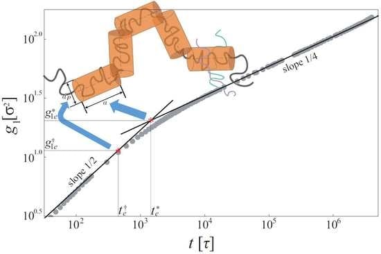
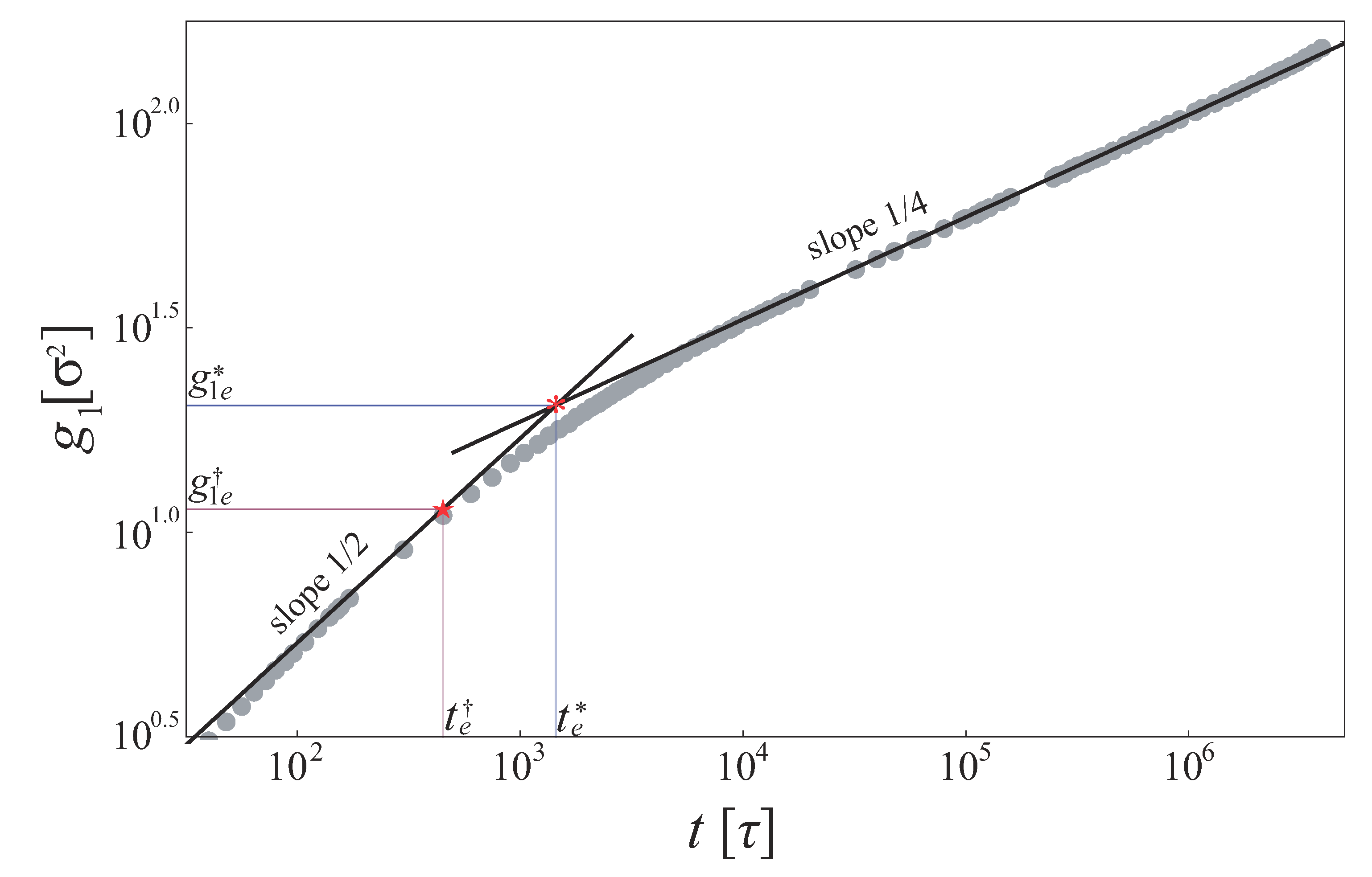
In the log-log plot, the data can be fitted by straight lines in different time regimes ( and ) (see Figure 2). One can obtain an intersecting point close to the entanglement time (the point marked by a red asterisk in Figure 2).
Therefore, TSL a, entanglement time and entanglement length can be obtain using this intersecting point,
This dynamic method to determine TSL was firstly proposed by Likhtman and McLeish with a slightly different prefactor [8]. The entanglement length derived here is times larger than the original prediction of reference [17].
Figure 2 shows the the most refined simulation data [18] of the Kremer–Grest model (KGM) [19] with the bond bending interactions parameter [18]. and are estimated as and using this method, where and are Lennard–Jones time unit and length unit, respectively. Using Equation (9), the entanglement length is estimated as 33, which is consistent with the PPA result (28).
There is a drawback, however: the slope- regime of the data is not easy to reach unless the simulated chains are extremely long. It is more common that the slop of data lies between 0.25 and 0.5 in the time regime of . Stephanou et al. proposed an another method to estimate the TD by using data which do not need to reach the slope- regime [20,21,22]. Instead of finding the intersecting point between the slope- regime and the slope- regime, they recorded the time at which the data start to leave the initial slope- regime (see the point marked by a red pentagram in Figure 2). They supposed that, at time , the monomer starts to feel the tube constraints, and the monomer displacement perpendicularly to the PP is comparable to the squared tube radius . Thus,
The prefactor above rises from the two-dimensional Gaussian distribution [23]. The TD becomes
5. The Ratio of TSL to TD
Based on the methods introduced in the last section, both TSL and TD can be estimated from monomer MSD data. Using Equation (8) and (11), the ratio of TSL to TD can be measured by
The parameters for linear polymer melts measured via MSD are given in Table 1. The measured results show the ratio for different polymers.
The theoretical explanation for the ratio of 2 was given by Öttinger [30]. He adopted the Porod–Kratky wormlike chain model [31] for modeling entangled polymer chains. He showed that, for very long chains, the Kuhn length of the primitive chain turns out to be twice the TD (see Equation (47) in [30]).
It is well known that the PPA measurements (using Kröger’s Z algorithm [5] or CReTA algorithm [32]) show that the Kuhn length of the PP a is about twice as great as the mesh size of the PP network [6,32,33,34,35]. Everaers drew a particular analogy between the PP network and the phantom network, and he offered a physical interpretation of the ratio 2 [36]. Everaers’ argument is as follows: By treating the kinks or topological constraints of the PP network as the crosslinks of the phantom network model, the shear modulus is
with the presence of crosslink fluctuations, where , f and are the monomer density, arm number of the junction point and the number of monomers between the adjacent kinks, respectively. On the other hand, the melt plateau modulus is
within the affine approximation, where is the number of monomers per PP Kuhn length. Since the kinks of the PP network can be thought as four-arm branch points () and should be identical to in the rheological experiments, we have
by construction.
It is not easy to understand why the ratio of TSL to TD should be 2 due to the obscurity of the concept of tube. To get around the obscure picture of tube, Likhtman et al. proposed a simple model of a single entangled chain in a cubic lattice of line obstacles which is called grid model [37]. The grid model is intuitive and one could expect a perfect correspondence between this model and tube theory. One might anticipate that the TSL should be equal to the grid size. However, they found that the TSL measured by PPA in this model is also twice as large as the grid spacing for large grids.
As mentioned in Section 2, the mobility of non-sticky nanoparticles is governed by the ratio of nanoparticle diameter to TD . Small particles () are only affected by the monomer motion, while large particles () are affected by the mesh formed by entangled polymers [10,11,12,13,14]. Thus, one can expect that the diffusion coefficient of the nanoparticles decreases as the increase of by
Recent simulation [15] shows that
in which c is a fitting parameter and a is the TSL measured by PPA. The best-fit result is . Therefore, comparing Equation (17) with Equation (16), the observation of this paper that is verified by the nanoparticle motion in entangled polymer melts.
If holds for all the situations, it becomes much easier to determine mesh size through monomer MSD. As discussed in Section 4, it is much easier to estimate TD than TSL a, because measuring a requires the slope- regime of MSD while measuring does not. Hence, one can measure TD by simulating short chain system (longer than ), and obtain TSL immediately by using the relation . This method to determine tube mesh size through MSD shown in this paper is more robust than other methods [8]. For example, one can also estimate the entanglement length by using the plateau modulus, . However, this method has systematic error that comes from no-naffine deformation and the fluctuation of entanglement points [8]. Another method to determine the entanglement length is PPA. However, the results given by PPA are not reliable unless they are extrapolated to infinite long chain [6].
6. Summary
In this paper, we fully discuss a dynamic method to define the main parameter of the tube theory through monomer MSD . The TSL can be measured from the intersection of the fitting line and the fitting line in log-log plot. The TD can be obtained by recording the time at which data start to leave the regime. Using this method, simulation data show that the TSL is twice as large as the TD.
Funding
This research received no external funding.
Conflicts of Interest
The author declares no conflict of interest.
References and Note
- De Gennes, P. Scaling Concepts in Polymer Physics; Cornell University Press: Ithaca, NY, USA, 1979. [Google Scholar]
- Doi, M.; Edwards, S. The Theory of Polymer Dynamics; Oxford University Press: Oxford, UK, 1986. [Google Scholar]
- Rubinstein, M.; Colby, R.H. Polymer Physics; Oxford University Press: New York, NY, USA, 2003. [Google Scholar]
- Everaers, R.; Sukumaran, S.K.; Grest, G.S.; Svaneborg, C.; Sivasubramanian, A.; Kremer, K. Rheology and microscopic topology of entangled polymeric liquids. Science 2004, 303, 823–826. [Google Scholar] [CrossRef]
- Kröger, M. Shortest multiple disconnected path for the analysis of entanglements in two-and three-dimensional polymeric systems. Comput. Phys. Commun. 2005, 168, 209–232. [Google Scholar] [CrossRef]
- Hoy, R.S.; Foteinopoulou, K.; Kröger, M. Topological analysis of polymeric melts: Chain-length effects and fast-converging estimators for entanglement length. Phys. Rev. E 2009, 80, 031803. [Google Scholar] [CrossRef] [Green Version]
- Hou, J.X.; Svaneborg, C.; Everaers, R.; Grest, G.S. Stress relaxation in entangled polymer melts. Phys. Rev. Lett. 2010, 105, 068301. [Google Scholar] [CrossRef]
- Likhtman, A.E.; McLeish, T.C.B. Quantitative theory for linear dynamics of linear entangled polymers. Macromolecules 2002, 35, 6332–6343. [Google Scholar] [CrossRef]
- De Gennes, P.G. Reptation of a polymer chain in the presence of fixed obstacles. J. Chem. Phys. 1971, 55, 572–579. [Google Scholar] [CrossRef]
- Yamamoto, U.; Schweizer, K.S. Theory of nanoparticle diffusion in unentangled and entangled polymer melts. J. Chem. Phys. 2011, 135, 224902. [Google Scholar] [CrossRef]
- Cai, L.H.; Panyukov, S.; Rubinstein, M. Mobility of nonsticky nanoparticles in polymer liquids. Macromolecules 2011, 44, 7853–7863. [Google Scholar] [CrossRef]
- Grabowski, C.A.; Mukhopadhyay, A. Size effect of nanoparticle diffusion in a polymer melt. Macromolecules 2014, 47, 7238–7242. [Google Scholar] [CrossRef]
- Cai, L.H.; Panyukov, S.; Rubinstein, M. Hopping diffusion of nanoparticles in polymer matrices. Macromolecules 2015, 48, 847–862. [Google Scholar] [CrossRef]
- Parrish, E.; Caporizzo, M.A.; Composto, R.J. Network confinement and heterogeneity slows nanoparticle diffusion in polymer gels. J. Chem. Phys. 2017, 146, 203318. [Google Scholar] [CrossRef]
- Ge, T.; Kalathi, J.T.; Halverson, J.D.; Grest, G.S.; Rubinstein, M. Nanoparticle motion in entangled melts of linear and nonconcatenated ring polymers. Macromolecules 2017, 50, 1749–1754. [Google Scholar] [CrossRef]
- Rouse, P.E. A theory of the linear viscoelastic properties of dilute solutions of coiling polymers. J. Chem. Phys. 1953, 21, 1272–1280. [Google Scholar] [CrossRef]
- Hou, J.X. Note: Determine entanglement length through monomer mean-square displacement. J. Chem. Phys. 2017, 146, 026101. [Google Scholar] [CrossRef]
- Hsu, H.P.; Kremer, K. Static and dynamic properties of large polymer melts in equilibrium. J. Chem. Phys. 2016, 144, 154907. [Google Scholar] [CrossRef] [Green Version]
- Kremer, K.; Grest, G.S. Dynamics of entangled linear polymer melts: A molecular-dynamics simulation. J. Chem. Phys. 1990, 92, 5057–5086. [Google Scholar] [CrossRef]
- Stephanou, P.S.; Baig, C.; Tsolou, G.; Mavrantzas, V.G.; Kröger, M. Quantifying chain reptation in entangled polymer melts: Topological and dynamical mapping of atomistic simulation results onto the tube model. J. Chem. Phys. 2010, 132, 124904. [Google Scholar] [CrossRef] [Green Version]
- Stephanou, P.S.; Baig, C.; Mavrantzas, V.G. Projection of atomistic simulation data for the dynamics of entangled polymers onto the tube theory: Calculation of the segment survival probability function and comparison with modern tube models. Soft Matter 2011, 7, 380–395. [Google Scholar] [CrossRef]
- Stephanou, P.S.; Baig, C.; Mavrantzas, V.G. Toward an improved description of constraint release and contour length fluctuations in tube models for entangled polymer melts guided by atomistic simulations. Macromol. Theory Simul. 2011, 20, 752–768. [Google Scholar] [CrossRef]
- For a variable r of which the distribution follows a two-dimensional Gaussian distribution , we have . Thus,
- Wang, Z.; Likhtman, A.E.; Larson, R.G. Segmental dynamics in entangled linear polymer melts. Macromolecules 2012, 45, 3557–3570. [Google Scholar] [CrossRef]
- Zhou, Q.; Larson, R.G. Direct calculation of the tube potential confining entangled polymers. Macromolecules 2006, 39, 6737–6743. [Google Scholar] [CrossRef]
- Wang, Z.; Larson, R.G. Constraint release in entangled binary blends of linear polymers: A molecular dynamics study. Macromolecules 2008, 41, 4945–4960. [Google Scholar] [CrossRef]
- Herrmann, A.; Kresse, B.; Wohlfahrt, M.; Bauer, I.; Privalov, A.F.; Kruk, D.; Fatkullin, N.; Fujara, F.; Rossler, E.A. Mean square displacement and reorientational correlation function in entangled polymer melts revealed by field cycling 1H and 2H NMR relaxometry. Macromolecules 2012, 45, 6516–6526. [Google Scholar] [CrossRef]
- Korolkovas, A.; Gutfreund, P.; Barrat, J.L. Simulation of entangled polymer solutions. J. Chem. Phys. 2016, 145, 124113. [Google Scholar] [CrossRef] [Green Version]
- Ramírez-Hernández, A.; Detcheverry, F.A.; Peters, B.L.; Chappa, V.C.; Schweizer, K.S.; Muller, M.; De Pablo, J.J. Dynamical simulations of coarse grain polymeric systems: Rouse and entangled dynamics. Macromolecules 2013, 46, 6287–6299. [Google Scholar] [CrossRef]
- Öttinger, H.C. Coarse-graining of wormlike polymer chains for substantiating reptation. J. Non-Newtonian Fluid Mech. 2004, 120, 207–213. [Google Scholar] [CrossRef]
- Flory, P.J. Statistical Mechanics of Chain Molecules; Hanser: Munich, Germany, 1988. [Google Scholar]
- Tzoumanekas, C.; Theodorou, D.N. Topological analysis of linear polymer melts: A statistical approach. Macromolecules 2006, 39, 4592–4604. [Google Scholar] [CrossRef]
- Foteinopoulou, K.; Karayiannis, N.C.; Mavrantzas, V.G.; Kröger, M. Primitive path identification and entanglement statistics in polymer melts: Results from direct topological analysis on atomistic polyethylene models. Macromolecules 2006, 39, 4207–4216. [Google Scholar] [CrossRef]
- Kamio, K.; Moorthi, K.; Theodorou, D.N. Coarse grained end bridging Monte Carlo simulations of poly(ethylene terephthalate) melt. Macromolecules 2007, 40, 710–722. [Google Scholar] [CrossRef]
- Spyriouni, T.; Tzoumanekas, C.; Theodorou, D.; Müller-Plathe, F.; Milano, G. Coarse-grained and reverse-mapped united-atom simulations of long-chain atactic polystyrene melts: Structure, thermodynamic properties, chain conformation, and entanglements. Macromolecules 2007, 40, 3876–3885. [Google Scholar] [CrossRef]
- Everaers, R. Topological versus rheological entanglement length in primitive-path analysis protocols, tube models, and slip-link models. Phys. Rev. E 2012, 86, 022801. [Google Scholar] [CrossRef] [Green Version]
- Likhtman, A.E.; Talib, M.S.; Vorselaars, B.; Ramirez, J. Determination of tube theory parameters using a simple grid model as an example. Macromolecules 2013, 46, 1187–1200. [Google Scholar] [CrossRef]
Figure 1.
Schematic illustration of the tube. The black thick solid line and the thin dashing line represent the confined polymer chain and the primitive path, respectively.
Figure 1.
Schematic illustration of the tube. The black thick solid line and the thin dashing line represent the confined polymer chain and the primitive path, respectively.
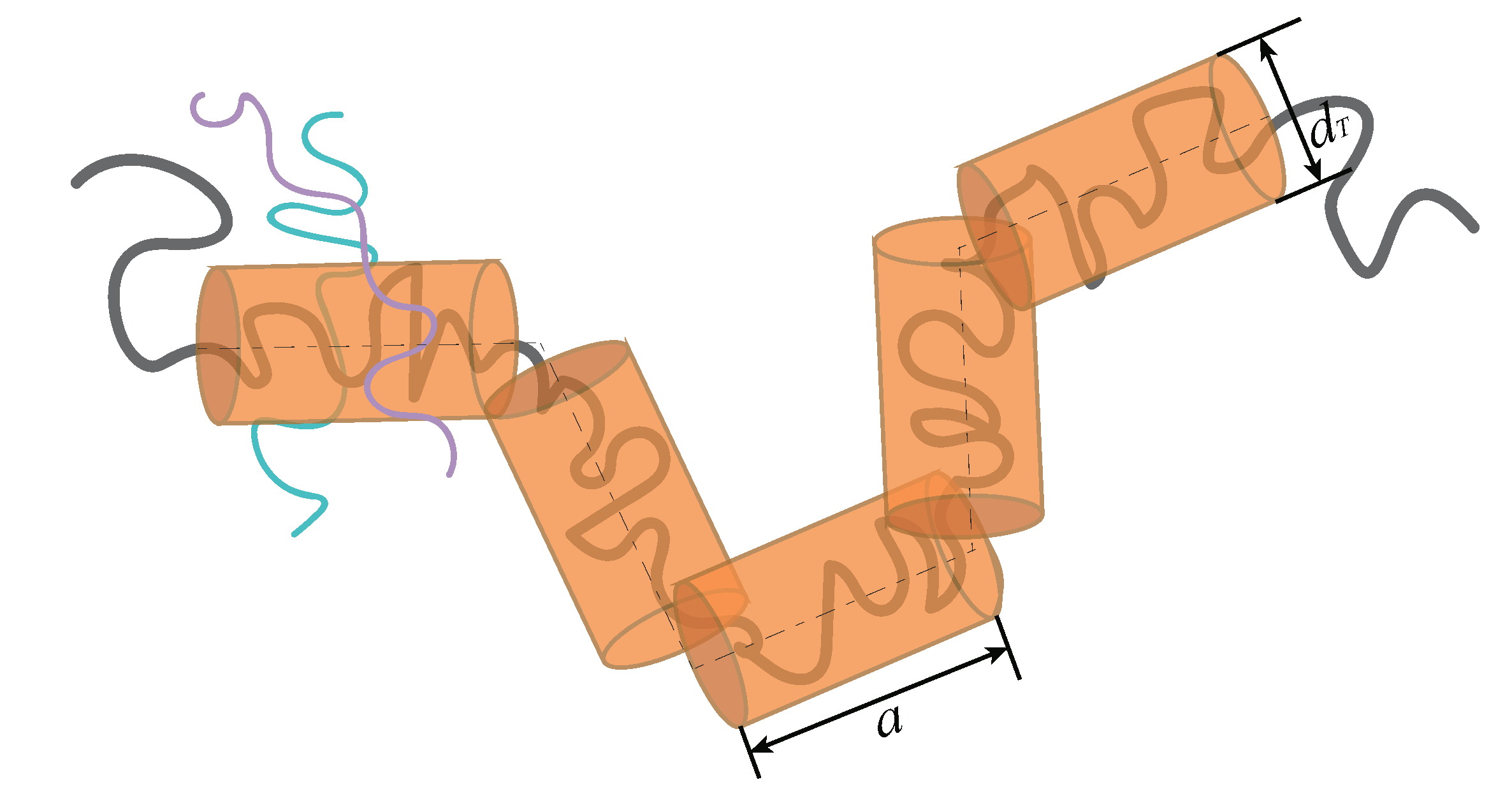
Figure 2.
Monomer mean square displacement of the Kremer–Grest model with from Reference [18]. The black solid lines are the best fits to the slope- regime and the slope- regime. The red asterisk is the intersection of two straight lines, and the red pentagram denotes the time at which the slope of changes from 1/2.

Table 1.
Entanglement parameters for linear polymer melts measured via MSD. For time units, see the original references.
Table 1.
Entanglement parameters for linear polymer melts measured via MSD. For time units, see the original references.
| Ref. | Model or Material | ||||
|---|---|---|---|---|---|
| [24] | KGM | 85 | 2.0 | ||
| [18] | KGM | 33 | 2.0 | ||
| [25] | KGM | 28 | 2.0 | ||
| [26] | KGM | 35 | 2.0 | ||
| [24] | KGM | 34 | 2.0 | ||
| [27] | Polybutadiene K | 21,000 | 72,400 | 2.0 | |
| [28] | Continuous Model | 10,000 | 31,500 | 43 | 2.0 |
| [29] | Coarse–Grained Model | 2.0 |
© 2019 by the author. Licensee MDPI, Basel, Switzerland. This article is an open access article distributed under the terms and conditions of the Creative Commons Attribution (CC BY) license (http://creativecommons.org/licenses/by/4.0/).
Share and Cite
MDPI and ACS Style
Hou, J.-X. Determine Mesh Size through Monomer Mean-Square Displacement. Polymers 2019, 11, 1405. https://doi.org/10.3390/polym11091405
AMA Style
Hou J-X. Determine Mesh Size through Monomer Mean-Square Displacement. Polymers. 2019; 11(9):1405. https://doi.org/10.3390/polym11091405
Chicago/Turabian StyleHou, Ji-Xuan. 2019. "Determine Mesh Size through Monomer Mean-Square Displacement" Polymers 11, no. 9: 1405. https://doi.org/10.3390/polym11091405
Note that from the first issue of 2016, this journal uses article numbers instead of page numbers. See further details here.