
Modelling of Flexible Adhesives in Simple Mechanical States with the Use of the Darijani–Naghdabadi Strain Tensors and Kirchhoff–de Saint-Venant Elastic Potential


Abstract
:
1. Introduction
2. Darijani–Naghdabadi Measures of Strain
- Green–de Saint-Venant strain tensor
- Biot strain tensor
- Hencky strain tensor
- Almansi strain tensor
3. Energy Conjugate Stress Measures for the DN Strain Tensors
- Cauchy stress tensor and linear part of the Almansi–Hamel strain tensor (symmetric part of the spatial displacement gradient)
- Kirchhoff stress tensor and linear part of the Almansi–Hamel strain tensor (symmetric part of the spatial displacement gradient)
- Piola–Kirchhoff stress tensor of the first kind and material deformation gradient
- Piola–Kirchhoff stress tensor of the second kind and Green–de Saint-Venant strain tensor
- Jaumann stress tensor and Biot strain tensor
4. Kirchhoff–de Saint Venant Potential in Description of Flexible Adhesives
5. Force-Stretch Relations
5.1. Simple Tension
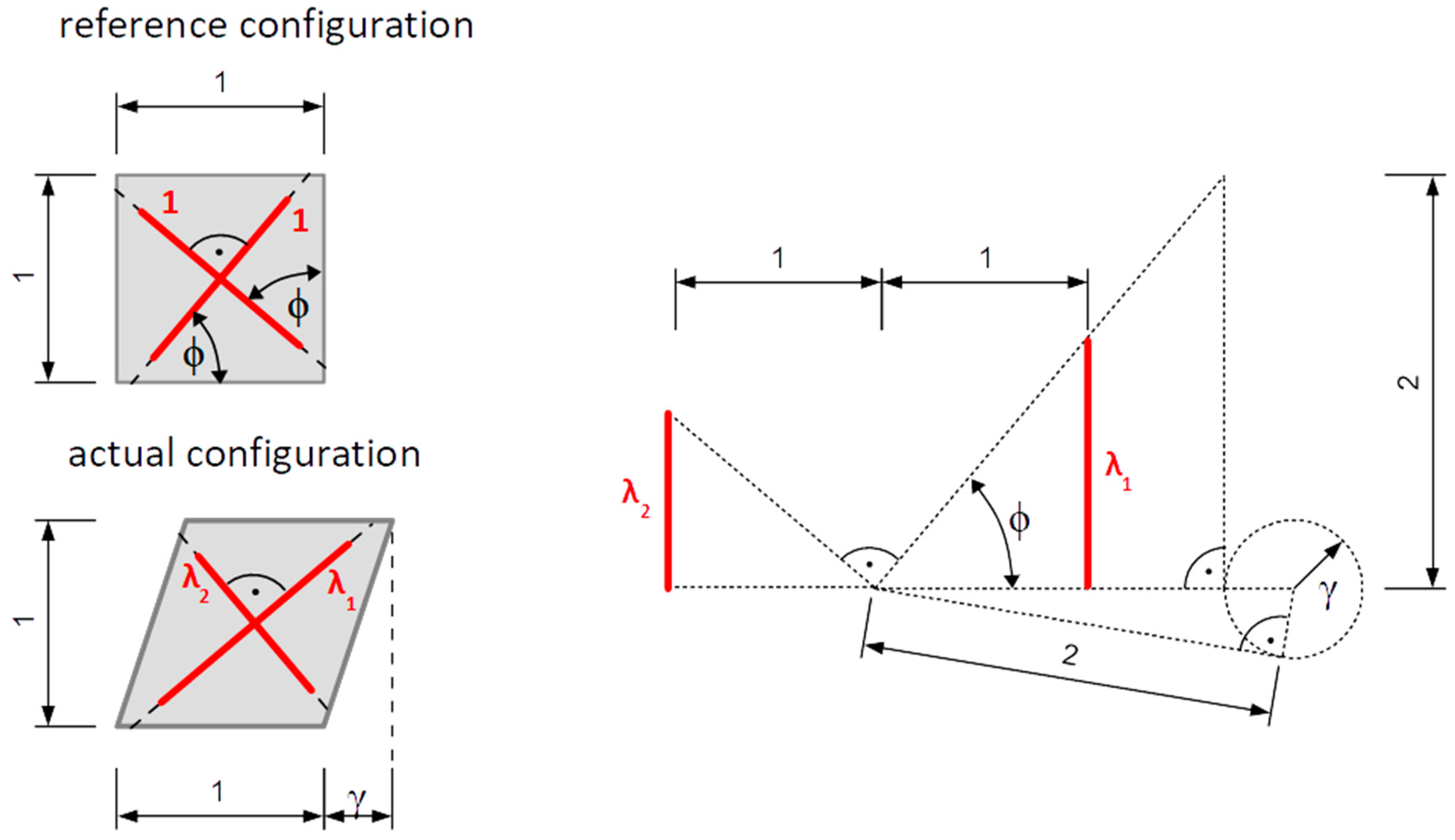
5.2. Simple Shear
6. Released Constraints on Admissible Values of Exponents in a Limit Range of Variation of Stretch
7. Experimental Verification of Proposed Models
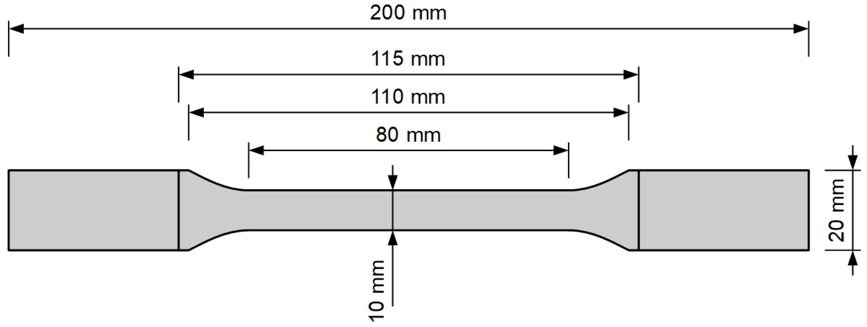
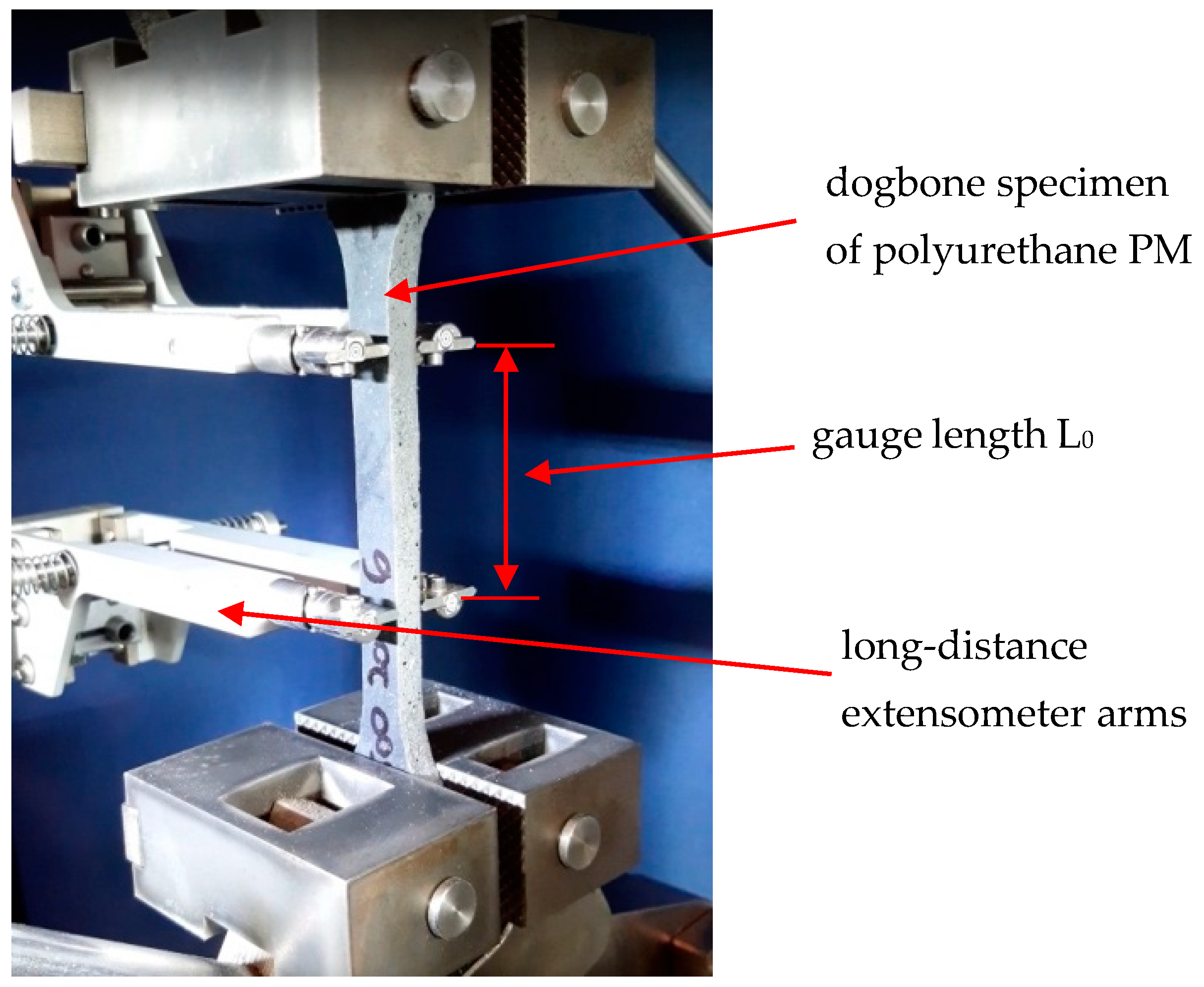
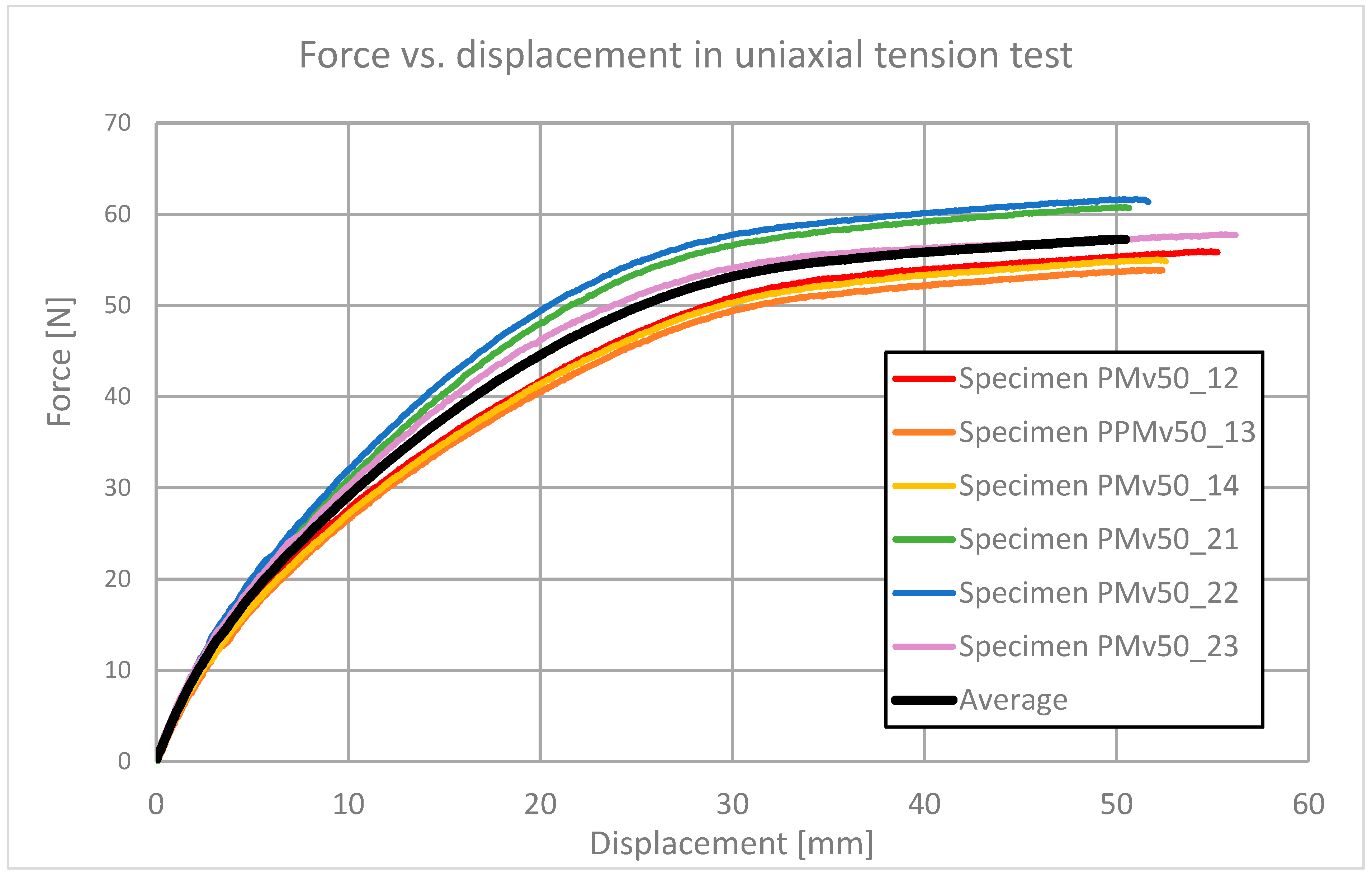
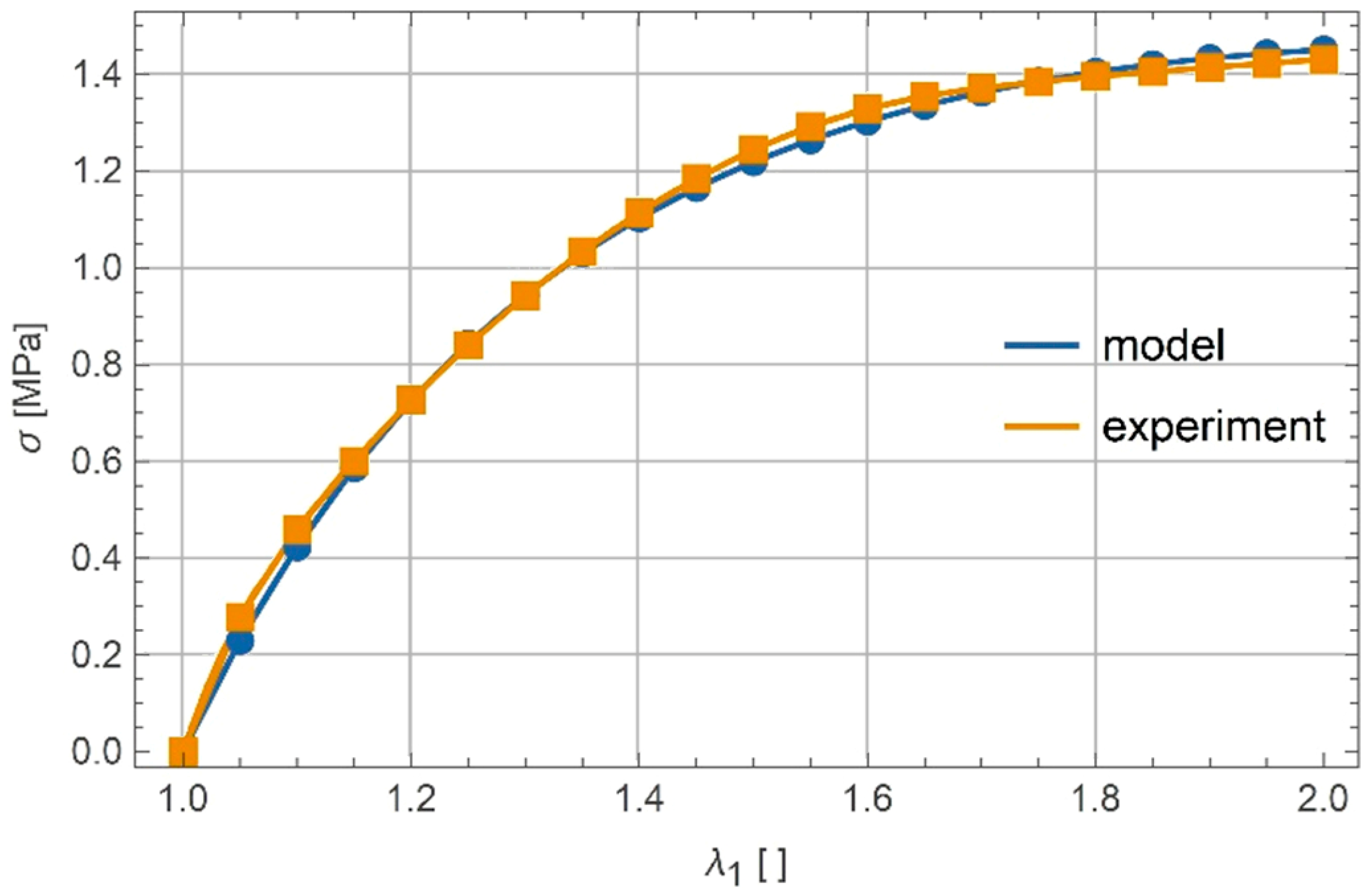
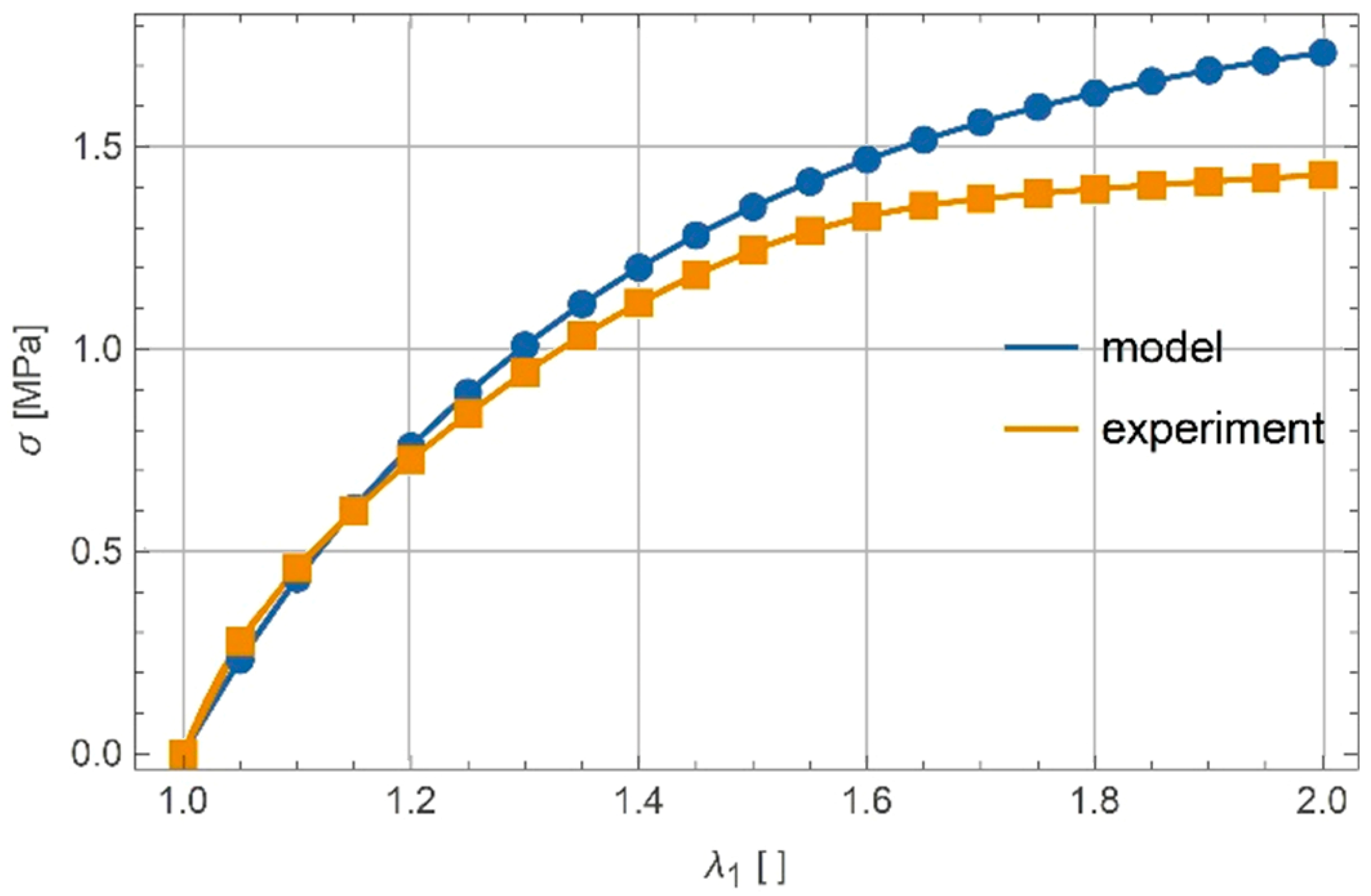
7.1. Uniaxial Tension
Calibration of Parameters and
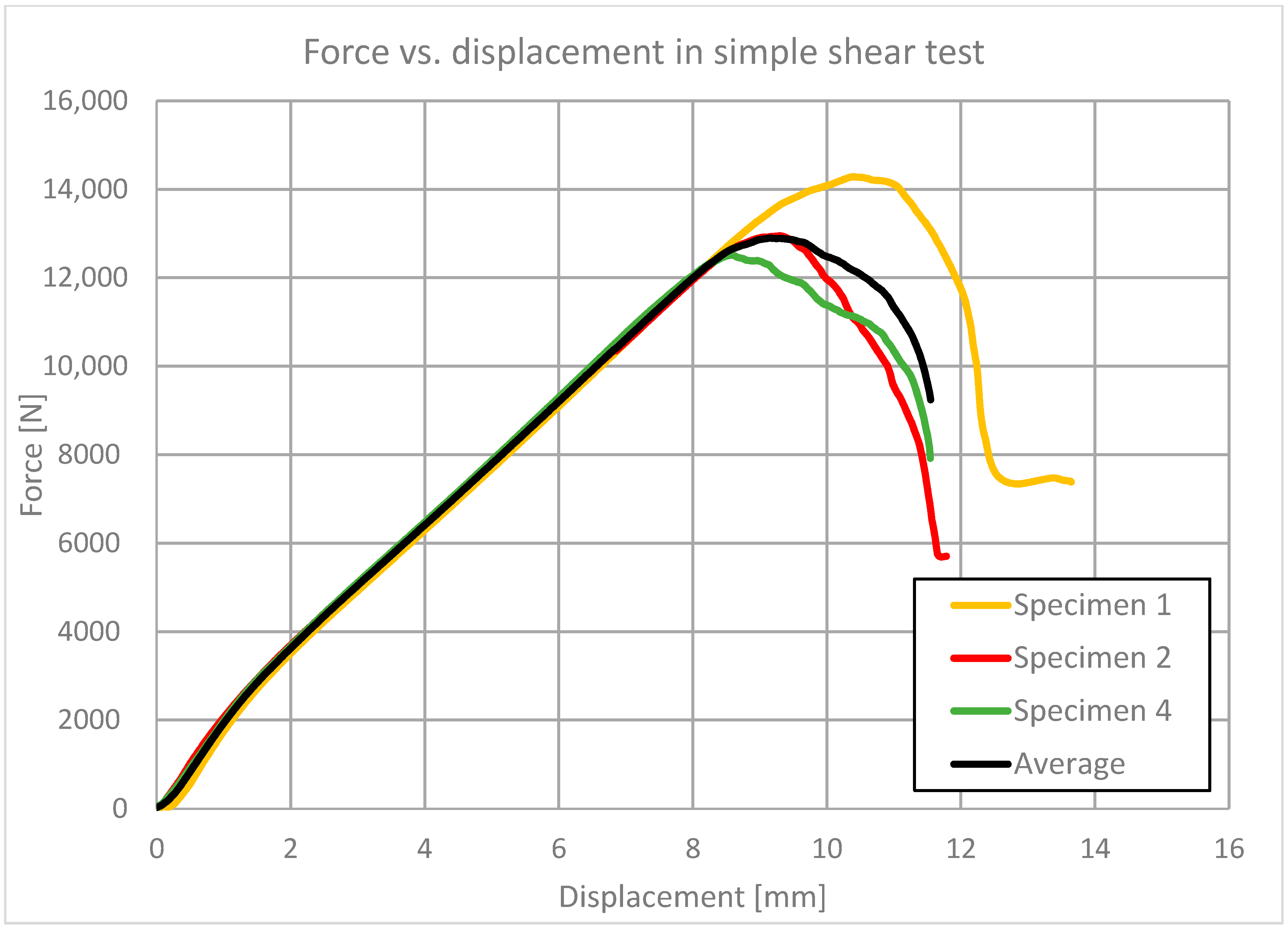
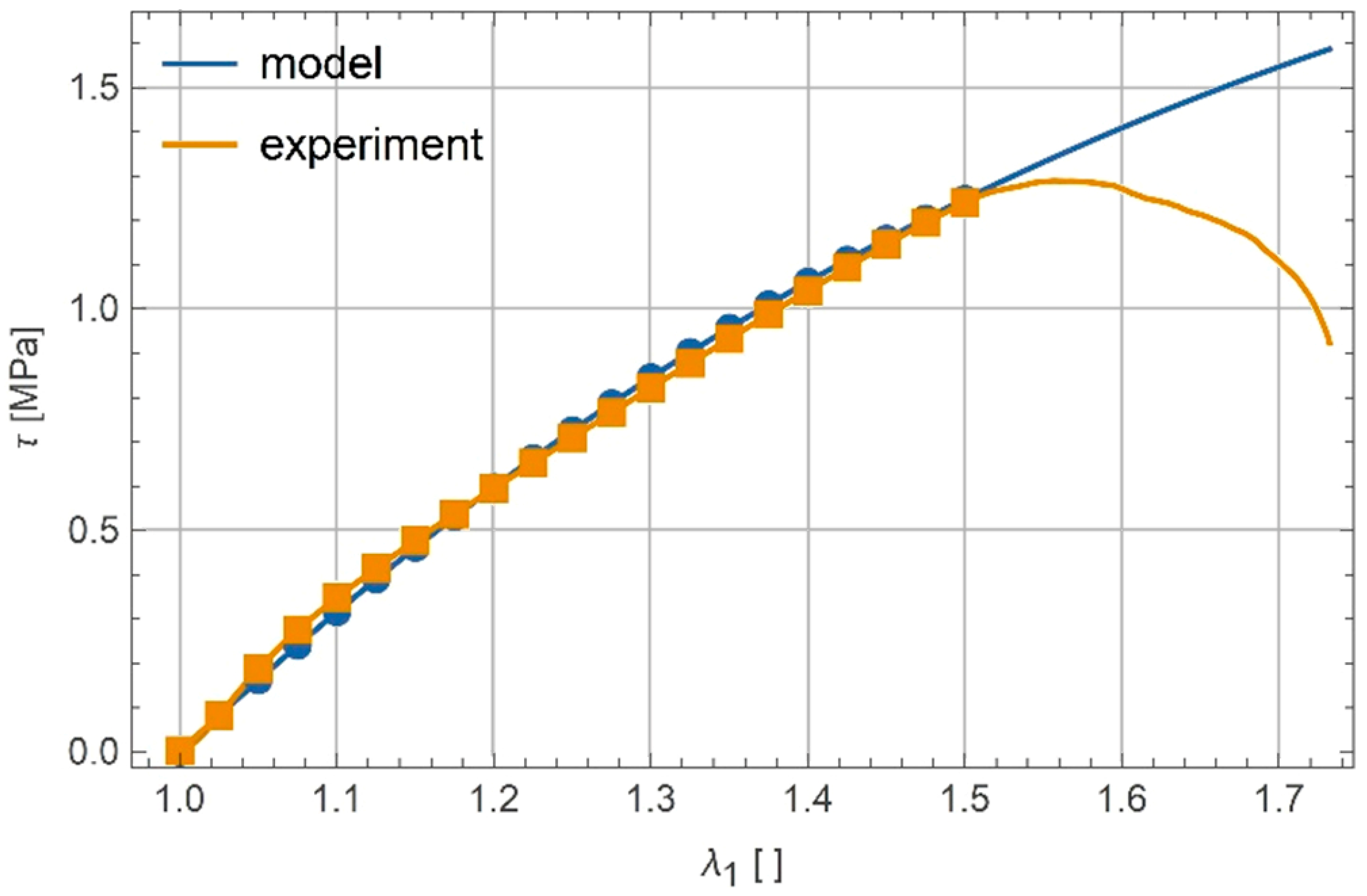
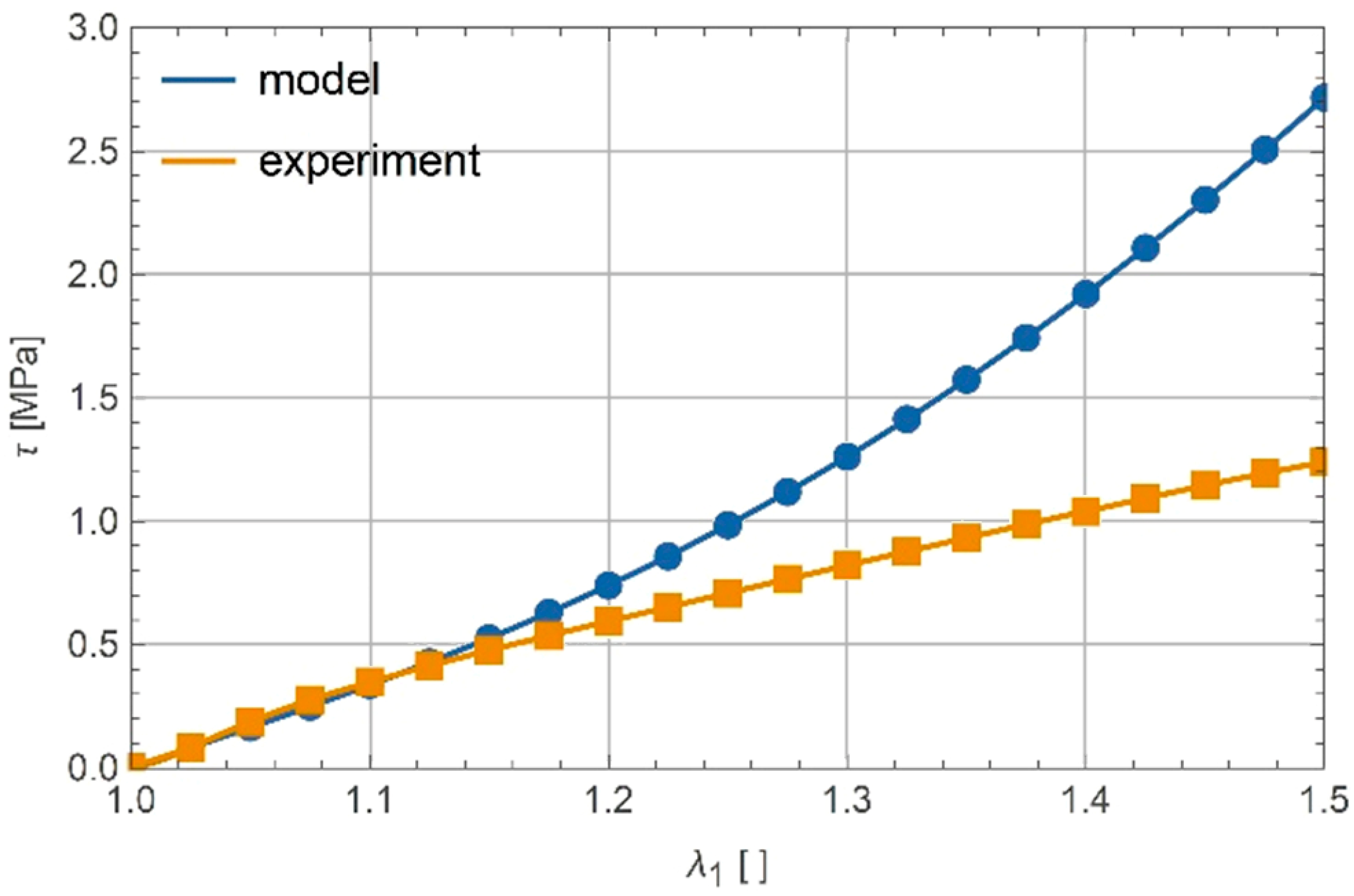
7.2. Shear
Calibration of Parameters and
7.3. Discussion
- The true stress and strain state in the samples differed considerably from what was assumed in the theoretical derivations. This especially concerns the simple shear test in which the stress and strain distribution in the sheared layer is strongly influenced by boundary effects;
- In the case of very large strains, it must be stated that the physical mechanisms of deformation become qualitatively distinct from those which are dominant in the domain of small strain—in particular, breaking the polymer chains becomes more significant. As a result, any approximation of the material’s characteristics with the use of only a single constitutive model—which was assumed to be valid within the whole range of strains—should be expected to fail if the strain becomes sufficiently large;
- The use of the Kirchhoff–de Saint-Venant elastic potential may be inappropriate for the description of the considered material, due to viscous properties of the considered material.
8. Summary and Conclusions
Author Contributions
Funding
Institutional Review Board Statement
Informed Consent Statement
Data Availability Statement
Conflicts of Interest
References
- Kwiecień, A. Strengthening of Masonry using Natural Fibers bonding with highly deformable adhersive. GSTF J. Eng. Technol. 2015, 3. [Google Scholar] [CrossRef]
- Kwiecień, A.; de Felice, G.; Oliveira, D.V.; Zając, B.; Bellini, A.; De Santis, S.; Ghiassi, B.; Lignola, G.P.; Lourenço, P.B.; Mazzotti, C.; et al. Repair of composite-to-masonry bond using flexible matrix. Mater. Struct. Constr. 2016, 49, 2563–2580. [Google Scholar] [CrossRef]
- Seręga, S.; Sena-Cruz, J.; Pereira, E.; Kwiecień, A.; Zając, B. Flexural behaviour of NSM CFRP laminate strip systems in concrete using stiff and flexible adhesives. Compos. Part B Eng. 2020, 195, 1–18. [Google Scholar] [CrossRef]
- Cruz, J.R.; Sena-Cruz, J.; Rezazadeh, M.; Seręga, S.; Pereira, E.; Kwiecień, A.; Zając, B. Bond behaviour of NSM CFRP laminate strip systems in concrete using stiff and flexible adhesives. Compos. Struct. 2020, 245, 1–18. [Google Scholar] [CrossRef]
- Akyıldız, A.T.; Kowalska-Koczwara, A.; Kwiecień, A. Stress distribution in masonry infills connected with stiff and flexible interface. J. Meas. Eng. 2019, 7, 40–46. [Google Scholar] [CrossRef]
- Zając, B.; Kwiecień, A. Thermal compatibility of rigid and flexible adhesives to substrates of historical structures. In Structural Analysis of Historical Constructions: An Interdisciplinary Approach; Springer: Cham, Switzerland, 2019; pp. 1868–1877. ISBN 978-3-319-99440-6. [Google Scholar]
- Kwiecień, A. Shear bond of composites-to-brick applied with highly deformable, in relation to resin epoxy, interface materials. Mater. Struct. Constr. 2014, 47, 2005–2020. [Google Scholar] [CrossRef]
- Rousakis, T.; Ilki, A.; Kwiecień, A.; Viskovic, A.; Gams, M.; Triller, P.; Ghiassi, B.; Benedetti, A.; Rakicevic, Z.; Colla, C.; et al. Deformable polyurethane joints and fibre grids for resilient seismic performance of reinforced concrete frames with orthoblock brick infills. Polymers 2020, 12, 2869. [Google Scholar] [CrossRef] [PubMed]
- Kwiecień, A.; Gams, M.; Rousakis, T.; Viskovic, A.; Korelc, J. Validation of a new hyperviscoelastic model for deformable polymers used for joints between RC frames and masonry infills. Eng. Trans. 2017, 65, 113–121. [Google Scholar]
- Kwiecień, K.; Kwiecień, A.; Stryszewska, T.; Szumera, M.; Dudek, M. Durability of PS-polyurethane dedicated for composite strengthening applications in masonry and concrete structures. Polymers 2020, 12, 2830. [Google Scholar] [CrossRef] [PubMed]
- Szeptyński, P.; Nowak, M. Qualitative analysis of the influence of the non-linear material characteristics of flexible adhesive on the performance of lap joints. Compos. Struct. 2021, 260, 1–11. [Google Scholar] [CrossRef]
- Rivlin, R.S. Large elastic deformations of isotropic materials. IV. Further developments of the general theory. Philos. Trans. R. Soc. Lond. Ser. A Math. Phys. Sci. 1948, 241, 379–397. [Google Scholar]
- Ogden, R.W. Large deformation isotropic elasticity—On the correlation of theory and experiment for incompressible rubberlike solids. Proc. R. Soc. Lond. Ser. A Math. Phys. Sci. 1972, 326, 565–584. [Google Scholar] [CrossRef]
- Yeoh, O.H. Some forms of the strain energy function for rubber. Rubber Chem. Technol. 1993, 66, 754–771. [Google Scholar] [CrossRef]
- Darijani, H.; Naghdabadi, R. Constitutive modeling of solids at finite deformation using a second-order stress-strain relation. Int. J. Eng. Sci. 2010, 48, 223–236. [Google Scholar] [CrossRef]
- Kwiecień, A. Modelowanie równań konstytutywnych polimerów hipersprężystych w złączach podatnych (eng. Modelling of constitutive equations of hyperelastic polymers in flexible joints). In Współczesna Mechanika Konstrukcji w Projektowaniu Inżynierskim; Komitet Inżynierii Lądowej i Wodnej PAN: Warsaw, Poland, 2015; pp. 151–178. ISBN 978-83-938648-6-7. [Google Scholar]
- Kwiecień, A.; Gams, M.; Zając, B. Numerical modelling of flexible polymers. In Proceedings of the 12th International Symposium on Fiber Reinforced Polymers for Reinforced Concrete Structures (FRPRCS-12) & the 5th Asia-Pacific Conference on Fiber Reinforced Polymers in Structures (APFIS-2015) Joint Conference, Nanjing, China, 14–16 December 2015. [Google Scholar]
- Seth, B.R. Generalized Strain Measure with Applications to Physical Problems; MRC Technical Summary Report #248; Armed Services Technical Information Agency: Arlington, VA, USA, 1961. [Google Scholar]
- Hill, R. On constitutive inequalities for simple materials—I. J. Mech. Phys. Solids 1968, 16, 229–242. [Google Scholar] [CrossRef]
- Farahani, K.; Naghdabadi, R. Basis free relations for the conjugate stresses of the strains based on the right stretch tensor. Int. J. Solids Struct. 2003, 40, 5887–5900. [Google Scholar] [CrossRef]
- Tsai, M.Y.; Oplinger, D.W.; Morton, J. Improved theoretical solutions for adhesive lap joints. Int. J. Solids Struct. 1998, 35, 1163–1185. [Google Scholar] [CrossRef]
- Kisiel, P. Model Approach for Polymer Flexible Joints in Precast Elements Joints of Concrete Pavements. Ph.D. Thesis, Cracow University of Technology, Kraków, Poland, 2018. [Google Scholar]
- Mathematica; Version 12.2 2020; Wolfram Research, Inc.: Champaign, IL, USA, 2020.
Publisher’s Note: MDPI stays neutral with regard to jurisdictional claims in published maps and institutional affiliations. |
© 2021 by the authors. Licensee MDPI, Basel, Switzerland. This article is an open access article distributed under the terms and conditions of the Creative Commons Attribution (CC BY) license (https://creativecommons.org/licenses/by/4.0/).
Share and Cite
Szeptyński, P.; Gams, M.; Kwiecień, A. Modelling of Flexible Adhesives in Simple Mechanical States with the Use of the Darijani–Naghdabadi Strain Tensors and Kirchhoff–de Saint-Venant Elastic Potential. Polymers 2021, 13, 1639. https://doi.org/10.3390/polym13101639
Szeptyński P, Gams M, Kwiecień A. Modelling of Flexible Adhesives in Simple Mechanical States with the Use of the Darijani–Naghdabadi Strain Tensors and Kirchhoff–de Saint-Venant Elastic Potential. Polymers. 2021; 13(10):1639. https://doi.org/10.3390/polym13101639
Chicago/Turabian StyleSzeptyński, Paweł, Matija Gams, and Arkadiusz Kwiecień. 2021. "Modelling of Flexible Adhesives in Simple Mechanical States with the Use of the Darijani–Naghdabadi Strain Tensors and Kirchhoff–de Saint-Venant Elastic Potential" Polymers 13, no. 10: 1639. https://doi.org/10.3390/polym13101639