Nonlinear Progressive Damage Analysis of Notched or Bolted Fibre-Reinforced Polymer (FRP) Laminates Based on a Three-Dimensional Strain Failure Criterion

Abstract

Notching and bolting are commonly utilised in connecting fibre-reinforced polymer (FRP) laminates. These mechanical methods are usually superior to other connections, particularly when joining thick composite laminates. Stress distributions, damage modes and ultimate strengths in notched or bolted FRP laminate designs are of particular interest to the industrial community. To predict the ultimate strengths and the failure processes of notched or bolted composite laminates, nonlinear progressive damage analyses (PDA) based on the finite element method (FEM) at the meso-scale level are performed in this paper. A three-dimensional strength criterion in terms of strains, which can distinguish different damage modes, was developed and adopted in the analysis model to detect damage initiation in the laminates. Different material degradation methods and the influence of cohesive layers were discussed and compared with results of verification experiments. The results showed that the analysis model that used the succinct strength criterion proposed in this paper could properly predict the damage initiation and the ultimate strengths of notched or bolted FRP laminates. The errors between the numerical results and experimental data were small. The material degradation method with continuum damage mechanics (CDM)-based exponential damage factors using the damage index as the independent variable achieved greater accuracy and convergence than the method with CDM-based exponential damage factors using the square index as the independent variable or than the method with constant damage factors. Adding cohesive layers in the model had negligible influence on the final results, largely because the succinct analysis model proposed in this paper is sufficiently accurate in cases of small delamination.

1. Introduction

Fibre-reinforced polymers (FRPs) are composed of high-strength fibres embedded in a polymer matrix. They were first used in military applications approximately 50 years ago [1]. Because of their advantageous properties, including high specific strength, corrosion resistance and fatigue resistance, FRP products such as laminates have emerged as useful materials for numerous applications in the aerospace, automotive and construction industries.

Connections involving FRP laminate structures will inevitably occur in application. There are three main types of connections: bolting, bonding and clamping [2]. Among them, bolting is usually superior compared with other connections, particularly for thick FRP laminates. However, bolted connections require the FRP laminates to be circularly notched, which can cause serious stress concentrations. Moreover, the large local pressure from the bolt during loading is problematic for FRP laminates. These two disadvantages may greatly influence the strength of the bolted connection and may be potential sources of safety hazards in applications involving FRP structures. Therefore, investigating the failure characteristics of notched or bolted FRP laminates and finding feasible methods to predict the ultimate strengths of these components are of high interest.

Although research regarding the failure behaviours and strengths in FRP laminates has existed worldwide for decades, there remains no method that can perfectly predict the failure characteristics of FRP laminates, particularly in complex cases [3,4]. In the early stages of this research topic, Whitney and Nuismer [5] established the point stress criterion (PSC) and average stress criterion (ASC) to predict the strength of notched FRP laminate. Karlak [6] proposed the modified PSC based on research from Whitney and Nuismer. Pipes [7] discussed the influence of stress concentrations on the strength of notched FRP laminate. Based on a large number of failure experiments of FRP single ply, many strength criteria for unidirectional orthotropic plates were proposed to predict the strengths of the FRP laminates, such as the Hankinson criterion, the Strussi criterion, the Norris–Fischer criterion, the Kopnov criterion etc. [8]. Among them, some strength criteria were presented in the form of quadratic polynomials, such as the Hill–Tsai criterion, the Hoffman criterion and the Tsai–Wu criterion. These are commonly used today, mainly because of their simple forms and relatively good accuracy [9]. The Hashin criterion [10] and the Puck criterion [11], which can apply different criteria according to different damage modes, are also widely used in the present design of FRP laminates. The methods mentioned above can usually only predict the damage initiation of the FRP laminates, rather than considering the failure process and final strength. Chang was the first to propose a two-dimensional model based on progressive damage analysis (PDA) in the frame of finite element method (FEM) to simulate the failure processes of FRP laminates and to predict their ultimate strengths [12,13]. Tan further developed Chang’s method and discussed the range of choices of degradation factors [14,15]. Camanho [16], Shokrieh [17,18] and Tserpes [19] established a three-dimensional FEM model to perform PDA on the laminates that decreased the material stiffness according to the different damage modes. Most of the above progressive damage analyses used constant values for material degradation factors, which can also be called damage factors. They were determined experimentally or defined empirically. Lapczyk [20] established a two-dimensional progressive damage model of FRP laminates adopting the continuum damage mechanics (CDM)-based linear material degradation factors. Linde [21] proposed a three-dimensional model with CDM-based exponential damage factors that used the square index as the key independent variable. This predicted the failure process and the ultimate strength of the fibre metal laminate (FML). Frizzell and McCarthy [22] described a three-dimensional damage finite element model that was used to simulate the damage evolution of FML joints. Damage regularisation was implemented in this model to mitigate the mesh dependency. Cohesive zones or cohesive layers, whose basic concept was proposed by Dugdale [23] and Barenblatt [24], are now increasingly used to model delamination damage in FRP laminates. Needleman [25,26] established a cohesive model according to the traction–separation law. Camanho [27] proposed a cohesive element based on truss-like mixed-mode cohesive laws, which are widely used and implemented in the commercial finite element code ABAQUS [28]. Goutianos and Sorensen [29] proved that the truss-like mixed-mode cohesive laws are path dependent. McGarry and Mairtin et al. [30,31] performed a thorough analysis of potential-based and non-potential-based cohesive zone models under conditions of mixed-mode separation and mixed-mode over-closure. Admittedly, incorporating cohesive layers into the analysis model can usually improve the accuracy of numerical calculations, particularly in cases of serious delamination damage. However, blindly adding the cohesive layers will increase the modelling difficulty and waste computing resources. The literature has shown that an analysis model with three-dimensional failure laws can effectively simulate delamination and accurately predict the ultimate laminate strength, particularly in situations of in-plane loading where delamination is relatively small [16,17,18,32,33].

Based on previous studies, the three-dimensional finite element progressive damage analyses for notched or bolted FRP laminates were performed in this paper. A three-dimensional strain strength criterion, similar to that described by Linde [21], was proposed and used in the analysis model to predict damage initiation according to different damage modes. After damage occurred, the material stiffness matrix was degraded by the damage tensor, which was strictly derived from the theory of damage mechanics. The damage factors constituted the damage tensor. An exponential form of the damage factors was proposed in this paper and compared with the similar exponential form that used the square index as the independent variable and with a conventional constant form for the damage factors. This exponential form was determined on the basis of continuum damage mechanics and adopted the damage index suggested by Tsai [34] as the key independent variable. The influence that the presence or absence of cohesive layers had on the model was also investigated through a case study. The numerical results were verified by corresponding experiments.

2. Progressive Damage Analysis Methodology

2.1. Progressive Damage Analysis Procedure

Damage mechanics (DM) forms the theoretical foundation of progressive damage analysis on solid materials [35]. The basic assumption of this analysis is that the material can still bear the load after the damage occurs. It includes three main points: the material strength criterion, the damaged material constitutive relation and the stress strain field solution. The procedure of the progressive damage analysis is illustrated in Figure 1.

Figure 1. Main progressive damage analysis procedure.

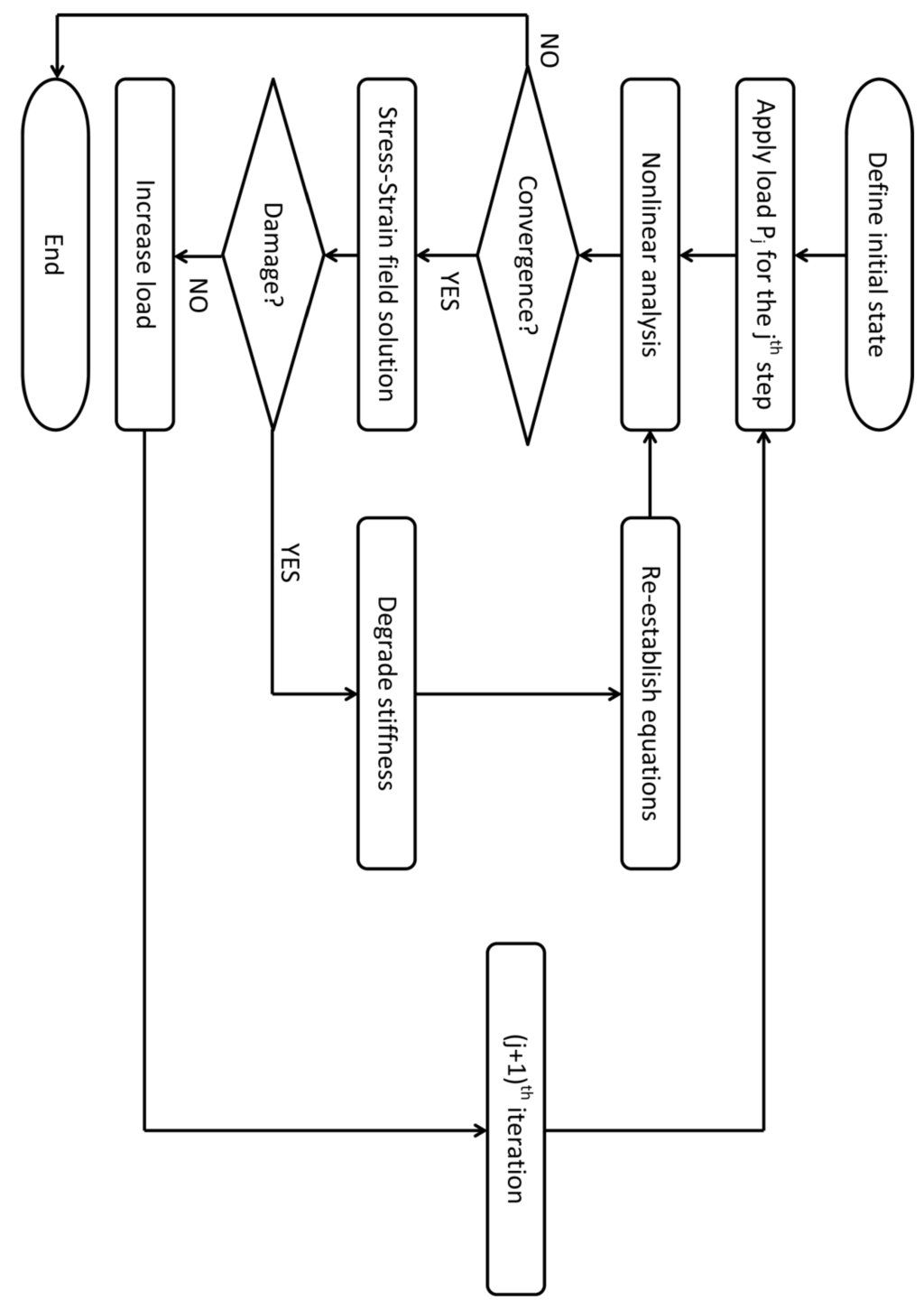
Figure 1. Main progressive damage analysis procedure.

2.2. Material Strength Criterion

A succinct three-dimensional strain strength criterion was developed and used in the progressive damage analysis model. This strength criterion is based on research from Linde [21] and is extended from two dimensions to three dimensions. It can predict three modes of composite damage: fibre damage, matrix damage and delamination damage. The criterion inequalities are listed in Table 1 according to different damage modes.

Table 1. Inequalities of the strength criterion according to different damage modes.

Damage mode	Graphic representation	Strength criterion inequality
Fibre damage
Matrix damage
Delamination damage

Table 1. Inequalities of the strength criterion according to different damage modes.

Damage mode	Graphic representation	Strength criterion inequality
Fibre damage
Matrix damage
Delamination damage

As shown in Table 1, the ε_ij (i,j = 1,2,3) represent the components of strain in the corresponding directions. The ε_ij terms that use superscripts represent the related strain limits. The superscripts (t,c,s) stand for tension, compression and shear, respectively. If the term on the left side of any of the three inequalities is greater than or equal to one, the corresponding damage will occur.

In this strength criterion, strain is used to evaluate the damage. Compared with other stress-based criteria, this can facilitate the nonlinear iteration calculations because most nonlinear mechanics calculations apply the strain increment for iteration [36]. Furthermore, this strength criterion can distinguish between damage modes. This makes it possible to decrease the material stiffness taking the different damage modes into account. The inequalities of the criterion include both linear terms and quadratic terms and also combine the tension and compression effects into a single inequality, which makes the strength criterion accurate and concise.

2.3. Constitutive Relation for Damaged Orthotropic Material

According to the assumption of the progressive damage analysis, material damage can be held equivalent to the degradation of corresponding material properties [35]. The degradation methods used can be classified into two main categories: directly reducing the elastic constants, namely Young’s modulus and Poisson’s ratio, and reducing the values of terms in the stiffness matrix. Chang [12] initially proposed the first method, which remains in use [20]. However, previous research has shown that this method may cause convergence problems in finite element calculations, mainly because inappropriate reduction factors will lead to a singular stiffness matrix [37]. The second method, which reduces the values of terms in the stiffness matrix, was adopted in this paper to degrade the properties of the damaged material.

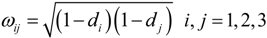
To establish the constitutive relation in the damaged orthotropic material, the damage tensor M (ω), consisting of damage factors d_i, was derived based on the theory of damage mechanics and introduced into the numerical model. In a physical sense, the damage factors d_i (i = 1,2,3) represent the reduction ratio of effective bearing area perpendicular to the three principle directions of the material [38]. This also corresponds to the three damage modes mentioned in Section 2.2. The selection of damage factors is discussed in detail in Section 3.2.

In the three-dimensional case, the damage tensor M (ω), which is a second-order tensor related to d_i, can be defined as:

(1)

with

(2)

Introducing the concept of effective stress and apparent stress σ results in

(3)

where and σ are first-order tensors containing six stress components.

The complementary energy W for the undamaged material is defined as:

(4)

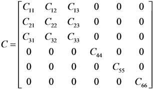
where C is the stiffness matrix of the undamaged orthotropic material (C⁻¹ is the compliance matrix), which can be written as:

(5)

Based on the assumption of energy equivalence, that is, the form of the complementary energy of the damaged material, W_d is identical to that of the undamaged material W, and the following can be derived:

(6)

Substituting (3) into (6) results in:

(7)

Comparing (4) and (7) gives:

(8)

Therefore, the stiffness matrix of the damaged material is:

C_d = M⁻¹ : C : M^−T

(9)

Finally, at the damaged material points, the constitutive model expressed in terms of stress-strain relation can be written as:

σ = C_d : ε

(10)

2.4. Method for Solving Stress

Because the analytical stress solution is usually difficult to obtain, numerical methods are commonly used to solve the stress field [39]. These include the finite difference method, the finite element method, the boundary element method, etc. In this paper, the finite element method (FEM) was adopted. A three-dimensional FEM model was established in the general FEM software ABAQUS. The material progressive damage model was implemented using the ABAQUS subroutine UMAT [28]. In case study 2, which represents bolted CFRP laminate under unidirectional tension, the cohesive layers used were composed of the ABAQUS built-in cohesive elements [28].

3. Case Study 1: Notched FRP Laminate under Unidirectional Tension

3.1. Geometry and Material Properties

The specimen studied in case study 1 was a glass fibre-reinforced polymer (GFRP) laminate containing a central hole. Its diagrammatic sketch and geometry information are shown in Figure 2.

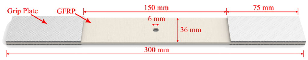
Figure 2. Diagrammatic sketch and geometry of the GFRP laminate specimen.

Figure 2. Diagrammatic sketch and geometry of the GFRP laminate specimen.

The fibre was S2 glass fibre and the polymer was epoxy-based resin. The property data of the specimen came from O’Higgins [40] and is listed in Table 2.

Table 2. Material properties of the specimen (each ply).

Elastic property	Value	Strength property *	Value
E1	52,000 MPa		1,840 MPa
E2 = E3	8,000 MPa		1,580 MPa
G12= G13	3,000 MPa		44 MPa
G23	2,900 MPa		172 MPa
v12 = v13	0.28	S12= S13	39 MPa
v23	0.34	S23	32 MPa

Note: * the strain limits ε_ij are equal to s_ij / c_ij (i = 1,2,3).

Table 2. Material properties of the specimen (each ply).

Elastic property	Value	Strength property *	Value
E1	52,000 MPa		1,840 MPa
E2 = E3	8,000 MPa		1,580 MPa
G12= G13	3,000 MPa		44 MPa
G23	2,900 MPa		172 MPa
v12 = v13	0.28	S12= S13	39 MPa
v23	0.34	S23	32 MPa

Note: * the strain limits ε_ij are equal to s_ij / c_ij (i = 1,2,3).

This specimen was a quasi-isotropic laminate with the stacking sequence [45 / 0 / −45/ 90]_2s, containing four [45 / 0 / −45/ 90] sub-laminates. The thickness of each ply was 0.2 mm, meaning that the total laminate thickness was 3.2 mm. The tensile load was along the X-axis, which was the direction of the 0° ply (Figure 3). The schematic of the calculation model that includes the fibre orientation coordinate and load and boundary conditions is shown in Figure 3.

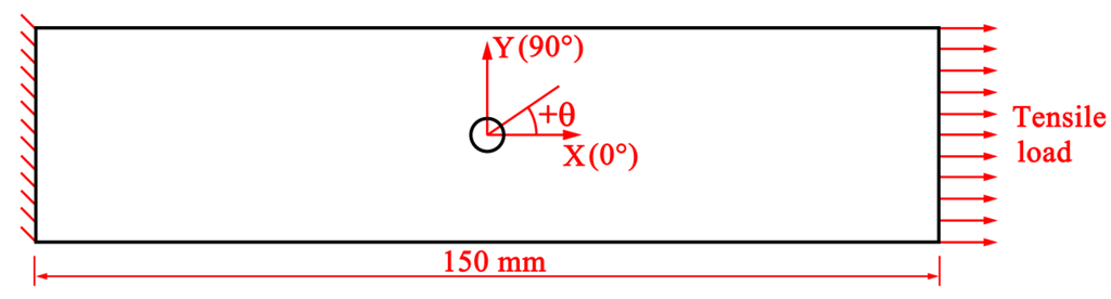
Figure 3. Schematic of the simplified calculation model with the fibre orientation coordinate, load conditions and boundary conditions.

Figure 3. Schematic of the simplified calculation model with the fibre orientation coordinate, load conditions and boundary conditions.

3.2. Finite Element Model

Based on the above simplified calculation model, the FE model was established in the general FEM software ABAQUS. The three-dimensional solid element C3D8 was adopted, which is an 8-node linear brick [28]. Because stress was concentrated near the circular notch, the mesh in the stress concentration zone was refined. Furthermore, because of the stacking symmetry, only half of the specimen was modelled (Figure 4).

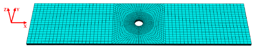
Figure 4. Finite element model of the GFRP laminate specimen with the global coordinate system.

Figure 4. Finite element model of the GFRP laminate specimen with the global coordinate system.

3.3. Selection of the Damage Factors

After establishing the material constitutive relation and the finite element model, the damage factors in the damage tensor were determined so as to carry out the degradation of the damaged material. The commonly used forms of the damage factor are classified into two categories: the constant form and the continuum damage mechanics (CDM)-based variable form. The latter can also be divided into two classes: the linear form and the exponential form. In this paper, constant damage factors and two types of CDM-based exponential damage factors were adopted in calculations and compared for accuracy and convergence.

3.3.1. Constant Damage Factors

As the name implies, the constant damage factors d_i are set to constant values, which are usually positive decimals slightly smaller than one. They are widely used mainly for their simplicity and convenience. The specific values of d_i (i = 1,2,3) in this paper according to related damage modes are listed in Table 3. These values were empirically determined.

Table 3. Specific values of corresponding damage factors.

Damage mode	Damage factor	Value
Fibre damage	d1	0.99
Matrix damage	d2	0.95
Delamination damage	d3	0.95

Table 3. Specific values of corresponding damage factors.

Damage mode	Damage factor	Value
Fibre damage	d1	0.99
Matrix damage	d2	0.95
Delamination damage	d3	0.95

3.3.2. Two Types of CDM-Based Exponential Damage Factors

In contrast with the constant damage factors, the variable damage factors can change with increasing damage. They are based on the theory of continuum damage mechanics and their values are directly related to the damage degree. Therefore, it is important to evaluate the damage degree. According to the damage mechanics, the damage degree relates to the external load and is positively correlated with the ratio between the applied stress (or strain) and the material strength [34]. To quantify the damage degree, the damage index k, defined as the ratio between the applied stress (or strain) and the ultimate strength, was introduced [32]. For the strength criterion proposed in this paper, the terms on the left side of the strength inequalities can be written in the tensor form [34]:

G_ijε_iε_j + G_iε_i

(11)

Letting every ε reach its ultimate value when:

(12)

Substituting for results in:

(13)

Solving the quadratic equation, where a = G_ijε_iε_j, b = G_iε_i and :

ax² + bx − 1 = 0

(14)

Getting the positive quadratic root:

(15)

Therefore:

(16)

With a clear physical concept, the damage index k is a good coefficient to use when evaluating the degree of damage. However, in some reports [21,41], the square index f was adopted to evaluate the damage. Its definition is

(17)

Tsai [34] pointed out that the failure analysis of composite materials should be based on k, not f. Unlike the damage index k, the square index f does not have any physical meaning and is not associated with the ratio between the applied stress (or strain) and the ultimate strength. The envelope curve of the strength criterion like G_ijε_iε_j + G_iε_i ≥ 1 is an ellipse that is not centred at the origin, because the linear term exists and the tensile and compressive strengths are different. In Figure 5, the differences between the envelopes for k and f are presented, when both of them are equal to 1.5.

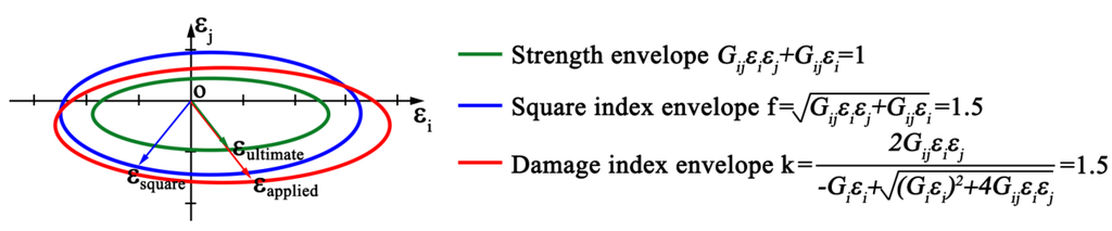
Figure 5. Comparison between the damage index k envelope and the square index f envelope.

Figure 5. Comparison between the damage index k envelope and the square index f envelope.

As shown in Figure 5, the damage index envelope with k = 1.5 expands from the strength envelope like rays radiating from the origin, whereas the square index envelope is only the confocal ellipse of the strength envelope with increasing size. When k is equal to 1.5, it is immediately known that ε_applied / ε_ultimate = 1.5, which is directly related to the damage degree. However, a square index of 1.5 only implies that the material is damaged qualitatively. It is not related to the damage degree in any quantitative way. Furthermore, the figure shows that the square index f will underestimate the damage degree in some cases, and overestimate it in others.

Based on the above analysis, the damage index k was adopted in this paper to construct the damage factor as a key independent variable. The degree of damage in each principle direction was expressed by the corresponding damage index k. Based on the specific strength criterion and the derivation from (12) to (16), k_i (i = 1,2,3) can be written as:

(18)

(19)

(20)

Assuming that the damage evolution was also controlled by the fracture energy dissipated during material damage [21] and introducing the equivalent displacement into the model to alleviate the mesh dependency because of the strain-softening behaviour [20], the three damage factors d_i (i = 1,2,3) can be expressed as:

(21)

(22)

(23)

In the above equations, δ_ij (i, j = 1,2,3) are the equivalent displacements, and δ_ij = ε_ij × L_c, where L_c is the characteristic length. W_i (i = 1,2,3) represent the dissipated energies of the related failure modes.

Despite the lack of theoretical basis and being evaluated by Tsai as a bad index to use for composite materials, the square index f was still adopted to construct the damage factor, but only for comparison purposes. Based on the specific strength criterion and (17), f_i (i = 1,2,3) can be written as:

(24)

(25)

(26)

Substituting f instead of k into (17), (18) and (19), the CDM-based exponential damage factors using the square index as the key independent variable can be written as:

(27)

(28)

(29)

3.4. Comparison of Numerical and Experimental Results

The experimental data for verification came from O’Higgins [40]. First, the stress-strain curves and the open hole tension (OHT) strengths are shown and compared in Figure 6 and Table 4. According to ASTM Standard D5766/ D5766M-02, the stress is the axial average stress (equal to the load divided by the gross cross-sectional area), and the strain is the axial average strain. The OHT strength is defined as the ultimate tensile load divided by the gross cross-sectional area [42].

Figure 6. Experimental versus three numerical stress-strain responses.

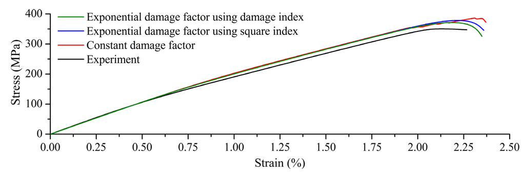
Figure 6. Experimental versus three numerical stress-strain responses.

Table 4. Comparison of OHT strengths from numerical and experimental results.

Damage factor	Numerical result	Experimental result	Error
Constant	385.23 MPa	350 MPa	10.07%
Exponential (square index)	376.94 MPa		7.70%
Exponential (damage index)	370.60 MPa		5.89%

Table 4. Comparison of OHT strengths from numerical and experimental results.

Damage factor	Numerical result	Experimental result	Error
Constant	385.23 MPa	350 MPa	10.07%
Exponential (square index)	376.94 MPa		7.70%
Exponential (damage index)	370.60 MPa		5.89%

Figure 6 shows that the three numerical result curves generally coincide with the experimental result curve. The OHT strengths are shown in Table 4. The numerical result adopting the CDM-based exponential damage factors, which used the damage index as the independent variable, shows least variation from the experimental data in the three numerical results.

Compared with the degradation method using constant damage factors, the method with the exponential damage factors using the damage index as the independent variable achieved higher accuracy and a smoother stress-strain curve, along with a considerably shorter iteration convergence time. When compared with adopting similar exponential damage factors but using the square index as the independent variable, adopting the exponential damage factors with the damage index yielded a more accurate result in addition to a clear physical meaning.

Because the numerical results from the three degradation methods were similar, and because the method with exponential damage factors that used the damage index generated results closer to the experimental outcomes, all of the following shown numerical simulations are based on this method.

The deformation and damage diagram of the specimen in the final failure state, which is defined as the termination of the numerical calculation, is shown in Figure 7, wherein the red zones indicate the damaged zones and the blue zones indicate no damage.

Figure 7. Deformation and damage distribution at the specimen in the final failure state with the fibre orientation coordinate.

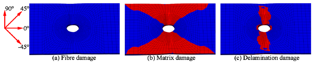
Figure 7. Deformation and damage distribution at the specimen in the final failure state with the fibre orientation coordinate.

As shown in Figure 7, all three types of damage existed at or near the circular notch. In the final failure state, the tensile fracture occurred at the cross-sections near the notch, as evidenced by apparent necking in this region.

The fibre, matrix and delamination damage evolutions at the laminate specimen are shown in Figure 8, Figure 9 and Figure 10, respectively. Because the damage evolutions in the two modelled sub-laminates were similar, only the damage diagrams of the four plies of the second sub-laminate (counting from outside to inside) are illustrated with the fibre orientation coordinate. Each of the following figures shows damage evolution at the different plies of the sub-laminate in three loading states: the damage initiation state, the bearing capacity limit state and the final failure state. As the name implies, in the damage initiation state, the corresponding damage starts to occur; in the bearing capacity limit state, the bearing capacity of the specimen reaches the maximum value; in the final failure state, the specimen reaches its ultimate failure state and the numerical calculation simultaneously terminates.

Figure 8 shows that the fibre damage first occurred at the notch edge of the 0° ply at a stress of 348.08 MPa. Subsequently, damage at the 0° ply extended from the notch to the sides, and some areas near the notches of both the 45° and −45° plies started getting damaged. After the tensile bearing capacity of 370.60 MPa was reached, the damage in the 45°, 0° and −45° plies extended quickly along the Y-axis. This resulted in penetrating damage zones and caused the final failure of the laminate. In the failure process of the laminate, no fibre damage was observed at the 90° ply. The damage area of the 0° ply was always larger than those of the 45° and −45° plies under the same load.

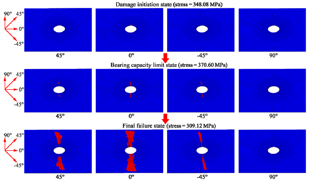
Figure 8. Illustration of fibre damage evolution at four plies of the second sub-laminate in different loading states.

Figure 8. Illustration of fibre damage evolution at four plies of the second sub-laminate in different loading states.

Figure 9. Illustration of matrix damage evolution at four plies of the second sub-laminate in different loading states.

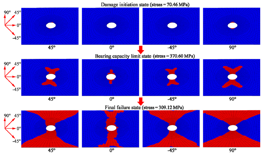
Figure 9. Illustration of matrix damage evolution at four plies of the second sub-laminate in different loading states.

Figure 9 shows the damage evolution of the matrix. The damage was initiated at the notch edge of the 90° ply under an average tensile stress of 70.46 MPa. It also occurred shortly thereafter at the notches in the 45° and −45° plies. Following this, the matrix damage at the 45°, −45° and 90° plies spread in a butterfly-like shape from the circular notch to the ply sides. The damage in the 0° ply appeared much later than that in the 45°, −45° and 90° plies. It first occurred at the notch edge and then extended along the Y-axis to the ply sides. In the progressive failure process, the damage area in the 90° ply was always larger than those in the 45°, 0° and −45° plies under the same tensile load.

Figure 10. Illustration of delamination damage evolution at four plies of the second sub-laminate in different loading states.

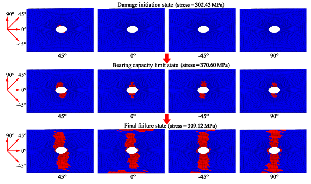
Figure 10. Illustration of delamination damage evolution at four plies of the second sub-laminate in different loading states.

As shown in Figure 10, delamination damage began at the notch edge of the 45° ply at a tensile stress of 302.43 MPa. The damage then quickly extended to the notch edges of the other three plies and spread along the Y-axis from the circular notch to the ply sides. In the final failure state, the delamination became distributed around the notch and almost penetrated the entire laminate cross-section.

From the illustrations of the three types of damage evolutions above, one can see that the FRP laminate could still bear the increasing load after damage initiation, even in the fibre damage mode case. In the final failure state, the three types of damages were fully extended at the cross-sections near the notch. In general, the damage evolutions of the laminate obtained by numerical modelling coincided well with the observation results of the verification experiment.

4. Case Study 2: Bolted FRP Laminate under Unidirectional Tension

4.1. Geometry and Material Properties

The specimen studied in this case was the carbon fibre-reinforced polymer (CFRP) laminate with a single bolted joint. Its diagrammatic sketch and geometry information are shown in Figure 11.

Figure 11. Diagrammatic sketch and geometry of the CFRP laminate specimen.

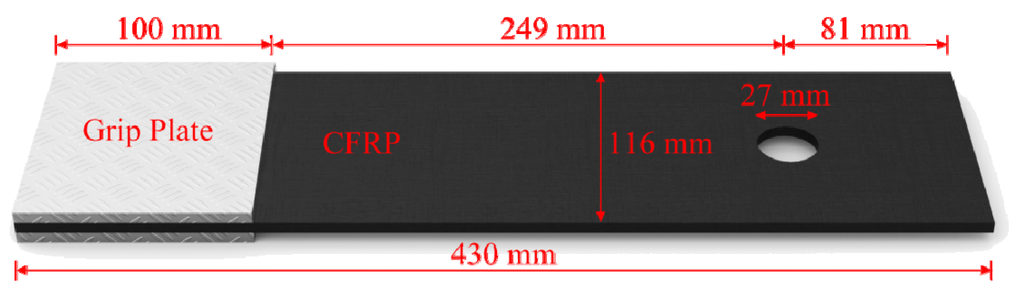
Figure 11. Diagrammatic sketch and geometry of the CFRP laminate specimen.

The laminate was made of CFRP prepregs from the SGL Group in an autoclave process. The fibre used was the SGL C30 carbon fibre, and the polymer was the epoxy-based resin. The specimen had a fibre content of 52% and a stacking sequence of . The thickness of each ply was 0.25 mm, and the total thickness of the laminate was 5.25 mm. The material properties of a single ply are listed in Table 5.

Table 5. Material properties of the specimen (each ply).

Elastic property	Value	Strength property *	Value
E1	116,000 MPa		2,160 MPa
E2 = E3	7,500 MPa		1,900 MPa
G12= G13	3,000 MPa		80 MPa
G23	2,800 MPa		210 MPa
v12 = v13	0.3	S12= S13	110 MPa
v23	0.33	S23	90 MPa

Note: * the strain limits ε_ij are equal to s_ij / c_ij (i = 1,2,3).

Table 5. Material properties of the specimen (each ply).

Elastic property	Value	Strength property *	Value
E1	116,000 MPa		2,160 MPa
E2 = E3	7,500 MPa		1,900 MPa
G12= G13	3,000 MPa		80 MPa
G23	2,800 MPa		210 MPa
v12 = v13	0.3	S12= S13	110 MPa
v23	0.33	S23	90 MPa

Note: * the strain limits ε_ij are equal to s_ij / c_ij (i = 1,2,3).

4.2. Experimental Set-Up

The corresponding experiment was conducted in a laboratory at the Technical University of Berlin. Two CFRP laminate specimens were tested. They were clamped at one end and a single bolt joint was positioned at the other end. The details of the specimens and the experimental set-up are shown in Figure 12.

As shown in Figure 12, besides the finger-tight steel bolt and nut, steel washers and spacers were also used to adjust the spacing and to maintain the correct tensile direction. Specifically, in accordance with the Eurocode (DIN EN 14399), the ratio between the diameters of washer and bolt was D_w/D = 1.85 [43]. A universal testing machine (Instron 8502) was used to pull the specimens. The loading velocity was set to 1 mm/s. Load cells and displacement sensors recorded the tension force and deformation.

Figure 12. Part section view of the specimen and the experimental set-up.

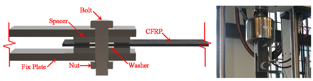
Figure 12. Part section view of the specimen and the experimental set-up.

4.3. Finite Element Model

The experimental model was simplified for the finite element calculations. The simplified calculation model that includes fibre orientation coordinates and load and boundary conditions is shown in Figure 13.

Figure 13. Schematic of the simplified calculation model with fibre orientation coordinates, load conditions and boundary conditions.

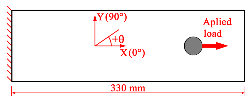
Figure 13. Schematic of the simplified calculation model with fibre orientation coordinates, load conditions and boundary conditions.

Based on the above simplified calculation model, the FE model was created in the general FEM software ABAQUS. Considering both the calculation accuracy and the speed, the steel part of the single bolt joint was simplified to a model including only the bolt and the washer. For both CFRP and steel, a three-dimensional solid 8-node linear element C3D8 was adopted. Surface-to-surface contact technology with a friction coefficient of 0.1 was adopted to simulate the interaction between the CFRP part and the steel part. To conduct the progressive damage analysis, the same degradation method with the CDM-based exponential damage factors using the damage index as the key independent variable introduced in Section 3.3.2 was applied. Because stress concentrations were expected near the notch, the mesh in this zone was refined. Furthermore, because of the symmetrical stacking, only half of the specimen was modelled. The FE model is shown in Figure 14.

Additionally, another similar FE model was established to investigate the influence of cohesive layers. In this model, delamination was considered and controlled by the cohesive layers, which were composed of cohesive elements. The geometrical thickness of these layers was set to 1% of that for the single ply: 0.0025 mm. Therefore, the thickness of CFRP plies was slightly reduced. Specifically, the outer ply and the inner plies were set to 99.5% and 99% of their original thicknesses, respectively.

Figure 14. FE model of the bolted CFRP laminate specimen with the global coordinate system.

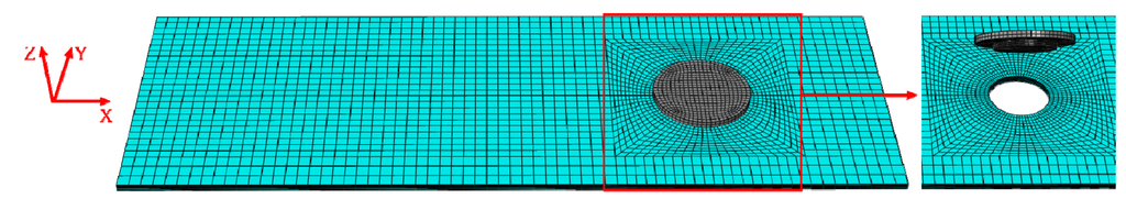
Figure 14. FE model of the bolted CFRP laminate specimen with the global coordinate system.

The ABAQUS built-in cohesive element was adopted in this paper, which complied with the traction-separation law. This traction-separation law before damage initiation can be written as [28]:

(30)

In the above equation, t_i (i = n,s,t) represent three nominal tractions in the normal direction and two shear directions, respectively. ε_i (i = n,s,t) represent the corresponding three nominal strains. K_ij (i = n,s,t) are the interface stiffness values in the interface stiffness matrix [28].

The above-mentioned traction-separation law can be uncoupled or coupled. When uncoupled, only K_nn, K_ss and K_tt must be defined, and the off-diagonal terms of the matrix are zero. When coupled, all components in the interface stiffness matrix must be defined.

Some studies have demonstrated that coupling is important in this traction-separation model [29,30]. However, other studies have shown that the uncoupled model achieved sufficient calculation accuracy and it is difficult to determine the values of the off-diagonal terms in the matrix, namely, K_ns, K_nt and K_st [44,45,46]. In general, the coupled model is used in research focusing on the cohesive zone. The uncoupled model is widely used in other cases, such as investigating the mechanical behaviour of an entire laminate specimen.

In this paper, the research focus was on the composite laminate instead of on the cohesive zone. Therefore, cohesive elements with uncoupled traction-separation law were adopted. Based on (30), the constitutive behaviour of the cohesive elements used can be written as:

(31)

The real thicknesses of the cohesive layers T_g can be used to determine the interface stiffness values, as proposed by Daudeville [47]:

(32)

(33)

E and G, which are the matrix material properties, were set to 2400 and 1000 MPa. T_g was 0.0025 mm.

The failure stresses of the cohesive material were also derived from the matrix property, and . The cohesive element damage initiation was controlled by the ABAQUS built-in quadratic nominal strain criterion:

(34)

where , and .

After damage initiation was reached, the material properties of the cohesive elements would also be exponentially degraded by the ABAQUS built-in exponential damage factors. Mixed-mode behaviour was also accounted for during damage evolution. A complete description of the cohesive element used in this paper is given in [28].

The FE model with cohesive layers is shown in Figure 15:

Figure 15. FE model of the bolted CFRP laminate specimen containing cohesive layers with the global coordinate system.

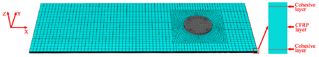
Figure 15. FE model of the bolted CFRP laminate specimen containing cohesive layers with the global coordinate system.

4.4. Comparison of Numerical and Experimental Results

The numerical and experimental bearing stress–bearing strain results are shown in Figure 16. The bearing stress is defined as , where P is the applied load, d is the hole diameter and h is the specimen thickness. The bearing strain is defined as ε_Br = δ / d, where δ is the bolt displacement. The bearing strength is defined as , where P_ultimate is the ultimate load [22].

Figure 16. Experimental versus numerical bearing stress-bearing strain responses.

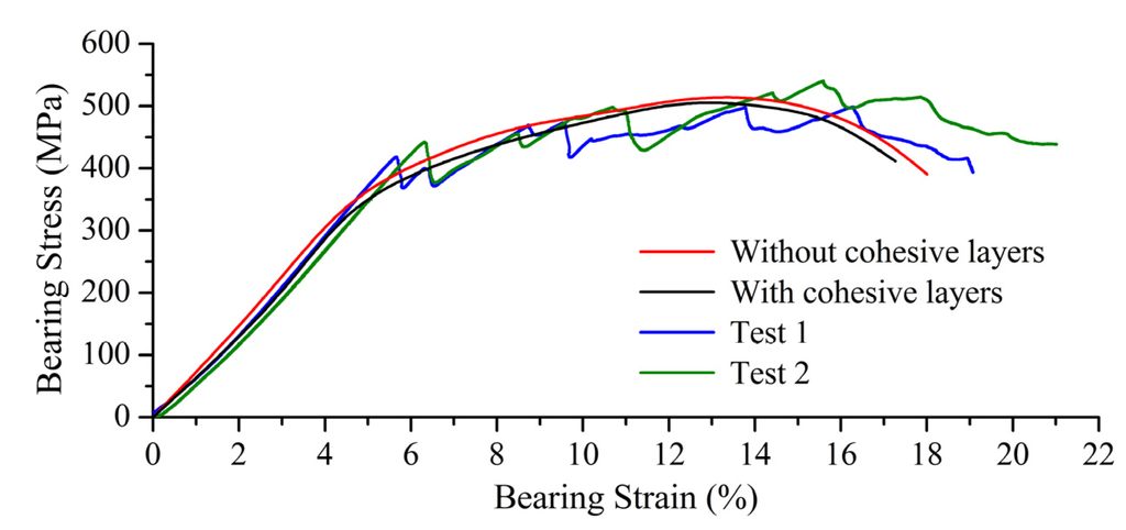
Figure 16. Experimental versus numerical bearing stress-bearing strain responses.

Figure 16 shows that numerical results with and without cohesive layers generally coincide with the experimental results. The ultimate strength obtained from the FE model without cohesive layers was almost identical to that from the model with cohesive layers (Table 6). This shows that the three-dimensional strain strength criterion proposed in this paper is accurate enough to predict the damage initiations of fibre, matrix and delamination in the case of in-plane loading of FRP laminates.

Table 6. Comparison of bearing strengths obtained by tests and numerical calculations.

FE model	Numerical result	Test 1 result	Error 1	Test 2 result	Error 2
Without cohesive layers	509.42 MPa	498.98 MPa	2.09%	540.32 MPa	−5.72%
With cohesive layers	502.22 MPa		0.65%		−7.05%

Table 6. Comparison of bearing strengths obtained by tests and numerical calculations.

FE model	Numerical result	Test 1 result	Error 1	Test 2 result	Error 2
Without cohesive layers	509.42 MPa	498.98 MPa	2.09%	540.32 MPa	−5.72%
With cohesive layers	502.22 MPa		0.65%		−7.05%

Because the numerical results from these two FE models were similar, and because omitting the cohesive layers would considerably simplify the pre-processing and the post-processing in the finite element analysis, the following numerical results are based on the FE model without cohesive layers.

The deformation and damage distribution from the numerical calculation in the final failure state are compared with the test results in Figure 17, wherein the red zones indicate the damaged zones and the blue zones indicate no damage.

Figure 17. Deformation and damage distribution at the specimen in the final failure state with the fibre orientation coordinate.

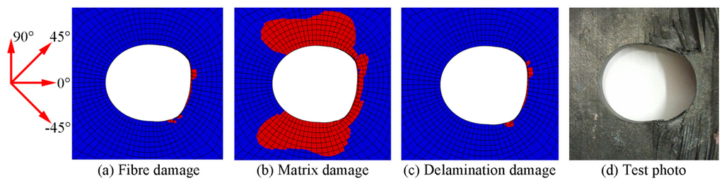
Figure 17. Deformation and damage distribution at the specimen in the final failure state with the fibre orientation coordinate.

As shown in Figure 17, the fibre, matrix and delamination damage existed at or near the circular notch. In the final failure state, a large area of fibre failure occurred at the compression side of the notch. This directly caused the final destruction of the bolted CFRP laminate. The resulting failure was a typical bearing failure. This was verified by the experiment.

The fibre, matrix and delamination damage evolutions of the laminate are shown in Figure 18, Figure 19 and Figure 20, respectively. Because the damage evolutions at two of the [−45 / 0 / 45 / 90] sub-laminates were similar, only the damage diagrams for the one closer to the middle plane, the sub-laminates [45 / 90] and the middle 0° ply are listed according to the stacking sequence in the following figures. Each of the figures displays the damage evolution at different sub-laminate plies in three loading states: the damage initiation state, the bearing capacity limit state and final failure state. Their definitions have been described in Section 3.4.

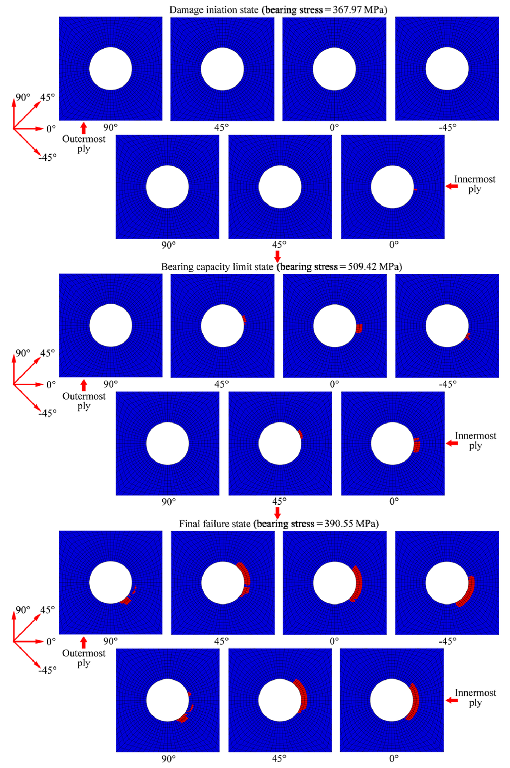
Figure 18. Illustration of fibre damage evolution at seven plies (sub-laminate [−45 / 0 / 45 / 90], [45 / 90] and middle 0° ply) in different loading states.

Figure 18. Illustration of fibre damage evolution at seven plies (sub-laminate [−45 / 0 / 45 / 90], [45 / 90] and middle 0° ply) in different loading states.

Figure 19. Illustration of matrix damage evolution at seven plies (sub-laminate [−45 / 0 / 45 / 90], [45 / 90] and middle 0° ply) in different loading states.

Figure 19. Illustration of matrix damage evolution at seven plies (sub-laminate [−45 / 0 / 45 / 90], [45 / 90] and middle 0° ply) in different loading states.

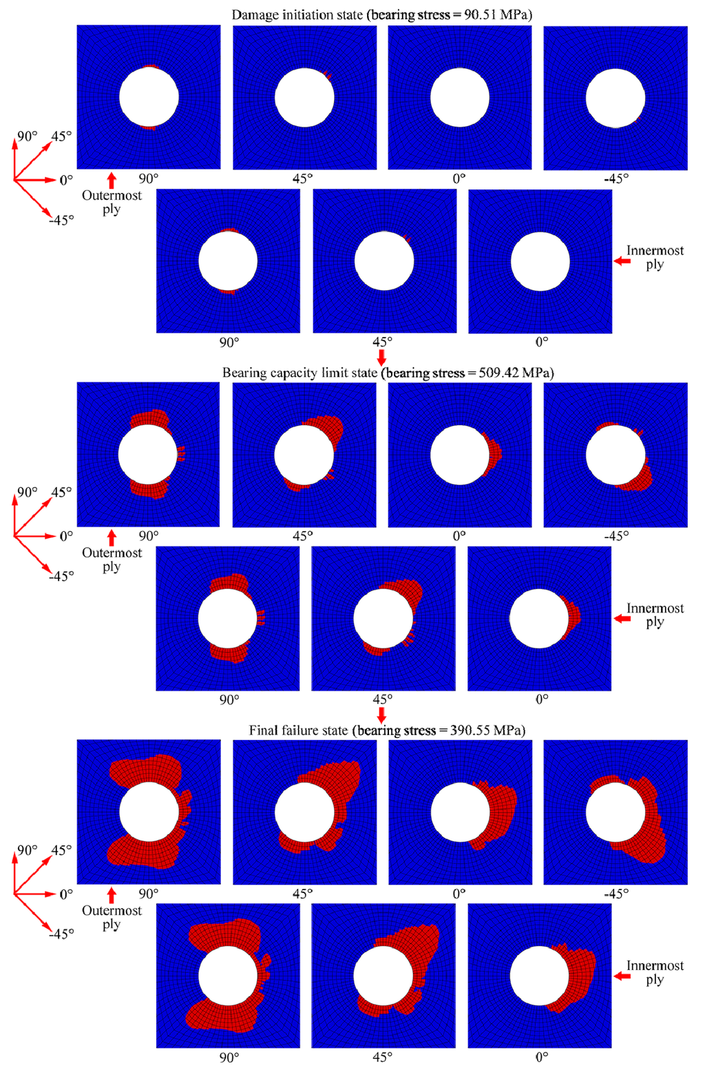
Figure 20. Illustration of delamination damage evolution at seven plies (sub-laminate [−45 / 0 / 45 / 90], [45 / 90] and middle 0° ply) in different loading states.

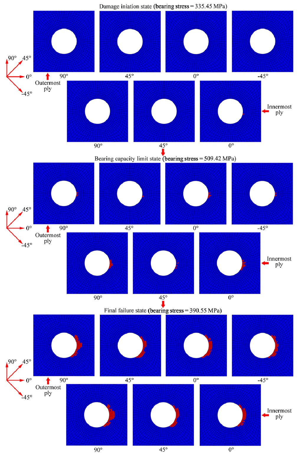
Figure 20. Illustration of delamination damage evolution at seven plies (sub-laminate [−45 / 0 / 45 / 90], [45 / 90] and middle 0° ply) in different loading states.

Figure 18 shows that the fibre damage first occurred at the compression side of the notch at the innermost 0° ply at a bearing stress of 367.97 MPa. The outer 0° ply was damaged at the same location soon after. The fibre damage then spread to the 45° and −45° plies. When the bolt joint bearing capacity (bearing stress = 509.42 MPa) had been reached, fibre damage appeared in all plies except in the two 90° plies. As the load continued to increase, the damage also spread to the 90° plies and to the compression sides of the notches in each ply. Finally, a large area of fibre damage occurred in this region, which caused the final destruction of the laminate. In the failure process, the damage areas in the 0° plies were always the largest, whereas those in the 90° plies were always the smallest under identical tensile loads.

Figure 19 shows that the matrix damage initiated at the notches of the 90° plies at a bearing stress of 90.51 MPa. The damage then quickly spread to the 45° and −45° plies. The damage then extended symmetrically in a butterfly-like shape in the 90° plies along the Y-axis. In the 45° and −45° plies, the damage mainly spread along a 45° and −45° angle from the X-axis, respectively. In the 0° plies, the matrix damage first occurred at the compression side of the notch and then extended along the X-axis as the load increased. In the failure process of the laminate, the damage areas in the two 90° plies were always larger than those in the 45°, 0° and −45° plies under identical applied loads.

Figure 20 shows the delamination damage evolution in the laminate. The delamination damage first occurred at the compression side of the notch in the innermost 0° ply at a bearing stress of 335.45 MPa. The damage then quickly spread to the same location in other plies. The delamination extended relatively slowly in the laminate until the bearing capacity of the bolt joint was reached, mainly because of the effect of the washer. After that, it extended quickly in each ply until the laminate was destroyed. In the final failure state, the delamination areas in the 90° plies were larger than those in other plies and had reached the edge of the washer.

The above progressive damage analysis has demonstrated that the single bolted CFRP laminate has good ductility. The deformation of the laminate from the initial damage, even in the fibre damage mode, to the final failure was longer than its elastic deformation. The washer played a considerable role in controlling the delamination damage by preventing the delamination from fully extending in an early stage. The ultimate strength and the failure process of the bolted laminate were in good agreement with the results of the verification experiment.

4. Conclusions

Based on the damage mechanics, a three-dimensional FE model was created in the general FEM software ABAQUS to perform the nonlinear progressive damage analyses of notched or bolted FRP laminates. A three-dimensional strain strength criterion was proposed and adopted in this model to predict damage initiation in the laminates. A damage tensor constituted by damage factors was applied to degrade material properties after damage had occurred. The results from using various damage factors were compared for accuracy and convergence. These factors included constant damage factors, CDM-based exponential damage factors that used the damage index as the key independent variable and CDM-based exponential damage factors that used the square index. The influence caused by the absence or presence of cohesive layers in the model was also explored. Throughout this paper, the progressive damage analysis of composite materials is presented and the selection of some key parameters in the analysis is discussed. Key conclusions drawn from this work are:

• The numerical results based on the three-dimensional strain strength criterion proposed in this paper are in good agreement with the experimental results. This shows that this succinct strain strength criterion is suitable for using in industry and research to predict the ultimate strengths of notched or bolted FRP laminates.
• The damage tensor used in this paper, which is strictly derived from the basic theory of damage mechanics, consists of damage factors. It is suitable for degrading the FRP material properties according to different damage modes. It was also found that the CDM-based exponential damage factors using the damage index as the independent variable are preferable to the similar CDM-based exponential damage factors using the square index as the independent variable and the conventional constant damage factors. This preferred type of exponential damage factors was controlled by the damage index k as well as the fracture energy. These factors gave the best accuracy and convergence in the numerical model compared to the results gained by the exponential damage factors using the square index f, which has no clear physical concept, and the constant damage factors, which are set empirically.
• Many existing studies demonstrate that the calculation model for composite materials with cohesive layers probably performs better than the model without cohesive layers, particularly in some complex cases. However, in the case of in-plane FRP laminate loading, such as notched or bolted FRP laminates under unidirectional tension, the three-dimensional strain strength criterion proposed in this paper shows sufficient accuracy. Adding cohesive layers to the model to simulate the delamination damage will considerably increase the amount of work necessary for pre-processing and post-processing, with limited increase in calculation accuracy.

References

- Mallick, P. Fiber-Reinforced Composites: Materials, Manufacturing, and Design, 2nd ed.; CRC Press: New York, NY, USA, 1993; pp. 6–7. [Google Scholar]
- Schlaich, M.; Zwingmann, B.; Liu, Y.; Goller, R. CFRP tension elements and their anchorages. Bautechnik 2012, 89, 841–849. [Google Scholar] [CrossRef]
- Hinton, M.J.; Soden, P.D. Predicting failure in composite laminates: The background to the exercise. Composit. Sci. Technol. 1998, 58, 1001–1010. [Google Scholar] [CrossRef]
- Hinton, M.J.; Kaddour, A.S. The background to part b of the second world-wide failure exercise: Evaluation of theories for predicting failure in polymer composite laminates under three-dimensional states of stress. J. Composit. Mater. 2013, 47, 643–652. [Google Scholar] [CrossRef]
- Whitney, J.M.; Nuismer, R.J. Stress fracture criteria for laminated composites containing stress-concentrations. J. Composit. Mater. 1974, 8, 253–265. [Google Scholar] [CrossRef]
- Karlak, R.F. Hole effects in a related series of symmetrical laminates. In Proceedings of the Conference on Failure Modes in Composite (IV), Chicago, IL, USA, 1–3 January 1977.
- Pipes, R.B.; Wetherhold, R.C.; Gillespie, J.W. Notched strength of composite-materials. J. Composit. Mater. 1979, 13, 148–160. [Google Scholar] [CrossRef]
- Echaabi, J.; Trochu, F.; Gauvin, R. Review of failure criteria of fibrous composite materials. Polym. Composit. 1996, 17, 786–798. [Google Scholar] [CrossRef]
- Chamis, C.C. Polymer composite mechanics review—1965 to 2006. J. Reinf. Plast. Composit. 2007, 26, 987–1019. [Google Scholar] [CrossRef]
- Hashin, Z. Failure criteria for unidirectional fiber composites. J. Appl. Mech. Trans. Asme 1980, 47, 329–334. [Google Scholar] [CrossRef]
- Puck, A. A failure criterion shows the direction. Kunststoffe-German Plast. 1992, 82, 607–610. [Google Scholar]
- Chang, F.K.; Chang, K.Y. A progressive damage model for laminated composites containing stress-concentrations. J. Composit. Mater. 1987, 21, 834–855. [Google Scholar] [CrossRef]
- Chang, F.K.; Lessard, L.B. Damage tolerance of laminated composites containing an open hole and subjected to compressive loadings: 1. Analysis. J. Composit. Mater. 1991, 25, 2–43. [Google Scholar]
- Tan, S.C. A progressive failure model for composite laminates containing openings. J. Composit. Mater. 1991, 25, 556–577. [Google Scholar]
- Tan, S.C.; Perez, J. Progressive failure of laminated composites with a hole under compressive loading. J. Reinf. Plast. Composit. 1993, 12, 1043–1057. [Google Scholar] [CrossRef]
- Camanho, P.P.; Matthews, F.L. A progressive damage model for mechanically fastened joints in composite laminates. J. Composit. Mater. 1999, 33, 2248–2280. [Google Scholar] [CrossRef]
- Shokrieh, M.M.; Lessard, L.B. Progressive fatigue damage modeling of composite materials, part i: Modeling. J. Composit. Mater. 2000, 34, 1056–1080. [Google Scholar]
- Shokrieh, M.M.; Lessard, L.B. Progressive fatigue damage modeling of composite materials, part ii: Material characterization and model verification. J. Composit. Mater. 2000, 34, 1081–1116. [Google Scholar]
- Tserpes, K.I.; Labeas, G.; Papanikos, P.; Kermanidis, T. Strength prediction of bolted joints in graphite/epoxy composite laminates. Composit. B Eng. 2002, 33, 521–529. [Google Scholar] [CrossRef]
- Lapczyk, I.; Hurtado, J.A. Progressive damage modeling in fiber-reinforced materials. Composit. A Appl. Sci. Manuf. 2007, 38, 2333–2341. [Google Scholar] [CrossRef]
- Linde, P.; de Boer, H. Modelling of inter-rivet buckling of hybrid composites. Composit. Struct. 2006, 73, 221–228. [Google Scholar] [CrossRef]
- Frizzell, R.M.; McCarthy, C.T.; McCarthy, M.A. Simulating damage and delamination in fibre metal laminate joints using a three-dimensional damage model with cohesive elements and damage regularisation. Composit. Sci. Technol. 2011, 71, 1225–1235. [Google Scholar] [CrossRef]
- Dugdale, D.S. Yielding of steel sheets containing slits. J. Mech. Phys. Solids 1960, 8, 100–104. [Google Scholar] [CrossRef]
- Barenblatt, G.I. The mathematical theory of equilibrium cracks in brittle fracture. Adv. Appl. Mech. 1962, 7, 55–129. [Google Scholar] [CrossRef]
- Needleman, A. A continuum model for void nucleation by inclusion debonding. J. Appl. Mech. Trans. Asme 1987, 54, 525–531. [Google Scholar] [CrossRef]
- Needleman, A. An analysis of tensile decohesion along an interface. J. Mech. Phys. Solids 1990, 38, 289–324. [Google Scholar] [CrossRef]
- Camanho, P.P.; Davila, C.G.; de Moura, M.F. Numerical simulation of mixed-mode progressive delamination in composite materials. J. Composit. Mater. 2003, 37, 1415–1438. [Google Scholar] [CrossRef]
- Systèmes, D. ABAQUS 6.10: Analysis User’s Manual; Dassault Systèmes Simulia Corp: Providence, RI, USA, 2010. [Google Scholar]
- Goutianos, S.; Sørensen, B.F. Path dependence of truss-like mixed mode cohesive laws. Eng. Fract. Mech. 2012, 91, 117–132. [Google Scholar] [CrossRef]
- McGarry, J.P.; Ó Máirtín, É.; Parry, G.; Beltz, G.E. Potential-based and non-potential-based cohesive zone formulations under mixed-mode separation and over-closure. Part I: Theoretical analysis. J. Mech. Phys. Solids 2014, 63, 336–362. [Google Scholar] [CrossRef]
- Máirtín, ÉÓ; Parry, G.; Beltz, G.E.; McGarry, J.P. Potential-based and non-potential-based cohesive zone formulations under mixed-mode separation and over-closure—part ii: Finite element applications. J. Mech. Phys. Solids 2014, 63, 363–385. [Google Scholar] [CrossRef]
- Perugini, P.; Riccio, A.; Scaramuzzino, F. Three-dimensional progressive damage analysis of composite joints. In Proceedings of the 8th International Conference on Civil and Structural Engineering Computing, Vienna, Austria, 19–21 September 2001.
- Tserpes, K.; Papanikos, P.; Kermanidis, T. A three-dimensional progressive damage model for bolted joints in composite laminates subjected to tensile loading. Fatigue Fract. Eng. Mater. Struct. 2001, 24, 663–675. [Google Scholar] [CrossRef]
- Tsai, S.W. Theory of Composites Design; Think Composites: Dayton, OH, USA, 1992. [Google Scholar]
- Krajcinovic, D. Damage Mechanics; Elsevier: Waltham, MA, USA, 1996; Volume 41. [Google Scholar]
- Ladevèze, P.; Simmonds, J.G. Nonlinear Computational Structural Mechanics: New Approaches and Non-incremental Methods of Calculation; Springer: Berlin, Germany, 1999; pp. 11–12. [Google Scholar]
- Liu, P.F.; Zheng, J.Y. Recent developments on damage modeling and finite element analysis for composite laminates: A review. Mater. Des. 2010, 31, 3825–3834. [Google Scholar] [CrossRef]
- Burr, A.; Hild, F.; Leckie, F.A. Micromechanics and continuum damage mechanics. Arch. Appl. Mech. 1995, 65, 437–456. [Google Scholar]
- Zienkiewicz, O.C.; Taylor, R.L. The Finite Element Method: Solid Mechanics, 6rd ed.; Butterworth-heinemann: Oxford, UK, 2000; Volume 2, pp. 4–37. [Google Scholar]
- O’Higgins, R.M.; McCarthy, M.A.; McCarthy, C.T. Comparison of open hole tension characteristics of high strength glass and carbon fibre-reinforced composite materials. Composit. Sci. Technol. 2008, 68, 2770–2778. [Google Scholar] [CrossRef]
- Wang, Y.; Tong, M.; Zhu, S. Three-dimensional nonlinear progressive damage analysis on composite laminates based on continuum damage mechanics. J. Nanjing Univ. Aeronaut. Astronaut. 2009, 6, 709–714. [Google Scholar]
- ASTM Standard D5766/D5766M-02. Standard test method for open hole tensile strength of polymer matrix composite laminates. In Annual Book of ASTM Standards; ASTM International: West Conshohocken, PA, USA, 2002; Volume: 15.03.
- Deutsches Institut für Normung. DIN EN 14399: High-Strength Structural Bolting Assemblies for Preloading; Beuth: Berlin, Germany, 2005. [Google Scholar]
- Jin, Z.-H.; Sun, C. Cohesive zone modeling of interface fracture in elastic bi-materials. Eng. Fract. Mech. 2005, 72, 1805–1817. [Google Scholar] [CrossRef]
- Park, K.; Paulino, G.H. Computational implementation of the ppr potential-based cohesive model in abaqus: Educational perspective. Eng. Fract. Mech. 2012, 93, 239–262. [Google Scholar] [CrossRef]
- Alves, J.L.; Roehl, D. A new cohesive zone model for shell. In Proceedings of the 12th Pan-American Congress of Applied Mechanics, Port of Spain, Trinidad, 2–6 January 2012.
- Daudeville, L.; Allix, O.; Ladeveze, P. Delamination analysis by damage mechanics—Some applications. Compos. Eng. 1995, 5, 17–24. [Google Scholar] [CrossRef]
© 2014 by the authors; licensee MDPI, Basel, Switzerland. This article is an open access article distributed under the terms and conditions of the Creative Commons Attribution license (http://creativecommons.org/licenses/by/3.0/).