Historical Perspective of Advances in the Science and Technology of Polymer Blends

Abstract

This paper will review the important developments in the field of polymer blends. The subject of polymer blends has been one of the most prolific areas in polymer science and technology in the past five decades judging from publications and patents on the subject. Although a continuing important subject, the peak intensity occurred in the 1970s and 1980s. The author has been active in this area for five decades and this paper is a recollection of some of the important milestones/breakthroughs in the field. The discussion will cover the development of the theory relevant to polymer blends, experimental methods, approaches to achieve compatibility in immiscible/incompatible blends, the nature of phase separation and commercial activity.

1. Introduction

The area of polymer blends has been a major topic of polymer research and development for almost five decades. Although noted to be of interest much earlier, the academic and industrial effort in polymer blends exponentially increased starting in the late 1960s. Although various reasons were responsible for this increased interest, one significant factor was the emergence of a major engineering polymer blend based on polystyrene (specifically impact polystyrene) and poly(2,6-dimethyl-1,4-phenylene oxide) (PPO). The miscibility of this blend allowed for useful properties over the composition range. This discovery at General Electric [1] resulted in the commercial introduction of a myriad of blends under the tradename Noryl^®. While the industrial impact is obvious, the academic interest was significant. Miscibility in polymer blends was considered a much unexpected behavior up to that point in time. The observation of miscibility for polystyrene and PPO (where no obvious strong interaction exists) led to numerous academic studies directed towards understanding polymer miscibility. Another reason for the surge in polymer blend activity was the recognition that polymeric blends (alloys) could have an analogous importance that had been demonstrated for metal alloys. The in-situ-polymerization of styrene in the presence of rubber to produce impact polystyrene and also styrene/acrylonitrile polymerization with rubber to yield poly(acrylonitrile butadiene styrene) (ABS) had become major polymeric products. This process (developed in the 1950s) gave much better properties than simple mixtures of polystyrene or styrene/acrylonitrile copolymers with rubber [2]. By the 1960s, it was also recognized that mixtures of different rubbers gave improved tire properties over any specific unblended rubber composition. One of the earliest commercial examples (early 1940s) of miscible polymer blends involved the mixture of poly(vinyl chloride) (PVC) and butadiene-acrylonitrile rubber yielding a permanently plasticized PVC [3,4].

This paper will discuss the significant historical advances in the science and technology of polymer blends with emphasis on the developments occurring in the 1970s and 1980s when the peak activity in both academic and industrial research occurred. Although a significant amount of research activity in that time period involved understanding the nature of miscibility in polymer blends, significant advances were also accomplished in developing the technology for polymer blend compatibilization of immiscible and incompatible components. The theoretical framework for polymer blend thermodynamics will be reviewed and the important advances in the experimental methods for assessing the thermodynamic interactions (e.g., heat of mixing).

2. Theory: Review of Historical Developments

2.1. Flory-Huggins Equation

The basic thermodynamic relationship governing mixtures established by Gibbs [5] is:

ΔG_m = ΔH_m − TΔS_m

(1)

where ΔG_m = the free energy of mixing, ΔH_m = the enthalpy of mixing and ΔS_m = the entropy of mixing with T being the temperature. For mixing (miscibility) to occur, ΔG_m < 0. This is a necessary criterion, but is not sufficient as the equation below must also be met:

(2)

The basic theory for assessing the miscibility of polymer blends was developed by Flory [6,7] and Huggins [8,9] and is thus referred to as the Flory-Huggins theory. The equation resulting from their analysis is termed the Flory-Huggins Equation as noted:

(3)

where V = total volume, V_i = molecular volume of component i, φ_i = volume fraction of component i, k = Boltzman’s constant, χ₁₂ = Flory-Huggins interaction parameter and υ_r = interacting segment volume (such as a repeat unit volume) and is also referred to as the reference volume. This equation was primarily employed for solvent-polymer mixtures but is applicable to higher molecular weight polymer mixtures.

The Flory-Huggins Equation was successfully applied to demonstrate the basic reason for decreased miscibility of solvent-polymer mixtures compared to solvent-solvent mixtures as the combinatorial entropy of mixing is decreased. With polymer-polymer mixtures, the combinatorial entropy of mixing approaches insignificant values in the limit of high molecular weight polymer mixtures. Thus to achieve miscibility, a negative heat of mixing must be obtained (i.e., χ₁₂ < 0).

2.2. Solubility Parameter Concept

The solubility parameter concept allows for a predictive capability of assessing the potential of miscibility of liquids. The concept traces back to Hildebrand [10] where the solubility of a material was noted to be influenced by the solvent internal pressure. This concept was further developed by Scatchard [11]. Scatchard defined the cohesive energy density as the energy of vaporization per unit volume Hildebrand and Scott [12] then defined the solubility parameter (δ_p) as the square root function of the cohesive energy density:

(4)

The basic concept involves matching the solubility parameter to achieve miscibility. For solvent-solvent mixtures, the solubility parameter difference can be rather large for miscibility to be achieved. With solvent-polymer mixtures, the solubility parameter difference is much lower to achieve miscibility but still significant. This approach works quite well for non-polar solvent mixtures with some divergence for highly polar or hydrogen bonding liquids as well as other specifically interacting molecules. With polymer-polymer mixtures, the solubility parameters need to be virtually identical to achieve miscibility in the absence of strong polar or hydrogen bonding interactions. With polymers, the energy of vaporization cannot be determined. The polymer solubility parameter is typically determined by swelling a crosslinked sample in a series of solvents and assigning the solubility parameter value where the highest swelling (best solvent) occurs. In order to address polar and hydrogen bonding polymers, three dimensional solubility parameters were proposed by Hansen [13] and has found utility for solvent-polymer mixtures but limited applicability for polymer-polymer mixtures.

An approach which has been useful for predicting the solubility parameter for polymers involves a group contribution method. The most utilized approach is by Small [14] with additional approaches noted by van Krevelan [15], Hoy [16] and Coleman [17]. While the solubility parameter approach has some qualitative utility, the inability to address specific interactions is a major limitation. The relationship of Flory-Huggins interaction parameter with the solubility parameter is:

(5)

and thus negative values (indicative of specific interactions) cannot be obtained.

2.3. Equation of State (EOS)

An equation of state (EOS) is typically a mathematical relationship between several variables most commonly employed with pressure, volume and temperatures of gases. The equation of state approach can also be applied to liquid and polymer systems. Prigogine developed an equation of state for liquid mixtures [18]. Flory developed an equation of state for solvent-polymer mixtures following the formalism developed by Prigogine but accounting for chain segments to accommodate polymers [19,20,21]. These approaches employ reduced pressure, reduced volume, reduced temperature and a partition function to describe the system. The Flory equation of state approach allows for compressibility effects whereas the Flory-Huggins lattice model (Equation 3) is an incompressible model. This difference can lead to conditions that allow the equation of state approach to predict lower critical solution temperature (LCST) behavior. The lattice model can only predict this if the Flory-Huggins interaction parameter is temperature dependant.

McMaster [22] applied the Flory EOS approach to polymer-polymer mixtures and investigated the effect of key variables on the predicted phase behavior. It was found that LCST behavior was predicted for polymer-polymer blends and probably the expected case. The temperature dependence of the thermal expansion coefficient, the thermal pressure coefficient and the interaction coefficient (related to the Flory-Huggins interaction parameter) showed the effect of these variables on the temperature-composition phase diagrams. The prediction that LCST behavior would be prevalent for polymer blends was unexpected at that point as the conventional wisdom was that increasing temperature would increase miscibility. Experimental data on polymer blends exhibiting LCST behavior was virtually non-existent except for an observation by Shaw [23]. Further studies after this publication confirmed that LCST behavior was prevalent for polymer blends.

Other equation of state approaches applied to polymer blends include the Sanchez-Lacombe lattice fluid theory [24,25], the Simha-Somcynsky hole theory [26], the Jain-Simha cell-hole theory [27,28], the modified cell model Dee and Walsh [29,30] and the Patterson equation of state [31]. An approach termed an oriented quasichemical approximation was proposed to better predict the phase behavior of specific interacting blends where non-random orientation is expected [32].

The EOS approaches offered significant advances in describing the variables and qualitative nature of phase behavior of polymer blends. The complexity of the approach and significant data required for specific systems however has not allowed this approach to be widely employed for predicting miscibility and phase behavior.

2.4. Mean Field Approach

An approach for predicting miscibility for homopolymer-copolymer and copolymer-copolymer blends offering significant promise was developed independently in 1973–1974 by three different research groups [33,34,35]. This approach termed the mean field binary model noted that specific segmental interactions between the monomer units of the blend were important.

In the case of a copolymer comprised of monomers where the homopolymers were highly immiscible, a case of intramolecular repulsion would result. An example involves the styrene-acrylonitrile copolymer where the homopolymers (polystyrene and polyacrylonitrile) are highly immiscible. In blends with a homopolymer (like poly(methyl methacrylate)) where the methyl methacrylate monomer unit has more favorable interactions with styrene and acrylonitrile, a window of miscibility can result. The basic equation is:

(6)

for a copolymer comprised of b and c repeat units blended with a homopolymer with repeat unit a. B_ab, B_ac and B_bc are the binary interaction density values for the specific repeat unit pairs. and are the volume fractions of b and c repeat units in the copolymer with . If B_bc is much larger than B_ab and B_ac, compositions will exist where miscibility is observed. This window of miscibility will exist if the expression below is satisfied:

(7)

As will be discussed later, B_ij values can be determined from low molecular weight analog heat of mixing data. A similar analysis can be done for copolymer-copolymer blends. This approach has shown that miscibility can be obtained in blends where no apparent specific interactions occur between the repeat unit pairs. This approach has been very successful in predicting miscibility from experimentally determined B_ij values. A myriad of miscible polymer blends based on this approach have been documented in the literature from various research groups. The University of Texas (Paul and Barlow) has provided many of these examples.

2.5. Hydrogen Bonding Fundamentals

Hydrogen bonding is an important specific interaction often noted in miscible polymer blends. Polymer blends comprised of one polymer with proton acceptor groups and another polymer with proton donor groups can have a much greater tendency to be miscible. Coleman et al. [17] noted the infrared spectra of strongly hydrogen bonded blends can be employed to predict the miscibility of these blends from an association model including a free energy contribution from specific interactions added to the Flory-Huggins equation. The formalism of employing infrared data for calculating the free energy contribution is detailed in their book and various publications.

3. Experimental Methods

3.1. Determination of χ₁₂, B₁₂, ΔH_m

For high molecular weight polymer blends, the combinatorial entropy of mixing is generally low to insignificant, thus miscibility is primarily centered on achieving negative values of χ₁₂, B₁₂, ΔH_m. Obtaining these values from direct heat of mixing is very difficult for very viscous polymer mixtures. One of the most successful methods for estimating these values is termed analog heat of mixing or analog calorimetry. This method uses low molecular weight liquids as an analog for high molecular weight polymers. This procedure recognizes that the heat of mixing is not inherently dependent on molecular weight. Heat of mixing of liquids is experimentally easy to determine by calorimetric methods. Analog compounds (such as ethyl benzene for polystyrene and acetonitrile for polyacrylonitrile) can be used to determine the heat of mixing. This method was initially developed at the University of Texas [36] and has since become the primary method for experimentally determining, χ₁₂ B₁₂, ΔH_m for polymer blends. It has been particularly useful for experimental data applied to the mean field approach discussed earlier.

The determination of χ₁₂ from melting point depression data of a crystalline polymer diluted with a miscible polymer was initially reported by Nishi and Wang [37]. The expression employed for crystalline polymer-solvent combinations applied to polymer blends is:

(8)

and are the equilibrium melting points of the blend and the undiluted crystalline polymer. υ₁ and υ₂ are the molar volumes of the miscible polymer diluents and the crystalline polymer respectively. is the heat of fusion of the crystalline polymer at 100% crystallinity and φ₂ is the volume fraction of the crystalline polymer. This method has shown good qualitative agreement with other methods employed to determine χ₁₂ for the same blends.

Small angle neutron scattering characterization of polymer blends was demonstrated by Kriste and coworkers in the 1970s [38]. Deuteration of one component of the blend is generally desired to provide contrast. This technique is particularly useful for polyolefin blends where other techniques are limited in the ability to describe the phase behavior and to determine miscibility. The Flory-Huggins interaction parameter χ₁₂ can be determined from these experiments. In the 1970s, a serious debate existed where molecular (segmental) mixing of compositionally different polymer chains was questioned. The use of the glass transition temperature to define miscibility was not uniformly accepted by the scientific community as it was not considered to be a true thermodynamic transition. A separate theory was proposed involving a “domain” size to explain the glass transition temperature behavior for “miscible” blends without the requirement of mixing of polymer molecules at the segmental level [39,40]. SANS experiments provided the experimental evidence to confirm that mixing was occurring at the molecular (segmental) level in many of the blends defined as miscible from glass transition results. Of course, compositionally different polymer blends will not approach the “ideal” molecular mixing exhibited by small molecules. Often the dynamic mechanical or calorimetric determined T_g’s of miscible blends are not as sharp as the unblended polymer component T_g’s indicating some level of heterogeneity at the segmental level.

The interaction parameter of a polymer blend can be determined from probe molecules (gas or solvent) by determining the interaction of the probe molecule with the unblended polymers compared to the polymer blend. Two methods have been employed using this analysis; vapor (or gas) sorption and inverse gas chromatography. For vapor (or gas) sorption, the Henry’s law constant of the vapor or gas is measured for the unblended polymers and the polymer blend, and the interaction parameter can be derived from the results. A comparison of this method with calorimetric and melting point depression data for the interaction energy density, B, showed good agreement [41].

The inverse gas chromatography method employs stationary supports coated with unblended polymer and the polymer blend. By measuring the vapor (or solvent) retention time, the interaction parameter of the blend can be determined. This method is at best qualitative and the results are dependent on the probe solvent chosen. One of the initial and comprehensive investigations employing this method was reported by Olabisi [42].

3.2. Experimental (Other)

Infrared spectroscopy gained prominence in the 1980s for studying hydrogen bonding in polymer blends. Specific groups capable of hydrogen bonding (hydroxyl, ester, acid, amide, amine) show frequency shifts in the presence of interacting groups (proton acceptor-proton donor interactions). This is observed with both miscible solvent-polymer mixtures as well as polymer-polymer mixtures. This observation demonstrated the ability of structurally different polymers to mix at the segmental level. Kwei et al. demonstrated that the frequency shift of polymer bound hexafluoroisopropanol groups was equivalent to unbound hexafluoroisopropanol when mixed with proton acceptors [43]. This observation demonstrated the equivalence of low and high molecular weight hydrogen bonding potential and the justification to employ analog low molecular weight compounds to assess hydrogen bonding potential in polymer blends. The most comprehensive work on infrared spectroscopy applied to polymer blends was reported by Coleman and coworkers and is summarized in a book on the subject [17].

Another novel method for demonstrating the mixing of different polymer structures at the segmental level is termed non-radiative energy transfer (NRET). A variation of this method is referred to as excimer fluorescence. The NRET method involves minor modification of the polymer components with chromophores capable of energy transfer with close proximity. Differences between the miscible and immiscible blend donor and acceptor chromophore energy transfer can be detected and also be utilized to study the phase separation process. This technique was initially noted by Morawetz [44,45]. Excimer fluorescence involves polymers containing groups capable of fluorescence (such as aromatic groups) mixed with non-fluorescent polymers. Phase separation favors fluorescence as miscibility allows separation and dilution of the fluorescent polymer chains (particularly at low levels in the polymer mixture). This method was demonstrated by Frank and coworkers [46,47].

Many other methods have been widely employed to study polymer blends. Transmission electron microscopy, scanning electron microscopy and atomic force microscopy are typically employed to study blend morphology. In addition to neutron scattering, light scattering and X-ray scattering have been widely utilized to study the level of homogeneity in polymer blends. Nuclear magnetic resonance, X-ray photoelectron spectroscopy and positron annihilation spectroscopy are additional methods worthy of mention. These methods along with dynamic mechanical, calorimetric and dielectric analysis are detailed in several books devoted to polymer blends [48,49].

4. Compatibilization of Immiscible and Incompatible Polymer Blends

Although there has been considerable interest in miscible polymer blends, the vast majority of commercial polymer blends involve immiscible combinations. Many of these combinations involve incompatible components offering poor mechanical properties unless compatibilization techniques are employed.

There are presently many compatibilization methods. Many of these techniques involve modification of the interface between the immiscible and incompatible components. If the interfacial energy can be reduced, the ability to transfer stress across the interface can be dramatically improved. This can involve addition of a ternary polymer to the blend offering good adhesion to both phases and the ability to concentrate at the interface. This behavior was best described by Hobbs et al. [50] where the interfacial tensions of a ternary polymer blend were analyzed to determine the morphology of the ternary blend and the potential for the ternary polymer to concentrate at the interface of the other two components. Graft and block copolymers of the binary components of the blend will be expected to also concentrate at the interface of the blend components. This situation leads to decreased particle size and often significant improvement in the mechanical properties. The in-situ polymerization of styrene monomer in the presence of rubber yielded much better properties for impact polystyrene than simple blends of polystyrene and rubber. Similar results were obtained for ABS and impact poly(methyl methacrylate) (PMMA).

Reactive compatibilization of incompatible polymers received considerable academic and industrial interest with the commercialization of super-tough nylon (Zytel ST: DuPont, Wilmington, DE, USA) [51]. This process involved the peroxide assisted maleic anhydride grafting onto ethylene-propylene-diene monomer (EPDM) rubber followed by blending with nylon 6 or nylon 66. The reaction of maleic anhydride with amine end group of nylon allowed for nylon grafted EPDM offering a compatibilizing interfacial component. This process could be conducted in a single pass extrusion operation. This concept was initially noted for compatibilization of polypropylene with nylon 6 [52]. Another early reactive compatibilization concept involved the extrusion polymerization of polysulfone-nylon 6 block copolymers [53]. In this case, the anionic polymerization of caprolactam in the presence of Cl-terminated polysulfone (as the initiator) and Na caprolactam as the catalyst yielded a block copolymer. This block copolymer could then be added to polysulfone, nylon 6 or polysulfone/nylon 6 blends to yield useful compositions.

The reactive extrusion concept has been demonstrated to compatibilize even the most incompatible of polymer combinations. Non-polar polyolefin compatibilization with highly polar poly(vinyl alcohol) comprises one of these examples [54]. In addition to super-tough nylon, a number of other commercial blends have been prepared via this method including Noryl GTX for automotive applications. In addition to maleic anhydride, oxazoline, carboxylic acid, epoxy and isocyanate functional groups can be grafted to polyolefins to provide reactive functionality for producing graft copolymers with other polymers. Several books are dedicated primarily to reactive compatibilization of polymers [55,56].

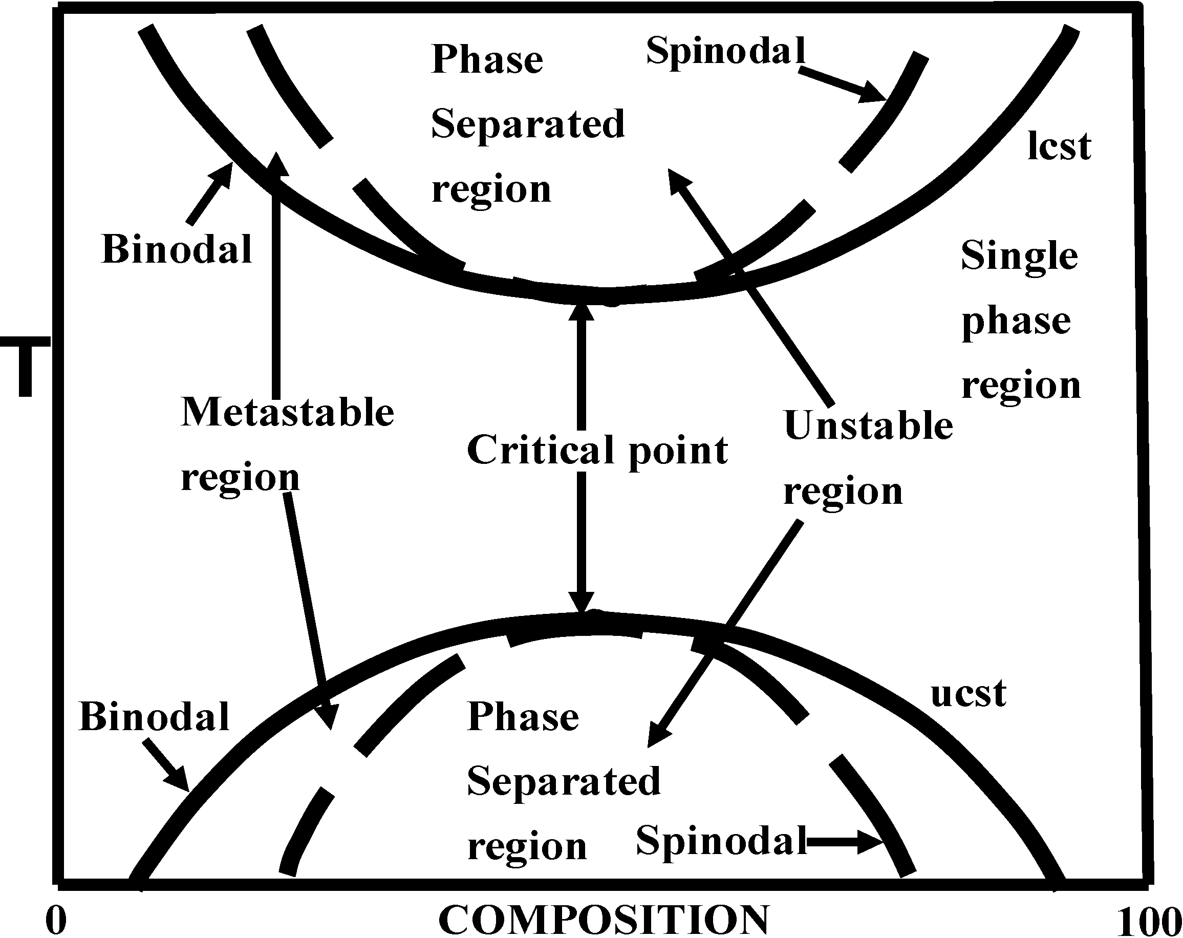
5. Phase Separation: Spinodal Decomposition versus Nucleation and Growth

Two distinctly different phase separation processes can be observed with initially miscible polymer mixtures subjected to either temperature or solvent removal (evaporation or non-solvent addition) where the phase diagram boundary is crossed. The more common process is termed nucleation and growth and the other process is called spinodal decomposition. Spinodal decomposition was observed in inorganic glasses and metal alloys prior to the initial observation with polymers by McMaster [57]. Spinodal decomposition arises from concentration fluctuations and the kinetics was initially described by Cahn and Hilliard [58,59]. Nucleation and growth is an activated process involving a location (nucleus) where phase separation occurs. The specific characteristics of the initial stages of phase separation by these processes are noted below (Table 1).

Table 1. Comparison of Phase Separation Processes.

Property	Nucleation and Growth	Spinodal Decomposition
Size of phase separated region	increases with time	size constant
Concentration of phase separated region	constant with time	increases with time
Diffusion coefficient	positive	negative
Phase structure	separated	interconnected
Activation energy	required	not required
Region of phase diagram	metastable or unstable region	only unstable region

Table 1. Comparison of Phase Separation Processes.

Property	Nucleation and Growth	Spinodal Decomposition
Size of phase separated region	increases with time	size constant
Concentration of phase separated region	constant with time	increases with time
Diffusion coefficient	positive	negative
Phase structure	separated	interconnected
Activation energy	required	not required
Region of phase diagram	metastable or unstable region	only unstable region

The relationship of these processes to the phase diagram is shown in Figure 1.

Figure 1. Phase diagram for binary polymer blend (temperature versus composition) with illustration of lower critical solution temperature (LCST) and upper critical solution temperature (UCST) behavior.

Figure 1. Phase diagram for binary polymer blend (temperature versus composition) with illustration of lower critical solution temperature (LCST) and upper critical solution temperature (UCST) behavior.

Only nucleation and growth can occur in the metastable region. Spinodal decomposition is best observed by crossing through the critical point into the unstable region without crossing the metastable region. In some cases, spinodal decomposition may result if the metastable region is rapidly crossed such that nucleation of phase separation does not occur. In addition to the observations by McMaster, another early study of spinodal decomposition was reported by Nishi et al. [60].

At the later stages of phase separation, the differences in these two processes become less obvious as phase coalescence occurs (referred to as Ostwald ripening by McMaster). Spinodal decomposition has primarily been of academic interest in polymer blends; however, the interconnected structure for solvent-polymer phase separation by non-solvent addition has had some practical interest for membrane formation processes.

6. Commercial Developments

One of the early examples of commercial polymer blends involved crosslinked phenol-formaldehyde polymers with natural rubber for phonograph records in the early 1900s [61]. One of the first commercial miscible blends was poly(vinyl chloride) with butadiene-acrylonitrile copolymers [3,4] offering permanently plasticized compositions for pit and pond liners, wire and cable insulation, gaskets and food packaging films. With the advent of synthetic rubber, elastomer blends of natural rubber and styrene-butadiene rubber were employed in the 1940s with styrene-butadiene blends with polybutadiene emerging in the 1960s for tire applications. In situ polymerication of polystyrene or styrene-acrylonitrile copolymers in the presence of rubber to yield impact polystyrene or ABS replaced simple blends of the components due to significant improvement in blend properties. An early study on the important parameters for optimizing impact polystyrene was noted by Wagner and Robeson [62]. As noted earlier, the commercialization (1967) of poly(2,6-dimethyl-1,4-phenylene oxide) (PPO) and impact polystyrene (Noryl^®: General Electric, Fairfield, CT, USA) heightened the interest in polymer blend technology. In addition to enhanced tensile strength, toughness and heat distortion temperature, the addition of PPO to impact polystyrene allowed improved flammability resistance. The addition of low cost flame retardants to the blend allowed for meeting the UL-94 V-0 rating. Underwriters Laboratories required UL-94 V-0 ratings for electrical appliances shortly after the introduction of Noryl^® opening a large market opportunity for the newly introduced blend.

ABS compositions with heat distortion temperatures >100 °C were offered in the 1960s. This was achieved by the addition of a miscible α-methyl styrene-acrylonitrile copolymer to raise the T_g of ABS. ABS/polycarbonate blends were also introduced in the 1960s by Borg-Warner under the tradename Cycoloy. This blend is phase separated but has sufficient compatibility to exhibit a property profile of commercial interest. This blend is still commercial today from other companies. Another ABS blend commercialized in the same time frame was ABS/PVC (Cycovin: Borg-Warner, Chicago, IL, USA). This compatible but phase separated blend was employed for thermoformed mass transit interiors, appliance housings and various application where ABS flame resistance was required.

The increased attention in the decade of the 1970s in polymer blend technology also saw an increase in new engineering polymer commercial blends (time frame 1970 to early 1980s). Poly(butylene terephthalate)/polycarbonate (PBT/PC) blends were introduced by General Electric under the tradename Xenoy followed by poly(ethylene terephthalate)/polycarbonate (PET/PC) blends introduced by Bayer (Macroblend). Both PBT/PC and PET/PC blends are phase separated but mechanically compatible. The phase separation allowed for retention of PBT or PET crystallinity yielding much better environmental stress rupture resistance compared to PC. Interest in polymers for automotive body panels lead to a number of engineering polymer blends. Blends were generally required as no single, unblended polymer could meet the demanding requirements. Examples of these blends included PPO/impact polystyrene/nylon 6 or 66 (Noryl GTX^®) and the PBT/PC blend (Xenoy^®). Polysulfone blends with ABS (Mindel A) and PET (Mindel B) were commercialized by Union Carbide in the late 1970s. Both blends required a minor amount of a polymeric compatibilizer to achieve the desired property profile.

Dynamically vulcanized blends of polypropylene (PP) and ethylene-propylene-diene monomer rubber (EPDM) were introduced in the 1970s (Santoprene^®: Monsanto, St. Louis, MO, USA) [63]. In this process, EPDM is the major component (by wt.) and PP/EPDM blends were extruded usually with peroxide addition to promote grafting and crosslinking of the rubber phase. As the EPDM phase is crosslinked, PP is the continuous phase. The resultant flexible product can be extruded and injection molded like a typical thermoplastic but has properties similar to a highly filled crosslinked rubber. Various versions of PP/EPDM, PP/other rubbers such as nitrile rubber, other polymers instead of PP (such as HDPE, polyamides) have been commercialized using the dynamic vulcanization concept.

An important blend combination involves polyolefin blends. Most of the information is noted either in patents or is held as trade secrets by the suppliers. Impact modification of PP by EPR or EPDM has been practiced since the 1960s. An early ternary blend involved PP (major component) with low amounts of HDPE and EPR [63]. This blend offered advantages over PP/EPR in modulus and strength without sacrificing impact strength. With the advent of linear low density polyethylene (LLDPE), initial commercial versions did not have the combination of properties to replace the conventional low density polyethylene (LDPE) for film applications. LLDPE/LDPE blends were commercially used offering a better property profile than either unblended polymer [63].

An ethylene-vinyl acetate-carbon monoxide terpolymer permanent plasticizer for PVC was introduced in the 1970s (Elvaloy: DuPont). A styrene-maleic anhydride/third monomer terpolymer miscible with styrene-acrylonitrile copolymers was commercialized in the early 1980s for ABS blends (Cadon: Monsanto) [64]. Many additional blends have been commercialized since the 1980s with examples given in [48].

7. Conclusions

The area of polymer blends has arguably been one of the most important topics in polymer science and technology in the past five decades both from an academic as well as an industrial perspective. Specific groups have had significant impact in this field. In academia, the team of Paul and Barlow at the University of Texas and Karasz and MacKnight at the University of Massachusetts deserve special recognition for their seminal work. Industrial groups at Union Carbide and General Electric are also deserving of credit along with the team of Koningsveld and Kleintjens in the Netherlands. Many other individuals and collaborative efforts have had significant impact. Many books have been published on polymer blends. In addition to those already cited, [65,66,67,68,69,70] list others covering the topics discussed above in much more detail. A book by the author of this paper [48] discusses the various subjects of this paper in detail.

References

1. Cizek, E.P. Blend of a Polyphenylene Ether and a Styrene Resin. U.S. Patent 3,383,435, 14 May 1968. [Google Scholar]
2. Henton, D.E.; Bubeck, R.A. The manufacture and physical properties of rubber-toughened styrenics. In Polymer Toughening; Arends, C.B., Ed.; Marcel Dekker: New York, NY, USA, 1996; pp. 237–291. [Google Scholar]
3. Badum, E. Ozone Resistant Cable Construction. U.S. Patent 2,297,194, 29 September 1942. [Google Scholar]
4. Henderson, D.E. Mixture of Polymerized Materials. U.S. Patent 2,330,353, 28 September 1943. [Google Scholar]
5. Gibbs, J.W. Transactions of the Connecticut Academy of Arts and Sciences; Connecticut Academy of Arts and Sciences: New Haven, CT, USA, 1873; pp. 382–404. [Google Scholar]
6. Flory, P.J. Thermodynamics of high polymer solutions. J. Chem. Phys. 1941, 9, 660–661. [Google Scholar] [CrossRef]
7. Flory, P.J. Thermodynamics of high polymer solutions. J. Chem. Phys. 1942, 10, 51–61. [Google Scholar] [CrossRef]
8. Huggins, M.L. Solutions of long chain compounds. J. Chem. Phys. 1941, 9. [Google Scholar] [CrossRef]
9. Huggins, M.L. Some properties of solutions of long-chain compounds. J. Phys. Chem. 1942, 46, 151–158. [Google Scholar] [CrossRef]
10. Hildebrand, J.H. Solubility. J. Am. Chem. Soc. 1916, 38, 1452–1473. [Google Scholar] [CrossRef]
11. Scatchard, G. Equilibrium in non-electrolyte solutions in relation to the vapor pressure and densities of the compounds. Chem. Revs. 1931, 8, 321–333. [Google Scholar] [CrossRef]
12. Hildebrand, J.H.; Scott, R.L. The Solubility of Non-Electrolytes; Reinhold: New York, NY, USA, 1936. [Google Scholar]
13. Hansen, C.M. The three dimensional solubility parameter-key to paint component affinities. I. Solvents, plasticizers, polymers and resins. J. Paint. Technol. 1967, 39, 104–117. [Google Scholar]
14. Small, P.A. Some factors affecting the solubility of polymers. J. Appl. Chem. 1953, 3, 71–80. [Google Scholar] [CrossRef]
15. Van Krevelan, D.W. Properties of Polymers: Correlations with Chemical Structure; Elsevier: Amsterdam, The Netherlands, 1972; pp. 135–142. [Google Scholar]
16. Hoy, K.L. New values of the solubility parameter from vapor pressure data. J. Paint Technol. 1970, 42, 76–118. [Google Scholar]
17. Coleman, M.M.; Graf, J.F.; Painter, P.C. Specific Interactions and the Miscibility of Polymer Blends; Technomic Publishing Company Inc.: Lancaster, PA, USA, 1991. [Google Scholar]
18. Prigogine, I. The Molecular Theory of Solutions; North-Holland Pub.: Amsterdam, The Netherlands, 1957. [Google Scholar]
19. Flory, P.J.; Orwoll, R.A.; Vrij, A.J. Statistical thermodynamics of chain molecule liquids. I. An equation of state for normal paraffin hydrocarbons. J. Am. Chem. Soc. 1964, 86, 3507–3514. [Google Scholar] [CrossRef]
20. Flory, P.J.; Orwoll, R.A.; Vrij, A.J. Statistical thermodynamics of chain molecule liquids. II. Liquid mixtures of normal paraffin hydrocarbons. J. Am. Chem. Soc. 1964, 86, 3515–3520. [Google Scholar] [CrossRef]
21. Flory, P.J. Statistical thermodynamics of mixtures. J. Am. Chem. Soc. 1965, 87, 1833–1838. [Google Scholar] [CrossRef]
22. McMaster, L.P. Aspects of polymer-polymer thermodynamics. Macromolecules 1973, 6, 760–773. [Google Scholar] [CrossRef]
23. Shaw, M.T. Studies of polymer-polymer solubility using a two-dimensional solubility parameter approach. J. Appl. Polym. Sci. 1974, 18, 449–472. [Google Scholar] [CrossRef]
24. Sanchez, I.C.; Lacombe, R.H. An elementary molecular theory of classical fluids. Pure fluids. J. Phys. Chem. 1976, 80, 2352–2362. [Google Scholar] [CrossRef]
25. Lacombe, R.H.; Sanchez, I.C. Statistical thermodynamics of fluid mixtures. J. Phys. Chem. 1976, 80, 2568–2580. [Google Scholar] [CrossRef]
26. Somcynsky, T.; Simha, R. On the statistical thermodynamics of spherical and chain molecule fluids. Macromolecules 1969, 2, 343–350. [Google Scholar]
27. Jain, R.K.; Simha, R. On the statistical thermodynamics of multicomponent fluids: Equation of state. Macromolecules 1980, 13, 1501–1508. [Google Scholar] [CrossRef]
28. Jain, R.K.; Simha, R. On the equation of state of argon and organic liquids. J. Chem. Phys. 1980, 72, 4909–4912. [Google Scholar] [CrossRef]
29. Dee, G.T.; Walsh, D.J. Equations of state for polymer liquids. Macromolecules 1988, 21, 811–814. [Google Scholar] [CrossRef]
30. Dee, G.T.; Walsh, D.J. A modified cell model equation of state for polymer liquids. Macromolecules 1988, 21, 815–817. [Google Scholar] [CrossRef]
31. Delmas, G.; Patterson, D. The molecular weight dependence of lower and upper critical solution temperatures. J. Polym. Sci. 1970, 30, 1–8. [Google Scholar]
32. Klotz, H.C.; Mathias, P.M.; Robeson, L.M. An equation of state for polymer/polymer systems. Fluid Phase Equilib. 1989, 53, 311–322. [Google Scholar] [CrossRef]
33. Paul, D.R.; Barlow, J.W. A binary interaction model for miscibility of copolymers in blends. Polymer 1984, 25, 487–494. [Google Scholar] [CrossRef]
34. Kambour, R.P.; Bendler, J.T.; Bopp, R.C. Phase behavior of polystyrene, poly(2,6-dimethyl-1,4-phenylene oxide) and their brominated derivatives. Macromolecules 1983, 16, 753–757. [Google Scholar] [CrossRef]
35. ten Brinke, G.; Karasz, F.E.; MacKnight, W.J. Phase behavior in copolymer blends: Poly(2,6-dimethyl-1,4-phenylene oxide) and halogen substituted styrene copolymers. Macromolecules 1983, 16, 1827–1832. [Google Scholar] [CrossRef]
36. Cruz, C.A.; Barlow, J.W.; Paul, D.R. The basis for miscibility in polyester-polycarbonate blends. Macromolecules 1979, 12, 726–731. [Google Scholar]
37. Wang, T.T.; Nishi, T. Spherulitic crystallization in compatible blends of poly(vinylidene fluoride) and poly(methyl methacrylate). Macromolecules 1977, 10, 421–425. [Google Scholar] [CrossRef]
38. Kruse, W.A.; Kriste, R.G.; Haas, J.; Schmitt, B.J.; Stein, D.J. Experimentter nachweis des molekular dispersen charakters der nischung von zwei polymeren und bestimmung des chemischen potentials in diesen mischungen. Die Makromol. Chem. 1976, 177, 1145–1160. (In German) [Google Scholar] [CrossRef]
39. Kaplan, D.J. Structure-property relationships in copolymers to composites: Molecular interpretation of the glass transition phenomenon. J. Appl. Polym. Sci. 1976, 20, 2615–2629. [Google Scholar] [CrossRef]
40. Utrachi, L.A. Thermodynamics of polymer blends. In Polymer Blends Handbook; Utrachi, L.A., Ed.; Kluwer Academic Publishers: Dordrecht, The Netherlands, 2002; Volume 1, pp. 123–201. [Google Scholar]
41. Harris, J.E.; Paul, D.R.; Barlow, J.W. A comparison of miscible binary blend interaction parameters measured by different methods. Polym. Eng. Sci. 1983, 23, 676–681. [Google Scholar] [CrossRef]
42. Olabisi, O. Polymer compatibility by gas-liquid chromatography. Macromolecules 1975, 8, 316–322. [Google Scholar]
43. Kwei, T.K.; Pearce, E.M.; Ren, F.; Chen, J.P. Hydrogen bonding in polymer mixtures. J. Polym. Sci. 1986, 24, 1597–1609. [Google Scholar] [CrossRef]
44. Morawetz, H. Fluorescence studies of conformational mobility and the mutual interpenetration of flexible chain molecules. Pure Appl. Chem. 1980, 52, 277–284. [Google Scholar] [CrossRef]
45. Amrani, F.; Hung, J.M.; Morawetz, H. Studies of polymer compatibility by nonradiative energy transfer. Macromolecules 1980, 13, 649–653. [Google Scholar] [CrossRef]
46. Frank, C.W.; Gashgari, M.A. Excimer fluorescence as a molecular probe of polymer compatibility. I. Blends of poly(2-vinyl naphthalene) with poly(alkyl methacrylates). Macromolecules 1979, 12, 163–165. [Google Scholar] [CrossRef]
47. Semerak, S.M.; Frank, C.W. Excimer fluorescence as a molecular probe of blend miscibility. 3. Effect of molecular weight of the host matrix. Macromolecules 1981, 14, 443–449. [Google Scholar] [CrossRef]
48. Robeson, L.M. Polymer Blends: A Comprehensive Review; Hanser Publishers: Munich, Germany, 2007. [Google Scholar]
49. Simon, G.P. Polymer Characterization Techniques and Their Application to Blends; Oxford University Press: New York, NY, USA, 2003. [Google Scholar]
50. Hobbs, S.Y.; Dekkers, M.E.J.; Watkins, V.H. Effect of interfacial forces on polymer blend morphologies. Polymer 1988, 29, 1598–1602. [Google Scholar] [CrossRef]
51. Epstein, B.N. Tough Thermoplastic Nylon Compositions. U.S. Patent 4,174,358, 13 November 1979. [Google Scholar]
52. Ide, F.; Hasegawa, A. Studies on polymer blend of nylon 6 and polypropylene or nylon 6 and polystyrene using the reaction of polymer. J. Appl. Polym. Sci. 1974, 18, 963–974. [Google Scholar] [CrossRef]
53. McGrath, J.E.; Robeson, L.M.; Matzner, M. Polysulfone-nylon 6 block copolymers and alloys. In Recent Advances in Polymer Blends, Grafts, and Blocks; Sperling, L.H., Ed.; Plenum Press: New York, NY, USA, 1974; pp. 195–211. [Google Scholar]
54. Robeson, L.M.; Famili, A.; Nangeroni, J.F. Reactive extrusion compatibilization of poly(vinyl alcohol)-polyolefin blends. In Science and Technology of Polymers and Advanced Materials; Prasad, P.N., Ed.; Plenum Press: New York, NY, USA, 1998; pp. 9–23. [Google Scholar]
55. Xanthos, M. Reactive Extrusion: Principles and Practice; Hanser Publishers: Munich, Germany, 1992. [Google Scholar]
56. Baker, W.; Scott, C.; Hu, G.H. Reactive Polymer Blending; Hanser Publishers: Munich, Germany, 2001. [Google Scholar]
57. McMaster, L.P. Aspects of liquid-liquid phase transition phenomena in multicomponent polymeric systems. Adv. Chem. Ser. 1975, 142, 43–65. [Google Scholar] [CrossRef]
58. Cahn, J.W.; Hilliard, J.E. Free energy of a nonuniform system 1. Interfacial free energy. J. Chem. Phys. 1958, 28, 258–267. [Google Scholar]
59. Cahn, J.W. Phase separation by spinodal decomposition in isotropic systems. J. Chem. Phys. 1965, 42, 93–99. [Google Scholar] [CrossRef]
60. Nishi, T.; Wang, T.T.; Kewi, T.K. Thermally induced phase separation behavior of compatible polymer mixtures. Macromolecules 1975, 8, 227–234. [Google Scholar] [CrossRef]
61. Alysworth, J.W. Plastic Composition. U.S. Patent 1,111,284, 22 September 1914. [Google Scholar]
62. Wagner, E.R.; Robeson, L.M. Impact polystyrene: Factors controlling the rubber efficiency. Rubber Chem. Technol. 1970, 43, 1129–1137. [Google Scholar]
63. Robeson, L.M. Applications of polymer blends: Emphasis on recent advances. Polym. Eng. Sci. 1984, 24, 587–597. [Google Scholar] [CrossRef]
64. Robeson, L.M. Recent advances in polymer blend technology. In Multiphase Macromolecular Systems; Culbertson, B.M., Ed.; Plenum Publishing Corporation: New York, NY, USA, 1989; pp. 177–212. [Google Scholar]
65. Polymers Blends; Paul, D.R.; Newman, S. (Eds.) Academic Press: New York, NY, USA, 1978; Volumes 1 and 2.
66. Olabisi, O.; Robeson, L.M.; Shaw, M.T. Polymer-Polymer Miscibility; Academic Press: New York, NY, USA, 1979. [Google Scholar]
67. Utracki, L.A. Polymer Blends and Alloys: Thermodynamics and Rheology; Hanser Publishers: New York, NY, USA, 1989. [Google Scholar]
68. Shonaike, G.O.; Simon, G.P. Polymer Blends and Alloys; Marcel Dekker: New York, NY, USA, 1999. [Google Scholar]
69. Paul, D.R.; Bucknall, C.B. Polymer Blends; John Wiley & Sons: New York, NY, USA, 2000; Volume 1 (Formulation) and Volume 2 (Performance). [Google Scholar]
70. Utracki, L.A. Polymer Blends Handbook; Kluwer Academic Publishers: Dordrecht, The Netherlands, 2002; Volumes 1 and 2. [Google Scholar]