Multi-Scale Simulation of Hyperbranched Polymers

Abstract

In a previous work, we described a multi-scale protocol for the simulation of the conformation and dynamics of macromolecules that was applied to dendrimer molecules proving its predictive capability by comparison with experimental data. That scheme is now employed in order to predict conformational properties (radius of gyration) and overall hydrodynamic properties (translational diffusion and intrinsic viscosity) of hyperbranched molecules in dilute solution. For that purpose, we use a very simple coarse-grained bead-and-spring model whose parameters are not adjusted against experimental properties but they are obtained from previous atomic-level (Langevin) simulations of small fragments of real hyperbranched polymers. In addition, we devise a method to generate structures with different degree of branching. The Monte Carlo simulation technique was used to generate the set conformations of the coarse-grained model. In spite of the difficulties of reproducing experimental data of highly polydisperse entities (in terms of both molecular weight and topology) without using adjustable parameters, the results of this paper show that the proposed methodology allows for qualitative predictions of the behavior of such complex systems and lead us to conclude that, after some improvement, acceptable quantitative predictions can be achieved.

1. Introduction

Dendritic polymers are highly branched macromolecules which can be classified into three categories according to their degree of structural control: random hyperbranched polymers, dendrigraft polymers, and dendrimers [1]. Whereas dendrimers are highly uniform and monodisperse, hyperbranched polymers exhibit polydispersity and irregular branching as a consequence of their method of synthesis. Thus, whereas the synthesis of dendrimers requires a complex multi-step process, hyperbranched polymers are synthesized via one-step reactions [1,2]. The study of hyperbranched polymers have received much attention since the late eighties because of their interesting material properties and easy synthesis, becoming nowadays an alternative to dendrimers in applications which do not require structural regularity. Although theoretical approaches on the conformational statistics of hyperbranched polymers have been developed since long [3], many difficulties persist due to the high variability in both the degree of branching and the degree of polymerization. In that sense, ideal dendrimers (characterized by branching monodispersity) are more easily tractable from a theoretical point of view. Even so, the unavoidable branching defects that arise when the dendrimer nodes form fewer bonds than those attainable according to its functionality (or maximum connectivity) must be quantified in order to have a realistic description of the dendrimer behavior [4,5]. Thus, the irregular branching issue that appears both in real dendrimers due to defects and in truly random hyperbranched polymers (the topic of this work) can be addressed with the aid of computer simulation. In this regard, simulation techniques like Monte Carlo [6,7] and Brownian dynamics [8,9,10] have been employed to compute dilute solution properties of hyperbranched polymers and evaluate the influence of either the degree of polymerization or the degree of branching. The degree of polymerization is straightforwardly represented by the number of elements constituting the polymer model, N (usually a coarse-grained model of beads and connectors). Instead, the way of representing the degree of branching is not so clearly defined. Thus, there are several topological indices like the “Wiener index” [11] or the so-called “degree of branching” (DB) [12] that have been used to represent the degree of branching of hyperbranched polymers. The latter is the most commonly employed index and takes values between 0 and 1 so that 0 corresponds to a linear chain and 1 corresponds to a whole branched chain (i.e., a chain with the maximum possible number of branches emerging from every node). Note that slightly different mathematical definitions for DB fit within the former requirement [2,8]. Indeed, the relationship between topological index and structure is not unique and several structures can have the same topological index. Experimentally, DB is usually determined by nuclear magnetic resonance (NMR)-spectroscopy [12].

Coarse-grained models with an appropriate choice of adjustable parameters may predict properties of individual macromolecules as those measured in dilute solution experiments. Atomic-level simulations help to assign some of the parameters values of such models while others parameters must be adjusted as to fit some pieces of experimental information [13,14]. Recently, our group developed a multi-scale computational method that avoids the need of adjustable parameters [15]. That method was successfully applied to predict conformational and hydrodynamic properties of several dendrimer molecules [15] as well as some thermoresponsive amphiphilic copolymers [16,17]. In this work we apply such a multi-scale procedure to four hyperbranched polymers: a polyamidoamine (PAMAM) [18], two polycarbosilanes (a “short-branched” PCS3 and a “long-branched” PCS11) [19,20], and a polyester, polydimethyl 5-(4-hydroxybutoxy)isophthalate (PDHBI) [21]. The chemical structures of the monomer and the branches of those hyperbranched polymers are displayed in Figure 1 (notice that the PCS3 monomer has branches with three carbon atoms whereas the PCS11 monomer has branches with eleven carbon atoms).

Figure 1. Chemical structures: (A) monomer (within the square) and a piece of PAMAM; (B) monomer (within the square) and a piece of PCS3; (C) monomer of PCS11; (D) monomer (within the square) and a piece of PDHBI.

Figure 1. Chemical structures: (A) monomer (within the square) and a piece of PAMAM; (B) monomer (within the square) and a piece of PCS3; (C) monomer of PCS11; (D) monomer (within the square) and a piece of PDHBI.

According to our multi-scale procedure, we firstly obtain the coarse-grained model parameters from atomic-level simulations of small chains fragments. For that purpose, we use some modeling techniques implemented in our public-domain tools [22]. Then, we perform Monte Carlo simulations of the coarse-grained models using our public-domain simulation programs [23,24]. The Monte Carlo technique generates the ensemble of conformations from which both hydrodynamic properties like the intrinsic viscosity [η] or the translational diffusion coefficient, D_t, and conformational properties like the radius of gyration R_g can be calculated. At this point, it must be mentioned that a theory to calculate the intrinsic viscosity of flexible polymers with any architecture has been published recently [25]. That theory, which predicts successfully some experimental data, is based on defining some phenomenological functions whereas our simulation methodology tries to be more general by using atomic features of the polymers to predict any solution property.

2. Model and Simulation Method

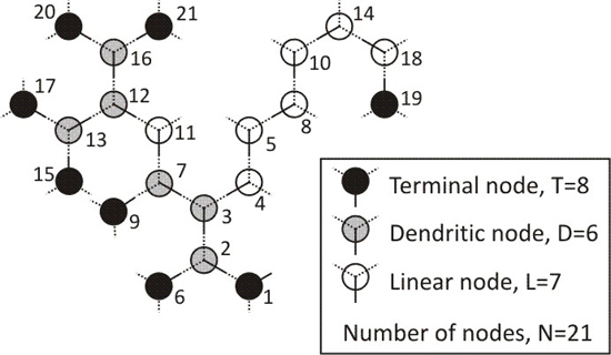
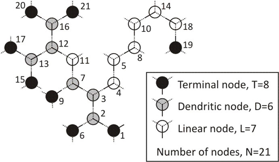
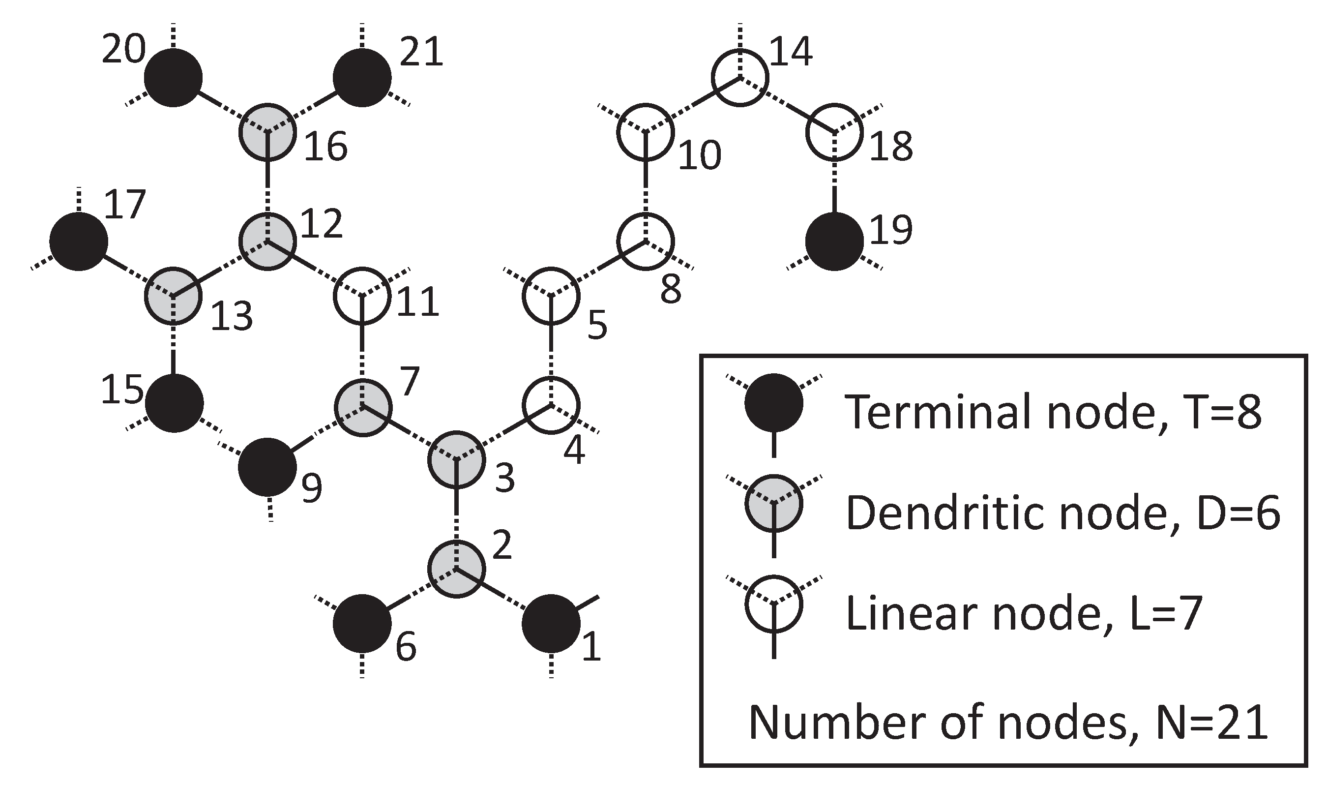
2.1. Topology

Any polymer chain without cyclic structures made of N nodes will contain N − 1 connectors. The maximum connectivity of a node is called the node functionality, F. According to F, the nodes can be classified into three types:

(1)

End or terminal nodes (T ) if they are connected to just 1 other node,

(2)

Linear nodes (L) if they are connected to 2 other nodes, and

(3)

Branching or dendritic nodes (D) if they are connected to f nodes, being f any number from 3 to F.

If T , L and D indicate the number of terminal, linear and dendritic nodes, respectively, the total number of nodes in a given polymer chain will be N = T + L + D.

The polymers studied in this work are formed by AB₂ monomers. That type of monomer is commonly used to build hyperbranched structures and has two types of reactive groups: A and B. The molecule grows by addition of the group A of one monomer to one free group B of other monomer with the subsequent emergence of a new free group B in the structure. Those AB₂ monomers correspond to nodes of functionality F = 3 so that every dendritic node in the structure must be connected to three other nodes (i.e., f = 3). A sketch of a hyperbranched polymer with N = 21 nodes made of AB₂ monomers is depicted in Figure 2. For the sake of clarity, T, L and D nodes are represented by different colors and numbered from 1 to 21, and groups A and B in each node are distinguished with solid and dotted lines respectively.

Figure 2. Sketch of a possible AB₂ hyperbranched structure with N = 21 nodes.

Figure 2. Sketch of a possible AB₂ hyperbranched structure with N = 21 nodes.

2.1.1. Degree of Branching

In this work, we define the degree of branching as the ratio between the number of branches actually existing in the molecule, R, and its maximum possible value, R_max: DB = R/R_max [12]. As commented above, for the particular case of an AB₂ type hyperbranched chain there is only one type of dendritic node with f = 3. Since linear and terminal nodes do not contribute to R and each dendritic node increments R in 1, then R = D. As a consequence, R_max will be the maximum number of dendritic nodes, D_max, that can exist in a structure with N nodes and, therefore, DB = R/R_max = D/D_max. It can be shown that D_max = int[(N − 2)/2] where “int” stands for the integer ratio. If N is large D_max ≈ N/2, and DB ≈ 2D/N = 2D/(T + L + D). An almost equivalent expression is DB ≈ 2D/(2D + L) [12], which can be derived from our argumentation considering that D ≈ T for AB₂ structures (indeed D = T − 2 counting the initial node as L or T according to its connectivity).

2.1.2. Generation of Chain Topology

Since a flexible hyperbranched polymer does not have a regular branched structure, the polymer properties must be calculated as averages over both different conformations of a given topology and different topologies. We generate AB₂ type chains with different topology by randomly attaching a new node to an existing node which has one or two free positions (i.e., free B groups). In order to control the degree of branching during the chain generation, we define the “attachment probability parameter” p. That parameter quantifies how much likely is for a node with one free position to incorporate the new node in comparison to a node with two free positions. For the latter p = 1 so that the probability of generating a highly branching structure (i.e., DB → 1) increases as p is greater than 1. The value p = 0 generates exclusively linear structures whereas any other p value can generate different branching structures with different (albeit generally similar) DB values. In spite of that DB uncertainty, one can establish a general relation between p and an average degree of branching 〈DB〉. Thus, we found the relationship 〈DB〉 = (p² + 0.35p)/(p² + 1.06p + 0.02) to fit quite well the dependence of 〈DB〉 on p for any number of nodes N . That 〈DB〉 vs. p relationship is useful to determine the p value that must be employed in order to generate chains with a certain DB value.

We do not have experimental DB values for the polymers studied in this work except for PDHBI whose authors report DB = 0.5 ± 0.1 [21]. Therefore, we decided to generate the four hyperbranched polymers studied here by setting p = 0.425 which provides an average degree of branching 〈DB〉 = 0.54 ± 0.04 that we consider representative of many real hyperbranched polymers.

2.2. Coarse-Grained Model

The model that will be ultimately used for the prediction of the solution properties of the hyperbranched polymer is a bead-and-spring model. Each bead represents an AB₂ monomer and is connected with other beads by linear springs that capture the connectivity. Thus, the model contains N beads or nodes and N − 1 springs as appreciated in Figure 2. The linear springs are defined by a potential devised in our previous work [15] that is an hybrid of Fraenkel (hard Hookean) and FENE (finitely extensible, non-linear elastic) springs [26]. As an elastic connector representing a chemical entity, the spring must have an equilibrium length l_e and a Hookean spring constant H_HF that gauges the fluctuation of the instantaneous length l. In addition, in order to account for the limited extensibility of the branches, the potential includes a maximum length, l_max. All the features of our “hard-FENE” springs are represented by the equation:

$$V_{conn}\left(l\right)=-\frac{1}{2}{H}_{HF}{l}_{\mathit{max}}^2\ln \left(1-\frac{l^2}{l_{\mathit{max}}^2}\right)-\frac{1}{2}{H}_{HF}{l}_{\mathit{max}}{l}_e\ln \left(\frac{l_{\mathit{max}}+l}{l_{\mathit{max}}-l}\right)$$

(1)

The conformational freedom at the branching points has restrictions that are represented by angular springs with the following simple quadratic potential:

$$V_{ang}\left(\theta \right)=\frac{1}{2}Q{\left(\theta -{\theta }_0\right)}^2$$

(2)

where θ is the supplementary angle to the bond angle (θ = 0 for aligned connectors), θ₀ is the equilibrium angle, and Q is the bending constant.

We must also include excluded volume (EV) interactions between nonbonded beads. For the sake of the simplicity that inspires our model, the EV effect is represented by a purely repulsive hard sphere (HS) potential: if the distance between two nonbonded beads is less or equal than the contact distance, σ_HS, the potential value becomes infinity (in practice a sufficiently high value), and otherwise the potential value is zero. The calculation of hydrodynamic properties requires the assignment of a hydrodynamic (Stokes) radius to the beads, a. Again, with the intention of maximum simplicity we have decided that this radius would also be the hard-sphere radius for the EV effect, so that σ_HS = 2a.

Thus, the set of values of a, l_e, H_HF, l_max, Q, and θ₀ defines completely the mechanical (conformational and dynamic) behavior of our coarse-grained model of the hyperbranched polymer.

2.3. Monte Carlo Simulation and Hydrodynamics

The prediction of both conformational and hydrodynamic properties for our flexible models is performed by using the rigid-body Monte Carlo procedure (RBMC) [27,28,29]. In the RBMC procedure, the properties are evaluated as means of the calculated values for each conformation in the Monte Carlo sample, as if the conformation were instantaneously rigid. We have used our public-domain program MONTEHYDRO [24] (available at: http://leonardo.inf.um.es/macromol/programs/programs.htm) which carries out both the Monte Carlo generation of conformations and the calculation of individual and average values for a general bead-and-connector model of arbitrary topology.

The hydrodynamic calculation for an array of beads is feasible using standard bead modeling procedures. A particular difficulty in bead-model calculations has been that concerning the intrinsic viscosity. The hydrodynamic approach of Kirkwood and Riseman [30,31], on which bead-model methods are based, does not take into account the volume of the beads in the model, which may give rise to erroneous values of the intrinsic viscosity when the size of the beads are not much smaller than the size of the molecule modeled by them. An improved theory that considered this missing influence [32] arrived at the so-called volume correction for the intrinsic viscosity:

[η]corr = [η]uncorr + f_η(5N_AV/2M)

(3)

where N_A is the Avogadro’s number, M the molecular weight of the solute and V the volume of the bead model. In the original derivation f_η = 1 so that the correction is the Einsteinian viscosity of a sphere of the same volume as the model. In some preliminary predictions of the intrinsic viscosity Equation (3) was applied with full volume correction [33]. More recently an application of this correction to a variety of bead models [34] showed that while [η]uncorr (i.e., f_η = 0) is a lower-bound that always underestimates the correct value, the result with full volume correction [η]corr with f_η = 1 produces an upper-bound overestimation. Clearly, an intermediate correction with 0 < f_η < 1 would be more appropriate. With results gathered for such a collection of bead models, an empirical correlation has been determined between the optimum f_η and two features of the model, namely its asphericity and its degree of fragmentation. The present version of the hydrodynamic calculation routines inserted in MONTEHYDRO includes the determination of the optimum f_η and the corresponding volume correction.

2.4. Atomic-Level Calculations

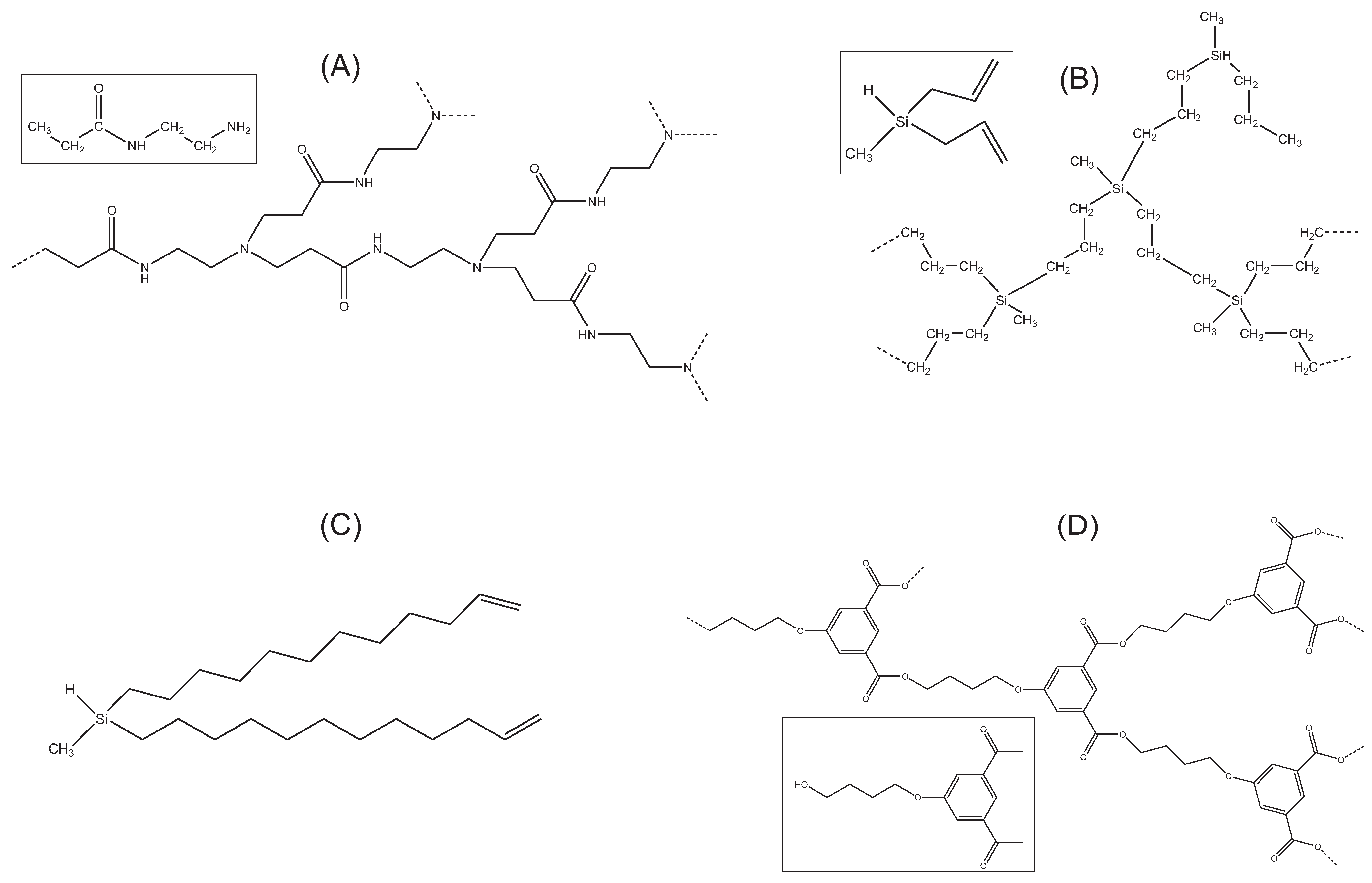
In our multi-scale approach the values of the coarse-grained model parameters corresponding to a given hyperbranched molecule are assigned from atomic-level Langevin molecular dynamics simulations of the minimum polymer fragment that contains the coarse-grained elements whose parameters are to be determined. Therefore, the model does not have free parameters to be fit to experimental data. The Langevin molecular dynamics simulations were carried out by using the commercial software HYPERCHEM (http://www.hyper.com) with the AMBER force field at T = 300 K. The simulation conditions were: time step ∆t = 0.001 ps, collision frequency 50 ps⁻¹, and duration of the trajectory about 100 ns. Under those conditions we found that simulations are well equilibrated and produce reproducible data.

• Beads:
  The atomic-level simulation with HYPERCHEM allows to sweep the conformational space of the monomeric unit represented by a bead. From the atomic coordinates, the hydrodynamic Stokes radius $R_h=\frac{f_t}{6\pi {\eta }_0}$ (where f_t is the friction coefficient of the particle and η₀ the solvent viscosity), and the equivalent radius to radius of gyration $R_G=\sqrt{\frac{5}{3}}{R}_g$, are computed for each conformation by using our public domain program HYDROPRO [22] (see http://leonardo.inf.um.es/macromol/programs/programs.htm). Regarding the possible influence of solvation on the effective hydrodynamic radius of the atoms, we follow previous experience [35] that, in the case of small molecular entities, such effective radius can be equated to the Van der Waals radius, of typically 1.8 Å [36]. The results are the averages over a sample of conformations. Because R_h turns out to be similar to R_G, we take as the hydrodynamic radius of the bead representing the monomer unit their mean a = (R_G + R_h)/2.
  In order to avoid free parameters in the model, the radius of the beads in the hard spheres EV potential was taken equal to a so that the contact distance becomes σ_HS = 2a. This choice seems convenient because it makes neighboring beads almost tangent and prevent “phantom” crosses of the connectors.
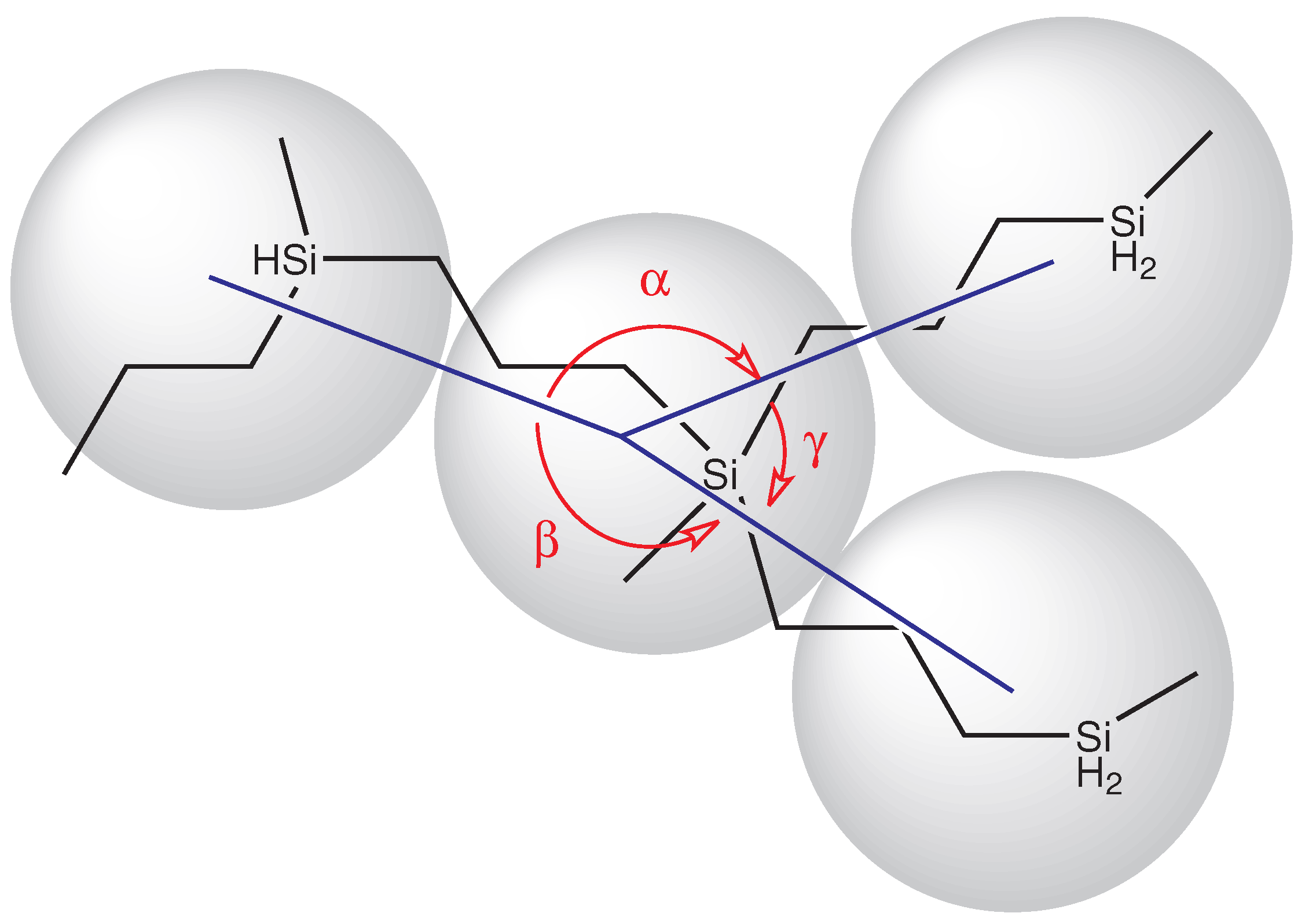
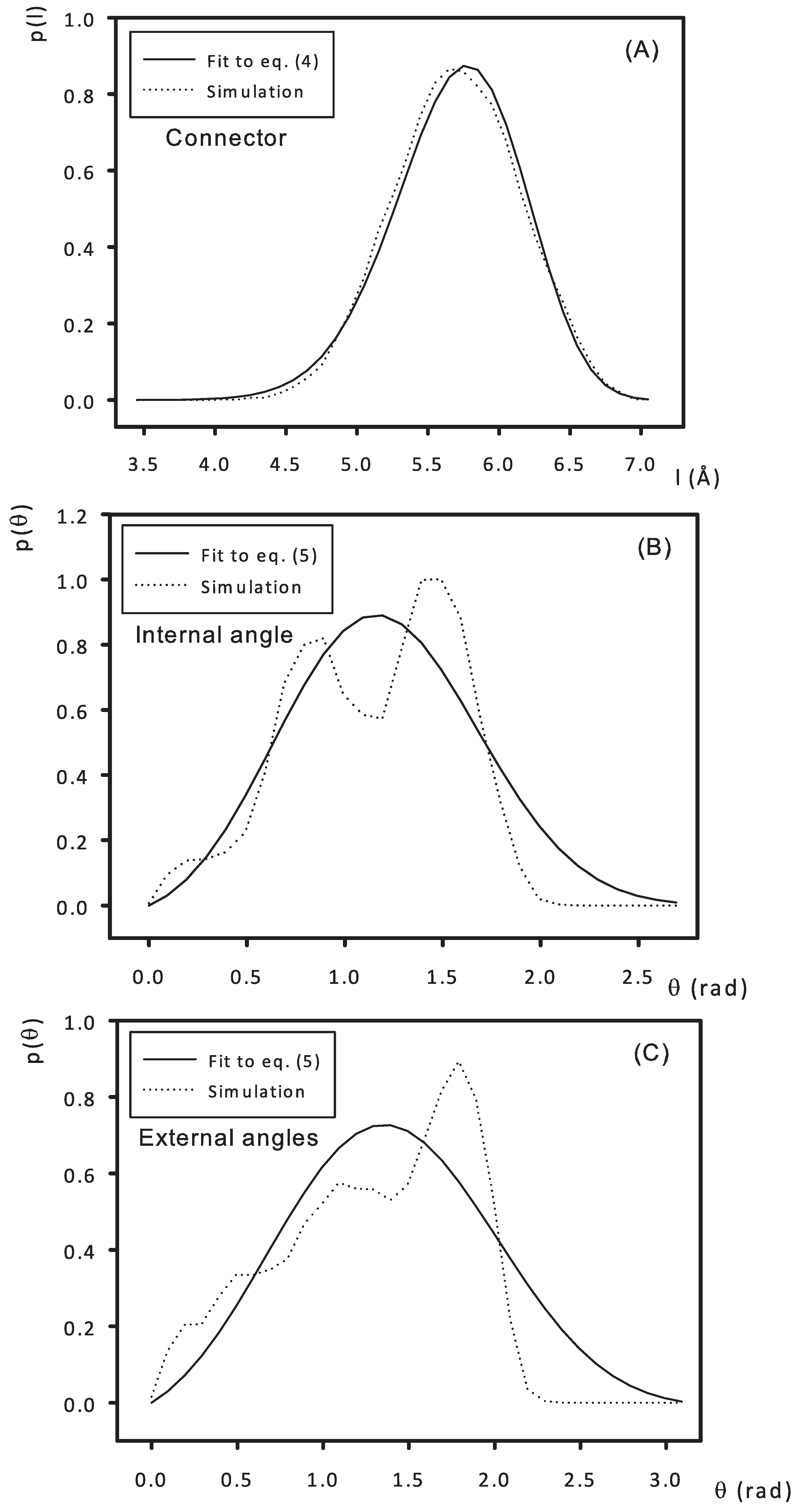
• Connector and angles:
  Parameters of the potentials associated to connectors and angles were estimated from atomic-level simulations of the minimal atomic structure that defines those connectors and angles, as illustrated in Figure 3 for a PCS3. From the atomic trajectories generated with program HYPERCHEM, the distribution functions for connector length (taken as the distance between the centers of mass of two connected monomers/beads) and the angle subtended by those connectors were obtained.
  We distinguish between two types of angles: “internal” angles subtended between the two B groups of a monomer and “external” angles subtended between the groups A and B of the monomer (see Figure 3). In terms of the formation process of the bead-and-connector model, the “internal” angle is that subtended between the two free connectors emerging from a newly incorporated node, and the “external” angle is that subtended between any one of those free connectors and the connector that links that new node to the chain structure. Then, the connector length distribution and the two angles distributions were fit, respectively, to the Boltzmann exponentials associated to the connector-spring potential and the angle-spring potentials (see Figure 4):

  p(l) = A_ll² exp[−V(l)/k_BT]

  (4)

  p(θ) = A_θ sinθ exp[−V (θ)/k_BT]

  (5)

  where A_l and A_θ are normalization constants.

In that way, we obtained the values of the coarse-grained parameters that best fit the atomic-level distributions for the four studied hyperbranched polymers: PAMAM, PCS3, PCS11 and PDHBI. As an example, we comment the results obtained for the parameterization of PCS3. The HYDROPRO result for the bead radius is a = 4.5 Å. The atomic-level simulation yields the distribution functions for the connector length and inter-connector angles shown in Figure 4. The fit of the simulated p(l) to the Boltzmann exponential associated to Equations (1) and (4) gives H_HF = 1131 erg/cm², l_max = 9.1 Å, and l_e = 5.7 Å. On the other hand, the fit of the simulated p(θ) to Equations (2) and (5) gives Q = 1.1 × 10⁻¹³ erg and θ₀ = 1.0 rad for the supplementary “internal” angle (being γ in Figure 3 the “internal” angle) as well as Q = 5.7 × 10⁻¹⁴ erg and θ₀ = 1.2 rad for the supplementary “external” angles (being α and β in Figure 3 the “external” angles). In Figure 4, the fitted Boltzmann exponentials are plotted along with the original distribution functions coming from the atomic-level simulations. We remark that the fits do not reproduce the details of the simulated distribution functions–as it corresponds to a coarse-grained representation of the true potentials–but provide continuous potential functions that are conveniently handled in the Monte Carlo simulations of the coarse grained model.

Figure 3. Atomic structure of the PCS3 monomer, showing the beads, connectors and angles.

Figure 3. Atomic structure of the PCS3 monomer, showing the beads, connectors and angles.

Figure 4. Distribution of (A) connector length; (B) “internal” angle; and (C) “external” angles in the branches of PCS3. Results from the atomic-level Langevin simulation and their best fits to Equations (1) and (2).

Figure 4. Distribution of (A) connector length; (B) “internal” angle; and (C) “external” angles in the branches of PCS3. Results from the atomic-level Langevin simulation and their best fits to Equations (1) and (2).

3. Results and Discussion

We have studied how the polymer properties R_g, D_t, and [η] vary with the molecular weight (which would be a mean molecular weight in the real polydisperse samples). For that purpose, we have simulated for each case (PAMAM, PCS3, PCS11 and PDHBI), coarse-grained models containing from N = 50 to N = 400 beads/nodes. Since each node represents a monomer, the molecular weight corresponding to each N will be calculated as the monomer molecular weight times the number of nodes. On the other hand, for a given N we have run 600 independent simulations varying slightly the topology of the chain so that polymer properties are computed as both a conformational average and a topological average. Nevertheless, it must be remarked that the topological variability may be insufficient since the parameter p is fixed (p = 0.425) what produces only small variations in DB. Moreover, for the sake of simplicity, the polydispersity of the sample is not actually considered (for instance, generating chains with different molecular weight by a reaction kinetic method [37]). Thus, all of the chains used to perform the 600 simulations corresponding to a given mean molecular weight are indeed of the same length N (instead of N being an average) so that the sample is treated as monodisperse.

The radius of gyration R_g gives a direct measurement of the mean molecular size. Figure 5 is a log–log plot that represents the variation of R_g with the molecular weight, M, for the hyperbranched polymers studied in this work. We do not compare with experiments because we do not have experimental R_g data for most of the polymers studied here. In a first approximation, all of the cases can be fit to linear plots which gives rise to the typical power law of linear flexible polymers R_g ∝ M^α_g, where α_g is the slope of the plots in Figure 5. However, the values of those slopes is generally smaller than the characteristic value of the random coil conformation of flexible linear polymers in theta solvent (i.e., 0.5). In particular, we found the following slope values: α_g (PAMAM) ≈ 0.19, α_g (PCS3) ≈ 0.32, α_g (PCS11) ≈ 0.38, and α_g (PDHBI) ≈ 0.51. It must be noticed that PDHBI has the largest branches and is the most flexible among the polymers studied here so that it is expected to present a random coil conformation with a value of the power law exponent about 0.5 (as for linear flexible polymers). It is also interesting to notice that a value of α_g ≈ 0.35 was found in our previous work for dendrimers [15] as well as g in some other simulations with dendrimers [38]. Thus, hyperbranched polymers seem to behave in some aspects similarly to dendrimers; obviously, the similarities will be more remarkable in increasing the degree of branching. The value α_g = 1/3 is the theoretical expectation for spherical particles of uniform density whereas for flexible/semiflexible non-spherical structures α_g should be larger than 1/3. Nonetheless, the increase in R_g with M can be smaller than it should be for spheres of constant density if some backfolding effect is present. It means that terminal branches tend to get back to the polymer core (the initial monomer) so that the effective volume, proportional to $R_g^3$, grows slower than M and the exponent of R_g vs. M is smaller than 1/3. That effect must become more remarkable with increasing the degree of branching of the polymer and therefore the number of terminal nodes.

As indicated above, from our simulations we have also predicted (in a multi-scale approach, without adjustable parameters) two hydrodynamic overall solution properties for which some experimental data are available: the diffusion coefficient D_t and the intrinsic viscosity [η], being the latter the most frequently reported hydrodynamic property. In order to compare simulation and experimental D_t values, it is convenient to work in terms of the equivalent hydrodynamic Stokes radius, R_h, because it is solvent and temperature independent (and our simulation conditions are not always coincident with experiments). We compute the characteristic polymer Stokes radius from the D_t value by using the Stokes-Einstein relationship D_t = k_BT/(6πη₀R_h), where k_BT is the Boltzmann factor and η₀ is the solvent viscosity. On the other hand, the intrinsic viscosity coming from our simulations can be directly compared to experimental data.

Figure 5. Double-log plots of the radius of gyration of the four hyperbranched polymers vs. molecular weight.

Figure 5. Double-log plots of the radius of gyration of the four hyperbranched polymers vs. molecular weight.

Concerning [η], it does not increase, in general, monotonically with the molecular weight and cannot be fit to a power law (a linear relation in a log-log plot) as it is common for linear flexible polymers. In some cases, [η] even reaches a maximum value and then keeps constant or decreases, a behavior often found in dendrimer solutions [15]. As commented above, for high enough DB the effective (hydrodynamic) volume of the molecule may grow with M (or N ) less than expected due to the backfolding effect what explains that particular [η] behavior.

Figure 6 is a log–log plot showing the comparison of our simulation results for the intrinsic viscosity (empty circles) with experimental data [18] (black circles) for PAMAM. Both set of data display the same trend: firstly [η] increases slightly, then reaches a maximum and finally tends to decrease. However, our simulation results yield [η] values clearly higher than the experimental ones. Likewise, our maximum is shifted to a higher molecular weight. The lack of good correspondence between the topological variability and polydispersity of the real polymer and our simplified model may be an important source of discrepancy in the solution properties values.

Figure 7A,B shows the comparison between our simulation results and experimental data [19,20] for the variation of [η] and R_h with the molecular weight for the polymer PCS3. Semi-log plots are used in order to better appreciate the non-monotonic molecular weight dependence and the differences between experimental and simulation values. Again, simulation results overestimate the experimental values. The type of dependency of [η] with the molecular weight is quite similar in both simulation and experimental results. On the other hand, R_h values from simulations seem to diverge from the few available experimental data. Figure 8A,B is the analogous to Figure 7 for PCS11 [20]. For that polymer, the values of [η] coming from simulations reproduce reasonable well the experimental data. Concerning R_h, the discrepancy between simulation and experimental data is about 50%, although molecular weight dependences are qualitatively similar. For this long-branched polymer the simulation values are smaller than the experimental ones.

Finally, Figure 9A,B displays our results for the polymer PDHBI along with the experimental ones [21] in terms of semi-log plots representing the molecular weight dependence of [η] and R_h. Again, the simulation results underestimate experimental values in about 50%.

It is interesting to notice that simulations results for hyperbranched polymers with small and relatively stiff monomers (PAMAM and PCS3) overestimate the experimental values whereas simulations for those polymers whose monomers contains larger branches (PCS11 and PDHBI) underestimate the experimental values. On the other hand, the hyperbranched polymer with shorter and stiffer branches (PAMAM) exhibit an intrinsic viscosity behavior similar to that of dendrimers (with a maximum in the molecular weight dependence of [η]) whereas those hyperbranched polymers with long branches (PCS11 and PDHBI) tend to behave as linear flexible polymers (monotonic increase of [η] with the molecular weight that would eventually lead to a power law). Therefore, the larger the branches the closer the hyperbranched polymer to a linear polymer. Notice how [η] for the short-branched PCS3 polymer increases with M at a smaller rate than [η] for its long-branched counterpart PCS11. Obviously, it must be also true that the greater the degree of branching of the hyperbranched polymer the more similar its behavior to that of a dendrimer, although such a point was not tested because all of the cases studied in this work correspond to a same degree of branching (〈DB〉 = 0.54 ± 0.04).

Figure 6. Variation of the intrinsic viscosity with the molecular weight for PAMAM. Comparison of simulation and experimental results.

Figure 6. Variation of the intrinsic viscosity with the molecular weight for PAMAM. Comparison of simulation and experimental results.

Figure 7. Variation of (A) the intrinsic viscosity and (B) the hydrodynamic radius with the molecular weight for PCS3. Comparison of simulation and experimental results.

Figure 7. Variation of (A) the intrinsic viscosity and (B) the hydrodynamic radius with the molecular weight for PCS3. Comparison of simulation and experimental results.

The main conclusion is that our multi-scale simulations without adjustable parameters are able to qualitatively reproduce the experimental behavior but not yet fully capable of reproducing the hydrodynamic properties of these hyperbranched molecules accurately. Therefore, our procedure must be improved in order to obtain quantitative agreement between simulations and experiments. On the other hand, it is clear that the high variability in the degree of polymerization and the degree of branching of the hyperbranched polymers generates an important uncertainty in the determination of their properties values. Thus, experimental data must be affected by errors (not reported in the original works) that should be consider to better quantify the differences with our simulations results.

Figure 8. Variation of (A) the intrinsic viscosity and (B) the hydrodynamic radius with the molecular weight for PCS11. Comparison of simulation and experimental results.

Figure 8. Variation of (A) the intrinsic viscosity and (B) the hydrodynamic radius with the molecular weight for PCS11. Comparison of simulation and experimental results.

Figure 9. Variation of (A) the intrinsic viscosity and (B) the hydrodynamic radius with the molecular weight for PDHBI. Comparison of simulation and experimental results.

Figure 9. Variation of (A) the intrinsic viscosity and (B) the hydrodynamic radius with the molecular weight for PDHBI. Comparison of simulation and experimental results.

4. Conclusions

In this work, we have implemented a scheme for the prediction of properties of hyperbranched polymers using a very simple coarse-grained model whose parameters are not adjusted to fit experimental data. Instead they are obtained, in a multi-scale approach, from previous atomic-level simulations which are also done in a simple fashion with Langevin dynamics of small pieces of the molecules. The procedure predicts conformational and hydrodynamic properties of the four studied hyperbranched polymers which differ from experimental data typically in about 50%, although simulation results tend to reproduce qualitatively the dependency of the properties with the molecular weight. Obviously, the double source of polydispersity (degree of polymerization and degree of branching) makes our simple multi-scale procedure not yet appropriate for quantitative predictions of hydrodynamic properties of hyperbranched polymers, in spite of its excellent performance for the prediction of solution properties of regular monodisperse dendrimers (where the typical difference respect to experimental data was found to be about 4% [15]).

A possible reason for the quantitative disagreement between experimental and simulation results is the poor statistical representativity, both in terms of polydispersity and topological variability, of the samples used in our simulations. Thus, the number of different degree of polymerization and topologies (for a given degree of polymerization) that can appear in a one-pot reaction are surely much higher than the ones taken into account in our simulations. This explanation is specially plausible if one considers the excellent results obtained in our previous works with monodisperse polymers of well defined topology [15,16,17]. Apart from it, the average degree of branching about 0.5 assumed to carry out our simulations may be not the correct one for all of the polymers.

Obviously, improvements must be performed in both the parameterization and mainly the ensemble generation procedures in order our methodology to be applicable to obtain quantitative predictions of hyperbranched polymers properties in solution. Still, the present scheme opens the possibility to understand and predict single-molecular behavior of hyperbranched structures from first principles without resorting to free adjustable parameters. In the present work, the coarse-grained model has been simulated by a Monte Carlo procedure to obtain overall conformational and hydrodynamic properties of the molecule. The same model (with the forces derived from the analytical potentials) could be used in Brownian dynamics simulations in order to study dynamic aspects that would be out of reach of fully atomic-level molecular dynamics simulations.

References

1. Seiler, M. Hyperbranched polymers: Phase behavior and new applications in the field of chemical engineering. Fluid Phase Equilib. 2006, 241, 155–174. [Google Scholar] [CrossRef]
2. Hawker, C.J.; Fréchet, J.M.J. Control of surface functionality in the synthesis of dendritic macromolecules using the convergent-growth approach. Macromolecules 1990, 23, 4726–4729. [Google Scholar] [CrossRef]
3. Flory, P.J. Molecular size distribution in three dimensional polymers. VI. Branched polymers containing A–R–Bf−1 type units. J. Am. Chem. Soc. 1952, 74, 2718–2723. [Google Scholar] [CrossRef]
4. Zhang, B.; Yu, H.; Schlüter, A.D.; Halperin, A.; Kröger, M. Synthetic regimes due to packing constraints in dendritic molecules confirmed by labelling experiments. Nat. Commun. 2013, 4. [Google Scholar] [CrossRef]
5. Kröger, M.; Schlüter, A.D.; Halperin, A. Branching defects in dendritic molecules: Coupling efficiency and congestion effects. Macromolecules 2013, 46, 7550–7564. [Google Scholar] [CrossRef]
6. Aerts, J. Prediction of intrinsic viscosities of dendritic, hyperbranched and branched polymers. Comput. Theor. Polym. Sci. 1998, 8, 49–54. [Google Scholar] [CrossRef]
7. Widmann, A.H.; Davies, G.R. Simulation of the intrinsic viscosity of hyperbranched polymers built by sequential addition. Comput. Theor. Polym. Sci. 1998, 8, 191–199. [Google Scholar] [CrossRef]
8. Lyulin, A.V.; Adolf, D.B.; Davies, G.R. Computer simulations of hyperbranched polymers in shear flows. Macromolecules 2001, 31, 3783–3789. [Google Scholar] [CrossRef]
9. Sheridan, P.F.; Adolf, D.B.; Lyulin, A.V.; Neelov, I.; Davies, G.R. Computer simulations of hyperbranched polymers: The influence of the Wiener index on the intrinsic viscosity and radius of gyration. J. Chem. Phys. 2002, 117, 7802–7812. [Google Scholar] [CrossRef]
10. Mulder, T.; Lyulin, A.V.; van der Schoot, P.; Michels, M.A.J. Architecture and conformation of uncharged and charged hyperbranched polymers: Computer simulation and mean-field theory. Macromolecules 2005, 38, 996–1006. [Google Scholar] [CrossRef]
11. Wiener, H. Structural determination of paraffin boiling points. J. Am. Chem. Soc. 1947, 69, 17–20. [Google Scholar] [CrossRef] [PubMed]
12. Hölter, D.; Burgath, A.; Frey, H. Degree of branching in hyperbranched polymers. Acta Polym. 1997, 48, 30–35. [Google Scholar] [CrossRef]
13. Del Río Echenique, G.; Hernández Cifre, J.G.; Rodríguez, E.; Rubio, A.; Freire, J.J.; García de la Torre, J. Multi-scale simulation of the conformation and dynamics of dendrimeric macromolecules. Chem. Macromol. Symp. 2007, 245, 386–389. [Google Scholar]
14. Freire, J.J. Realistic numeric simulations of dendrimer molecules. Soft Matter 2008, 4, 2139–2143. [Google Scholar] [CrossRef]
15. Del Río Echenique, G.; Rodríguez Schmidt, R.; Freire, J.J.; Hernández Cifre, J.G.; García de la Torre, J. A multiscale scheme for the simulation of conformational and solution properties of different dendrimer molecules. J. Am. Chem. Soc. 2009, 131, 8548–8556. [Google Scholar] [CrossRef] [PubMed]
16. Rodríguez Schmidt, R.; Pamies, R.; Kjøniksen, A.L.; Zhu, K.; Hernández Cifre, J.G.; Nyström, B.; García de la Torre, J. Single-molecule behavior of asymmetric thermoresponsive amphiphilic copolymers in dilute solution. J. Phys. Chem. B 2010, 114, 8887–8893. [Google Scholar] [CrossRef] [PubMed]
17. Maleki, A.; Zhu, K.; Pamies, R.; Rodríguez Schmidt, R.; Kjøniksen, A.L.; Karlsson, G.; Hernández Cifre, J.G.; García de la Torre, J.; Nyström, B. Effect of polyethylene Glycol (PEG) length on the association properties of temperature-sensitive amphiphilic triblock copolymers (PNIPAAMm-b-PEGn-b-PNIPAAMm) in aqueous solution. Soft Matter 2011, 7, 8111–8119. [Google Scholar] [CrossRef]
18. Hobson, L.J.; Feast, W.J. Poly(amidoamine) hyperbranched systems: Synthesis, structure and characterization. Polymer 1999, 40, 1279–1297. [Google Scholar] [CrossRef]
19. Tarabukina, E.B.; Shpyrkov, A.A.; Potapova, D.V.; Filippov, A.P.; Shumilkina, N.A.; Muzafarov, A.M. Hydrodynamic and conformational properties of a hyperbranched polymethylallylcarbosilane in dilute solutions. Polym. Sci. Ser. A 2006, 48, 974–980. [Google Scholar] [CrossRef]
20. Tarabukina, E.B.; Shpyrkov, A.A.; Tarasova, E.V.; Amirova, A.I.; Filippov, A.P.; Sheremet’eva, N.A.; Muzafarov, A.M. Effect of the length of branches on hydrodynamic and conformational properties of hyperbranched polycarbosilanes. Polym. Sci. Ser. A 2009, 51, 150–160. [Google Scholar] [CrossRef]
21. De Luca, E.; Richards, R.W. Molecular characterization of a hyperbranched polyester. I. Dilute solution properties. J. Polym. Sci. B 2003, 41, 1339–1351. [Google Scholar] [CrossRef]
22. García de la Torre, J.; Huertas, M.L.; Carrasco, B. Calculation of hydrodynamic properties of globular proteins from their atomic-level structures. Biophys. J. 2000, 78, 719–730. [Google Scholar] [CrossRef] [PubMed]
23. García de la Torre, J.; Pérez Sánchez, H.E.; Ortega, A.; Hernández Cifre, J.G.; Fernandes, M.X.; Díaz Baños, F.G.; López Martínez, M.C. Calculation of the solution properties of flexible macromolecules: Methods and applications. Eur. Biophys. J. 2003, 32, 477–486. [Google Scholar] [CrossRef] [PubMed]
24. García de la Torre, J.; Ortega, A.; Pérez Sánchez, H.E.; Hernández Cifre, J.G. MULTIHYDRO and MONTEHYDRO: Conformational search and Monte Carlo calculation of solution properties of rigid and flexible macromolecular models. Biophys. Chem. 2005, 116, 121–128. [Google Scholar] [CrossRef] [PubMed]
25. Lu, Y.; An, L.; Wang, Z.-G. Intrinsic viscosity of polymers: General theory based on partially permeable sphere model. Macromolecules 2013, 46, 5731–5740. [Google Scholar] [CrossRef]
26. Bird, R.B.; Curtiss, C.F.; Armstrong, R.C.; Hassager, O. Dynamics of Polymeric Liquids, Kinetic Theory, 2nd ed.; John Wiley and Sons: New York, NY, USA, 1987; Volume 2. [Google Scholar]
27. Zimm, B.H. Chain molecule hydrodynamics by the Monte-Carlo method and the validity of the Kirkwood–Riseman approximation. Macromolecules 1980, 13, 592–602. [Google Scholar] [CrossRef]
28. García de la Torre, J.; Jiménez, A.; Freire, J.J. Monte Carlo calculation of hydrodynamic properties of freely jointed, freely rotating and real polymethylene chains. Macromolecules 1982, 15, 148–154. [Google Scholar] [CrossRef]
29. García de la Torre, J.; Freire, J.J. Intrinsic viscosities and translational diffusion coefficients of n-alkanes in solution. Macromolecules 1982, 15, 155–159. [Google Scholar] [CrossRef]
30. Kirkwood, J.G.; Riseman, J. The intrinsic viscosities and diffusion constants of flexible macromolecules in solution. J. Chem. Phys. 1948, 16, 565–573. [Google Scholar] [CrossRef]
31. Kirkwood, J.G. The general theory of irreversible processes in solutions of macromolecules. J. Polym. Sci. 1954, 12, 1–14. [Google Scholar] [CrossRef]
32. Carrasco, B.; Garcia de la Torre, J. Intrinsic viscosity and rotational diffusion of bead models for rigid macromolecules and bioparticles. Eur. Biophys. J. 1998, 27, 549–557. [Google Scholar] [CrossRef]
33. Rodríguez, E.; Freire, J.J.; Del Río Echenique, G.; Hernández Cifre, J.G.; García de la Torre, J. Improved simulation method for the calculation of the intrinsic viscosity of some dendrimer molecules. Polymer 2007, 48, 1155–1163. [Google Scholar] [CrossRef]
34. García de la Torre, J.; del Río Echenique, G.; Ortega, A. Improved calculation of rotational diffusion and intrinsic viscosity of bead models for macromolecules and nanoparticles. J. Phys. Chem. B 2007, 111, 955–961. [Google Scholar] [CrossRef] [PubMed]
35. Espinosa, P.; García de la Torre, J. Theoretical prediction of translational diffusion coefficients of small rigid molecules. J. Phys. Chem. 1987, 91, 3612–3616. [Google Scholar] [CrossRef]
36. Bondi, A. Van der Waals volumes and radii. J. Phys. Chem. 1964, 68, 441–451. [Google Scholar] [CrossRef]
37. Wang, L.; He, X. Investigation of ABn (n = 2, 4) type hyperbranched polymerization with cyclization and steric factors: Influences of monomer concentration, reactivity, and substitution effect. J. Polym. Sci. Pol. Chem. 2009, 47, 523–533. [Google Scholar] [CrossRef]
38. Karatasos, K.; Adolf, D.B.; Davies, G.R. Statics and dynamics of model dendrimers as studied by molecular dynamics simulations. J. Chem. Phys. 2001, 115, 5310–5318. [Google Scholar] [CrossRef]