
Developed Hybrid Model for Propylene Polymerisation at Optimum Reaction Conditions


Abstract
:
1. Introduction
2. Experimental Study
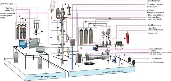
2.1. Description of Experimental Setup


2.2. Measurement and Analysis System
2.3. Model Development for Optimisation

| Code of the factor | Factor name | Units | Type | Low coded | High coded | Low actual | High actual |
|---|---|---|---|---|---|---|---|
| A | Reaction temperature (RT) | °C | Numeric | −1.000 | 1.000 | 70.00 | 80.00 |
| B | System pressure (SP) | bar | Numeric | −1.000 | 1.000 | 20.00 | 30.00 |
| C | Monomer concentration (MC) | % | Numeric | −1.000 | 1.000 | 70.00 | 80.00 |
| Physical properties | Value | ||||||
| Bubble diameter (m) | 550 × 10−4 | ||||||
| Gas velocity (m/s) | 0.50 | ||||||
| Gas density (kg/m3) | 23.45 | ||||||
| Gas viscosity (Pa s) | 1.14 × 10⁻⁴ | ||||||
| Polymer density (kg/m3) | 1000 | ||||||
| Void fraction of the bed at minimum fluidisation | 0.45 | ||||||
2.3.1. CFD Modelling of Gas-Solid Phenomenon in FBCR
2.3.2. Phase Sequestration
| Parameter | Formula | Reference |
|---|---|---|
| Bubble velocity | [36] | |
| Bubble rise velocity | [37] | |
| Emulsion velocity | [38] | |
| Bubble diameter | (Geldard B category) | [39] |
| Bubble phase fraction | [40] | |
| Emulsion phase porosity | [40] | |
| Bubble phase porosity | [40] | |
| Volume of polymer phase in the emulsion phase | [17] | |
| Volume of polymer phase in the bubble phase | [31] | |
| Volume of the emulsion phase | [41] | |
| Volume of the bubble phase | [37] | |
| Minimum fluidisation velocity | [37] | |
| Mass transfer coefficient | [20] | |
| Momentum exchange coefficient | [12] |
2.3.3. Mass Balance Model
2.3.4. Conservation of Momentum
- the default algebraic equation based on Equation (16), which disregards any diffusion and convection in transport;
- a partial equation of the differential based on Equation (16), which uses various property options;
- the constant value of the granular temperature which can be applied in the cases of small arbitrary variations;
2.3.5. Solids Pressure
3. Results and Discussion
| Run | Factor A RT (°C) | Factor B SP (bar) | Factor CMC (%) | Response, Yppc, (%) (Actual) |
|---|---|---|---|---|
| 1 | 70 | 25 | 75 | 5.96 |
| 2 | 70 | 25 | 75 | 4.83 |
| 3 | 70 | 20 | 70 | 4.53 |
| 4 | 80 | 30 | 70 | 5.10 |
| 5 | 75 | 20 | 75 | 5.90 |
| 6 | 70 | 30 | 70 | 4.57 |
| 7 | 75 | 25 | 70 | 5.62 |
| 8 | 75 | 25 | 75 | 5.98 |
| 9 | 75 | 25 | 80 | 5.94 |
| 10 | 70 | 20 | 80 | 5.63 |
| 11 | 75 | 25 | 75 | 5.96 |
| 12 | 75 | 25 | 75 | 5.97 |
| 13 | 75 | 25 | 75 | 5.95 |
| 14 | 80 | 25 | 75 | 5.89 |
| 15 | 70 | 30 | 80 | 5.53 |
| 16 | 75 | 25 | 75 | 5.95 |
| 17 | 75 | 30 | 75 | 5.92 |
| 18 | 80 | 30 | 80 | 5.95 |
| 19 | 80 | 20 | 70 | 4.98 |
| 20 | 80 | 20 | 80 | 5.93 |
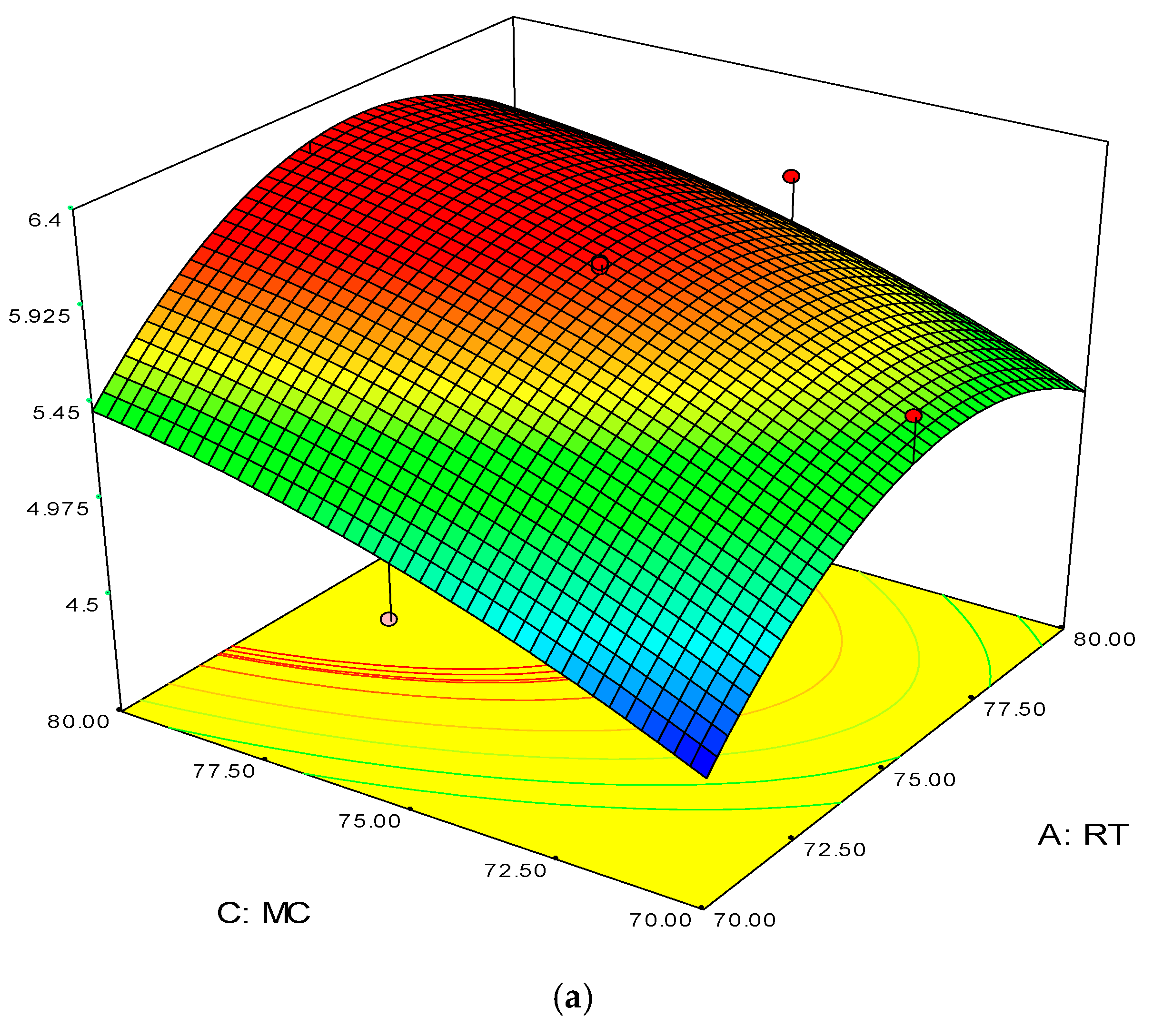
3.1. RSM Analysis


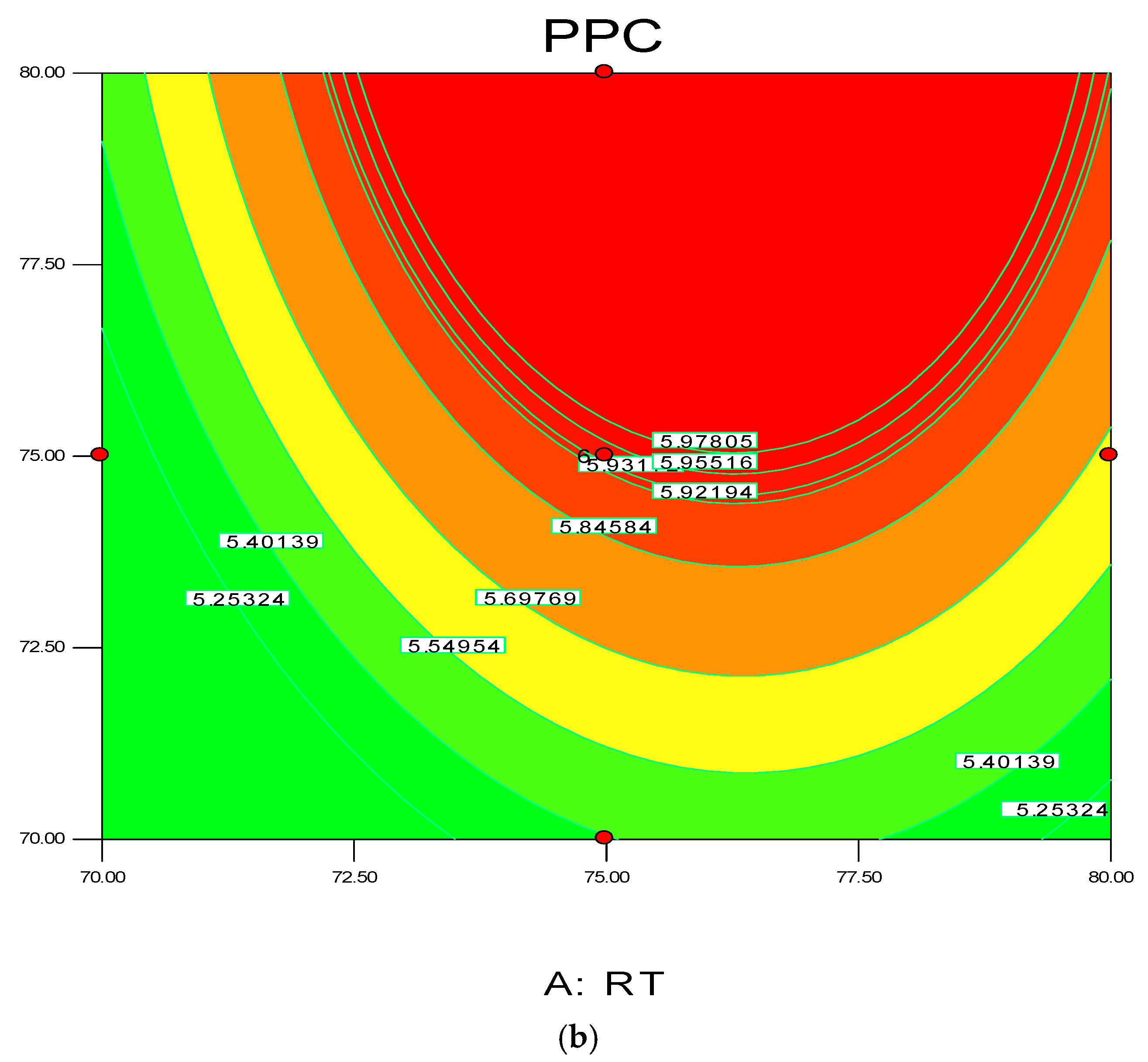
3.2. Effect of Process Conditions on Bed Structure during Reaction
3.2.1. Boundary Conditions
| Factors | Value | |
|---|---|---|
| Reaction zone | Inner diameter | 0.1016 m |
| Cross sectional area | 0.00785 m2 | |
| Height | 1.5 m | |
| Volume | 0.011775 m3 | |
| Disengagement zone | Inner diameter | 0.25 m |
| Cross sectional area | 0.0490625 m2 | |
| Height | 0.25 m | |
| Volume | 0.0097 m3 | |
| Reactor volume | 0.0215 m3 | |
| Initial bed height (m) | 1.5 | |
| Initial void fraction | 0.431 | |
| Gas density (kg/m3) | 23.45 | |
| Gas viscosity (Pa·s) | 1.14 × 10⁻⁴ | |
| Particle density (kg/m3) | 910 | |
| Coefficient of restitution | 0.8 | |
| Angle of internal fraction | 30 | |
| Maximum solid packing volume fraction | 0.75 | |
| Time step (s) | 0.001 | |
| Activation energy, E (J·mol−1) | 7.04 × 10⁴ | |
| Active site of catalyst (mol·m−3) | 1.88 × 10⁻⁴ | |
| Feed monomer concentration (mol·m−3) | 0.75 | |
| Pre-exponential factor, kp0 (m3·mol−1·s−1) | 1.2 × 10⁴ | |
3.2.2. Model Validation and Grid Sensitivity Analysis
3.2.3. Grid Independent Analysis


3.2.4. Fluidized Bed Dynamics at Various Set of Process Conditions

3.3. Examining the Model Accuracy


3.3.1. Interaction Graphs


3.3.2. Perturbation Graph

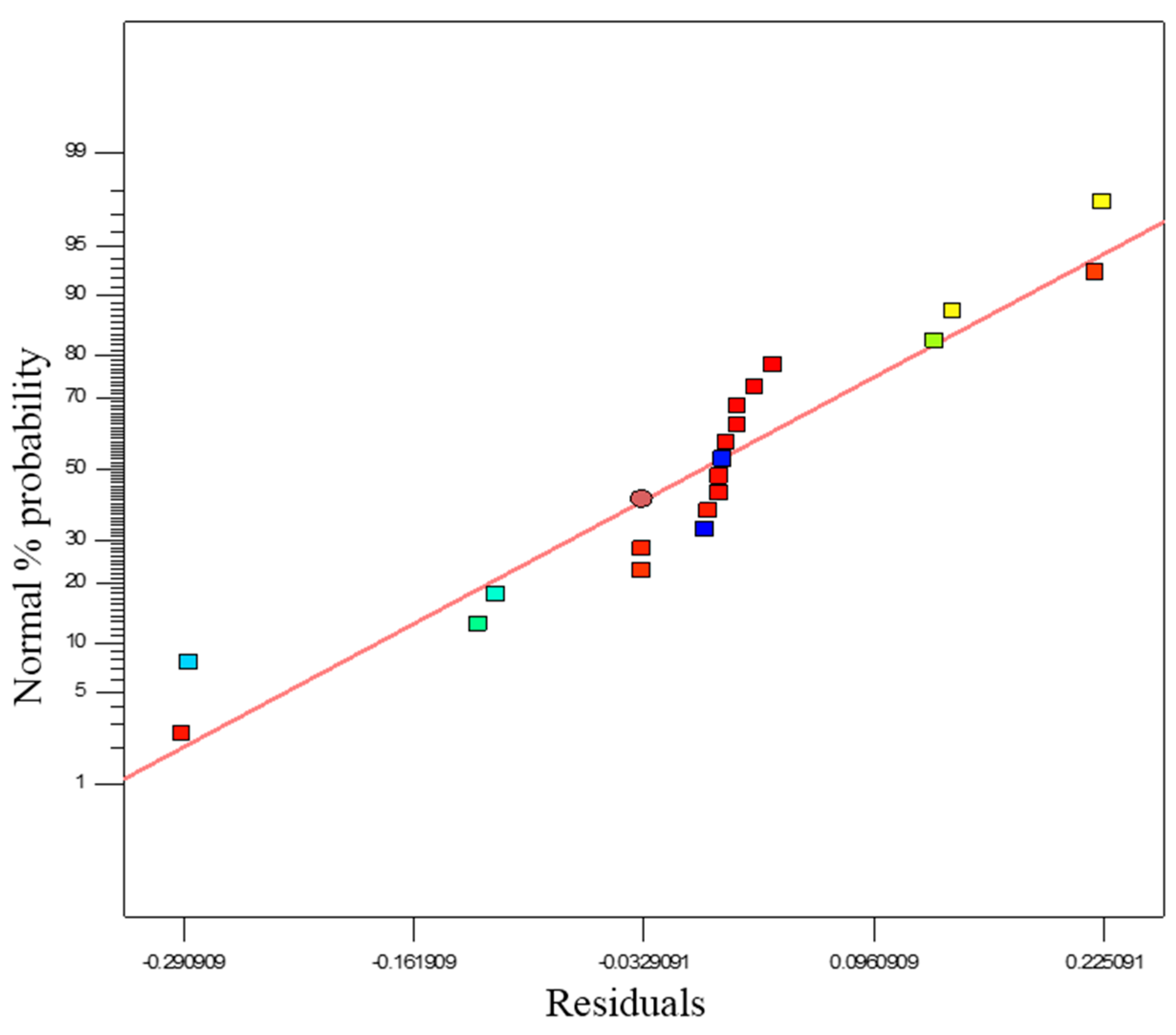
3.4. Statistical Diagnosis of the Model through ANNOVA Analysis
| Functions | Degree of freedom,df | Mean Square | F-Value | p-Value (Prob > F) |
|---|---|---|---|---|
| Model | 9 | 0.57 | 14.80 | <0.0001 |
| A-RT | 1 | 0.76 | 22.50 | 0.0008 |
| B-SP | 1 | 0.003 | 0.006 | 0.867 |
| C-MC | 1 | 1.75 | 51.62 | <0.0001 |
| A2 | 1 | 0.82 | 24.29 | 0.0006 |
| B2 | 1 | 0.009 | 0.018 | <0.9777 |
| C2 | 1 | 0.044 | 1.31 | <0.2796 |
4. Financial Benefits
5. Conclusions
Supplementary Materials
Acknowledgments
Author Contributions
Conflicts of Interest
Notations
| A | Cross-sectional area of the reactor (m2) |
| Ar | Archimedes number |
| ANOVA | Analysis of variance |
| DgFmod | Degree of freedom of mode |
| DgFresidual | Degree of freedom of residual |
| F-value | Model significance |
| H | Bed height (m) |
| MnSer | Mean Square Error |
| MnSRD | Mean of square residual |
| MnSRG | Mean of square regression |
| N | Number of experiments |
| P | Number of model parameters |
| p | Pressure shared by all phases |
| Pmw | Propylene molecular weight (kg/kmol) |
| PPC | Polypropylene Concentration |
| Prt | Rate of propylene consumption |
| R2 | Determination coefficient |
| R2adj | Adjusted coefficient of determination |
| SD | Standard deviation |
| SRD | Sum of residual |
| SRG | Sum of squares |
| SSQ | Sum of squares |
| SSQmod | Sum of squares of model |
| SSQresidual | Sum of squares of residual |
| v0 | Superficial gas velocity (m/s) |
| vmf | Minimum fluidisation velocity (m/s) |
| Yp | Predicted value |
| YR | Response yield |
| Ε | Error vector |
| ω2 | Residual value |
| db | Bubble diameter (m) |
| Void fraction of the bed at minimum fluidisation | |
| Velocity of gas phase | |
| Mass transfer from the solid to gas phase | |
| Mass transfer from the gas to solid phase | |
| Velocity of solid phase | |
| Shear viscosity of gas phase | |
| Bulk viscosity of gas phase | |
| External body force for gases | |
| Lift force for gas phase | |
| Virtual mass force for gas phase | |
| Interaction force between solid–gas phases | |
| Interphase solid to gas velocity |
References
- Arencón, D.; Velasco, J.I. Fracture toughness of polypropylene-based particulate composites. Materials 2009, 2, 2046–2094. [Google Scholar] [CrossRef] [Green Version]
- Tian, Z.; Xue-Ping, G.; Feng, L.-F.; Guo-Hua, H. A model for the structures of impact polypropylene copolymers produced by an atmosphere-switching polymerization process. Chem. Eng. Sci. 2013, 101, 686–698. [Google Scholar] [CrossRef]
- Delva, L.; Ragaert, K.; Degrieck, J.; Cardon, L. The effect of multiple extrusions on the properties of montmorillonite filled polypropylene. Polymers 2014, 6, 2912–2927. [Google Scholar] [CrossRef] [Green Version]
- Galli, P.; Vecellio, G. Polyolefins: The most promising large-volume materials for the 21st century. J. Polym. Sci. Polym. Chem. 2004, 42, 396–415. [Google Scholar] [CrossRef]
- Nguyen, T.-A.; Gregersen, Ø.; Männle, F. Thermal oxidation of polyolefins by mild pro-oxidant additives based on iron carboxylates and lipophilic amines: Degradability in the absence of light and effect on the adhesion to paperboard. Polymers 2015, 7, 1522–1540. [Google Scholar] [CrossRef]
- Bikiaris, D. Microstructure and properties of polypropylene/carbon nanotube nanocomposites. Materials 2010, 3, 2884–2946. [Google Scholar] [CrossRef]
- Umair, S.; Numada, M.; Amin, M.; Meguro, K. Fiber reinforced polymer and polypropylene composite retrofitting technique for masonry structures. Polymers 2015, 7, 963–984. [Google Scholar] [CrossRef]
- Pracella, M.; Haque, M.M.-U.; Alvarez, V. Functionalization, compatibilization and properties of polyolefin composites with natural fibers. Polymers 2010, 2, 554–574. [Google Scholar] [CrossRef]
- Glauß, B.; Steinmann, W.; Walter, S.; Beckers, M.; Seide, G.; Gries, T.; Roth, G. Spinnability and characteristics of polyvinylidene fluoride (PVDF)-based bicomponent fibers with a carbon nanotube (CNT) modified polypropylene core for piezoelectric applications. Materials 2013, 6, 2642–2661. [Google Scholar] [CrossRef] [Green Version]
- Hisayuki, N.; Dodik, K.; Toshiaki, T.; Minoru, T. Degradation behavior of polymer blend of isotactic polypropylenes with and without unsaturated chain end group. Sci. Technol. Adv. Mater. 2008, 9, 1–6. [Google Scholar]
- Balow, M.J. Handbook of Polypropylene and Polypropylene Composites; CRC Press: New York, NY, USA, 2003. [Google Scholar]
- Syamlal, M.; Rogers, W.; O’Brien, T.J. Mfix Documentation: Theory Guide; National Energy Technology Laboratory, U.S. Department of Energy: Morgantown, WV, USA, 1993. [Google Scholar]
- Gharibshahi, R.; Jafari, A.; Haghtalab, A.; Karambeigi, M.S. Application of CFD to evaluate the pore morphology effect on nanofluid flooding for enhanced oil recovery. RSC Adv. 2015, 5, 28938–28949. [Google Scholar] [CrossRef]
- McAuley, K.B.; Talbot, J.P.; Harris, T.J. A comparison of two-phase and well-mixed models for fluidized-bed polyethylene reactors. Chem. Eng. Sci. 1994, 49, 2035–2045. [Google Scholar] [CrossRef]
- Jarullah, A.T.; Mujtaba, I.M.; Wood, A.S. Kinetic parameter estimation and simulation of trickle-bed reactor for hydrodesulfurization of crude oil. Chem. Eng. Sci. 2011, 66, 859–871. [Google Scholar] [CrossRef]
- Ahmadzadeh, A.; Arastoopour, H.; Teymour, F.; Strumendo, M. Population balance equations’ application in rotating fluidized bed polymerization reactor. Chem. Eng. Res. Des. 2008, 86, 329–343. [Google Scholar] [CrossRef]
- Shamiri, A.; Azlan Hussain, M.; Sabri Mjalli, F.; Mostoufi, N.; Saleh Shafeeyan, M. Dynamic modeling of gas phase propylene homopolymerization in fluidized bed reactors. Chem. Eng. Sci. 2011, 66, 1189–1199. [Google Scholar] [CrossRef]
- Kaushal, P.; Abedi, J. A simplified model for biomass pyrolysis in a fluidized bed reactor. J. Ind. Eng. Chem. 2010, 16, 748–755. [Google Scholar] [CrossRef]
- Jang, H.T.; Park, T.S.; Cha, W.S. Mixing-segregation phenomena of binary system in a fluidized bed. J. Ind. Eng. Chem. 2010, 16, 390–394. [Google Scholar] [CrossRef]
- Ibrehem, A.S.; Hussain, M.A.; Ghasem, N.M. Modified mathematical model for gas phase olefin polymerization in fluidized-bed catalytic reactor. Chem. Eng. J. 2009, 149, 353–362. [Google Scholar] [CrossRef]
- Jarullah, A.T.; Mujtaba, I.M.; Wood, A.S. Improving fuel quality by whole crude oil hydrotreating: A kinetic model for hydrodeasphaltenization in a trickle bed reactor. Appl. Energy 2012, 94, 182–191. [Google Scholar] [CrossRef]
- Khan, M.; Hussain, M.; Mujtaba, I. Polypropylene production optimization in fluidized bed catalytic reactor (FBCR): Statistical modeling and pilot scale experimental validation. Materials 2014, 7, 2440–2458. [Google Scholar] [CrossRef]
- Yahya, A.M.; Hussain, M.A.; Abdul Wahab, A.K. Modeling, optimization, and control of microbial electrolysis cells in a fed-batch reactor for production of renewable biohydrogen gas. Int. J. Energy Res. 2015, 39, 557–572. [Google Scholar] [CrossRef]
- Özer, A.; Gürbüz, G.; Çalimli, A.; Körbahti, B.K. Biosorption of copper(II) ions on enteromorpha prolifera: Application of response surface methodology (RSM). Chem. Eng. J. 2009, 146, 377–387. [Google Scholar] [CrossRef]
- Sridhar, V.; Prasad, K.; Choe, S.; Kundu, P.P. Optimization of physical and mechanical properties of rubber compounds by a response surface methodological approach. J. Appl. Polym. Sci. 2001, 82, 997–1005. [Google Scholar] [CrossRef]
- Shamiri, A.; Hussain, M.A.; Mjalli, F.S.; Mostoufi, N. Improved single phase modeling of propylene polymerization in a fluidized bed reactor. Comput. Chem. Eng. 2012, 36, 35–47. [Google Scholar] [CrossRef]
- Shamiri, A.; Hussain, M.A.; Mjalli, F.S.; Mostoufi, N. Kinetic modeling of propylene homopolymerization in a gas-phase fluidized-bed reactor. Chem. Eng. J. 2010, 161, 240–249. [Google Scholar] [CrossRef]
- Armstrong, L.M.; Luo, K.H.; Gu, S. Two-dimensional and three-dimensional computational studies of hydrodynamics in the transition from bubbling to circulating fluidised bed. Chem. Eng. J. 2010, 160, 239–248. [Google Scholar] [CrossRef]
- Li, Z.; van Sint Annaland, M.; Kuipers, J.A.M.; Deen, N.G. Effect of superficial gas velocity on the particle temperature distribution in a fluidized bed with heat production. Chem. Eng. Sci. 2016, 140, 279–290. [Google Scholar] [CrossRef]
- Che, Y.; Tian, Z.; Liu, Z.; Zhang, R.; Gao, Y.; Zou, E.; Wang, S.; Liu, B. Cfd prediction of scale-up effect on the hydrodynamic behaviors of a pilot-plant fluidized bed reactor and preliminary exploration of its application for non-pelletizing polyethylene process. Powder Technol. 2015, 278, 94–110. [Google Scholar] [CrossRef]
- Akbari, V.; Borhani, T.N.G.; Godini, H.R.; Hamid, M.K.A. Model-based analysis of the impact of the distributor on the hydrodynamic performance of industrial polydisperse gas phase fluidized bed polymerization reactors. Powder Technol. 2014, 267, 398–411. [Google Scholar] [CrossRef]
- Bi, H.T.; Grace, J.R. Flow regime diagrams for gas-solid fluidization and upward transport. Int. J. Multiphase Flow 1995, 21, 1229–1236. [Google Scholar] [CrossRef]
- Xie, N.; Battaglia, F.; Pannala, S. Effects of using two- versus three-dimensional computational modeling of fluidized beds: Part I, hydrodynamics. Powder Technol. 2008, 182, 1–13. [Google Scholar] [CrossRef]
- Alchikh-Sulaiman, B.; Ein-Mozaffari, F.; Lohi, A. Evaluation of poly-disperse solid particles mixing in a slant cone mixer using discrete element method. Chem. Eng. Res. Design 2015, 96, 196–213. [Google Scholar] [CrossRef]
- Xie, N.; Battaglia, F.; Pannala, S. Effects of using two- versus three-dimensional computational modeling of fluidized beds: Part II, budget analysis. Powder Technol. 2008, 182, 14–24. [Google Scholar] [CrossRef]
- Lucas, A.; Arnaldos, J.; Casal, J.; Puigjaner, L. Improved equation for the calculation of minimum fluidization velocity. Indust. Eng. Chem. Process Design Dev. 1986, 25, 426–429. [Google Scholar] [CrossRef]
- Kunii, D.L.O. Fluidization Engineering, 2nd ed.; Butterworth-Heinmann: Boston, MA, USA, 1991. [Google Scholar]
- Mostoufi, N.; Cui, H.; Chaouki, J. A comparison of two- and single-phase models for fluidized-bed reactors. Ind. Eng. Chem. Res. 2001, 40, 5526–5532. [Google Scholar] [CrossRef]
- Silva, E.L. Hydrodynamics characteristics and gas-liquid mass transfer in a three phase fluidized bed reactor. J. Braz. Soc. Mech. Sci. 2001, 23, 503–512. [Google Scholar] [CrossRef]
- Cui, H.; Mostoufi, N.; Chaouki, J. Characterization of dynamic gas–solid distribution in fluidized beds. Chem. Eng. J. 2000, 79, 133–143. [Google Scholar] [CrossRef]
- Wang, S.; Zhao, Y.; Li, X.; Liu, L.; Wei, L.; Liu, Y.; Gao, J. Study of hydrodynamic characteristics of particles in liquid–solid fluidized bed with modified drag model based on emms. Adv. Powder Technol. 2014, 25, 1103–1110. [Google Scholar] [CrossRef]
- Batchelor, G.K. An Introduction to Fluid Dynamics; Cambridge University Press: Cambridge, UK, 1967. [Google Scholar]
- Gidaspow, D.; Bezburuah, R.; Ding, J. Hydrodynamics of Circulating Fluidized Beds: Kinetic Theory Approach. In Proceedings of the 7th international conference on fluidization, Gold Coast, Australia, 3–8 May 1992.
- Van Wachem, B.; Schouten, J.; Krishna, R.; van den Bleek, C. Eulerian simulations of bubbling behaviour in gas–solid fluidised beds. Comp. Chem. Eng. 1998, 22, S299–S306. [Google Scholar] [CrossRef]
- Dompazis, G.; Kanellopoulos, V.; Touloupides, V.; Kiparissides, C. Development of a multi-scale, multi-phase, multi-zone dynamic model for the prediction of particle segregation in catalytic olefin polymerization fbrs. Chem. Eng. Sci. 2008, 63, 4735–4753. [Google Scholar] [CrossRef]
- Chen, W.-J.; Su, W.-T.; Hsu, H.-Y. Continuous flow electrocoagulation for msg wastewater treatment using polymer coagulants via mixture-process design and response-surface methods. J. Taiwan Inst. Chem. Eng. 2012, 43, 246–255. [Google Scholar] [CrossRef]
- Thouchprasitchai, N.; Luengnaruemitchai, A.; Pongstabodee, S. Statistical optimization by response surface methodology for water-gas shift reaction in a h2-rich stream over Cu–Zn–Fe composite-oxide catalysts. J. Taiwan Inst. Chem. Eng. 2011, 42, 632–639. [Google Scholar] [CrossRef]
- Harshe, Y.M.; Utikar, R.P.; Ranade, V.V. A computational model for predicting particle size distribution and performance of fluidized bed polypropylene reactor. Chem. Eng. Sci. 2004, 59, 5145–5156. [Google Scholar] [CrossRef]
- Sidorenko, I.; Rhodes, M.J. Influence of pressure on fluidization properties. Powder Technol. 2004, 141, 137–154. [Google Scholar] [CrossRef]
- Rietema, K.; Piepers, H.W. The effect of interparticle forces on the stability of gas-fluidized beds—I. Experimental evidence. Chem. Eng. Sci. 1990, 45, 1627–1639. [Google Scholar] [CrossRef]
- Norouzi, H.R.; Mostoufi, N.; Mansourpour, Z.; Sotudeh-Gharebagh, R.; Chaouki, J. Characterization of solids mixing patterns in bubbling fluidized beds. Chem. Eng. Res. Design 2011, 89, 817–826. [Google Scholar] [CrossRef]
- Petrochemical Plants at Gebeng. Available online: http://www.petronas.com.my/our-business/downstream/petro-chemicals/gebeng-ipc/Pages/gebeng-ipc/petrochemical-plants-gebeng.aspx (accessed on 3 January 2016).
- GPCA PLASTICON 2016—Global Polypropylene Demand to Rise 5%/year up to 2020: GPCA. Available online: http://www.platts.com/latest-news/petrochemicals/asia/gpca-plasticon-2016---global-polypropylene-demand-26336697 (accessed on 14 January 2016).
© 2016 by the authors. Licensee MDPI, Basel, Switzerland. This article is an open access article distributed under the terms and conditions of the Creative Commons by Attribution (CC-BY) license ( http://creativecommons.org/licenses/by/4.0/).
Share and Cite
Khan, M.J.H.; Hussain, M.A.; Mujtaba, I.M. Developed Hybrid Model for Propylene Polymerisation at Optimum Reaction Conditions. Polymers 2016, 8, 47. https://doi.org/10.3390/polym8020047
Khan MJH, Hussain MA, Mujtaba IM. Developed Hybrid Model for Propylene Polymerisation at Optimum Reaction Conditions. Polymers. 2016; 8(2):47. https://doi.org/10.3390/polym8020047
Chicago/Turabian StyleKhan, Mohammad Jakir Hossain, Mohd Azlan Hussain, and Iqbal Mohammed Mujtaba. 2016. "Developed Hybrid Model for Propylene Polymerisation at Optimum Reaction Conditions" Polymers 8, no. 2: 47. https://doi.org/10.3390/polym8020047