Abstract
Canopy characteristics are crucial for accurately and safely determining the pesticide quantity and volume of water used for spray applications in vineyards. The inevitably high degree of intraplot variability makes it difficult to develop a global solution for the optimal volume application rate. Here, the design procedure of, and the results obtained from, a variable rate application (VRA) sprayer are presented. Prescription maps were generated after detailed canopy characterization, using a multispectral camera embedded on an unmanned aerial vehicle, throughout the entire growing season in Torrelavit (Barcelona) in four vineyard plots of Chardonnay (2.35 ha), Merlot (2.97 ha), and Cabernet Sauvignonn (4.67 ha). The maps were obtained by merging multispectral images with information provided by DOSAVIÑA®, a decision support system, to determine the optimal volume rate. They were then uploaded to the VRA prototype, obtaining actual variable application maps after the application processes were complete. The prototype had an adequate spray distribution quality, with coverage values in the range of 20–40% and exhibited similar results in terms of biological efficacy on powdery mildew compared to conventional (and constant) application volumes. The VRA results demonstrated an accurate and reasonable pesticide distribution, with potential for reduced disease damage even in cases with reduced amounts of plant protection products and water.
1. Introduction
Pesticide spray application is one of the most important factors that influences all economic, environmental, and quality-related aspects of worldwide vineyard operations. Vineyards, with their grape-bearing vines and their relationship with wine production, are one of the crop-types of focus among the recently named “specialty crops” [1]. Several challenges exist when considering improvements in the application process. The Mediterranean zone in particular requires further training and education, taking into account its specific characteristics.
The application of pesticides requires accuracy, as imprecise or excessive use can lead to serious problems such as environmental pollution, traces of pesticides in food, and health issues in humans; both workers and bystanders [2]. During the application process, risk, as a function of pesticide dose and harm to sensitive non-target areas, is related to (a) the spraying efficiency and (b) the amount of plant protection products (PPPs) used during the distribution process across the entire canopy. For orchard and vineyard applications, however, the various methods used to determine the most suitable amount of PPP and the corresponding application volume rate are often difficult to understand [3].
It is suggested that accurately determining the spray rate based on the canopy structure can improve the quality of pesticide application, resulting in better pest/disease control and reduced risk of contamination. This could also lead to reduced amounts of pesticide used, which brings consequential economic, environmental, and social benefits. However, not all trees and bush crops have the same structure and uniformity, and in some cases, it is difficult to characterize the geometric parameters of the intended target. Moreover, canopy characterization could vary from very simple measurements of the main structural parameters (e.g., canopy height, canopy width) down to the most sophisticated, detailed aspects (e.g., leaf area density, porosity, leaf area index). A significant amount of previous research has demonstrated the clear influence of the canopy structure and dimensions on the success of the spray application process [4,5,6,7,8,9,10]. These studies have established a clear necessity to determine the optimal amount of pesticide to be used based on the canopy characteristics, as opposed to determining the amount by simply quantifying the ground surface area.
Accurate canopy characterization is often linked with the promising concept of variable rate pesticide application. Assuming that the objective is to maintain a constant application rate per unit of canopy, developments regarding canopy measurement methods have been linked with research into modified sprayers. Using these, various spray parameters (working pressure, nozzle flow rate, number of nozzles, etc.) can be modified according to the canopy characteristics, while maintaining a constant application rate per unit of canopy [11,12,13].
Canopy characterization then becomes a crucial aspect within site-specific management strategies. In particular, when georeferenced information regarding the canopy structure and variability at the field scale is required [14], the use of non-destructive remote sensing technologies becomes a promising option. These technologies make rapid assessment of large areas possible [15,16]. Unmanned Aerial Vehicles (UAVs) have been widely utilized to carry remote sensing devices due their versatility, flexibility regarding flight scheduling and affordable management. Using this technology, spatial information linked, both directly and indirectly, with canopy characteristics or information about designed areas can be recorded in a practical and efficient way. Examples of this information include water status [17], disease detection [18] and canopy characterization [19,20,21,22]. De Castro et al. developed a fully automatic process for vineyard canopy characterization [14], which self-adapts to varying crop conditions. This represents an important improvement in the canopy characterization process, generating a time efficient, reliable, and accurate method, in addition to avoiding potential errors inherent to the manual process.
Recent research has demonstrated interest in the use of UAVs for canopy characterization and the potential improvements to the application process considering the intra-parcel variability [14,23]. This inherent variability, especially in large parcel situations, has led to increased interest in the development of advanced sprayers that could modify the spray application parameters in order to adapt the amount of PPP to the canopy structure. The European Directive on Sustainable Use of Pesticides highlighted this as an important step in reducing the risk of pesticide use [24], through facilitating a reduction in the applied dose per hectare, improving the deposition quality and controlling the environmental contamination risk.
Benefits of the implementation of variable application rate based on the intra-parcel variability have been demonstrated, not only by the potential reduction of applied PPP, but also for the more rational and logical distribution of the required dose, considering the pest/disease pressure and its negative effects on the crop development [15].
Vogel et al. evaluated a modified conventional boom sprayer for variable application of herbicide based on prescription maps [25]. The system was capable of combating weeds of corn and soybean crops. Furthermore, Michaud and coworkers developed a variable application prototype based on maps [26], obtained from aerial spectral images, to combat weeds in a cranberry crop. While variable rate application technology based on prescription maps is widely used in field crops, it is not used in 3D crops. For this reason, this research aims to develop a variable rate application (VRA) system, for vineyard sprayers, based on canopy vigor maps obtained with remote sensors.
Applying the latest technologies in crop protection process improvements to vineyards, arguably one of the most specialty crops in the Mediterranean zone, could massively benefit from this important and specific agriculture. Vineyards have been identified as agricultures with one of the lowest rates of adoption or implementation of precision farming, with a primary reason being the low educational level of their farmers [27,28]. Research progress in this topic, and increased use of new technologies, will lead to a more uniform educational level across all EU zones. A similar trend has been witnessed in recent years in field crop spraying [29].
The main objective of this research was to develop, and evaluate, a holistic and automatic process for large-scale variable rate application in commercial parcels of vineyard, considering the intra-parcel variability. The specific objectives of this work were as follows:
- Development of canopy variable maps using information acquired by specific remote sensing.
- Establishment of a protocol to transform canopy maps into PPP prescription maps;
- Implementation of the corresponding hardware and software on a commercial sprayer to enable georeferenced variable spray application according the developed prescription maps;
- Quantification of the benefits of the developed prototype in the global context of spray application.
2. Materials and Methods
This section presents the entire process carried out to implement the variable application rate in real conditions. This process follows the method of Campos et al. [23] and is summarized in Figure 1. The following steps can be distinguished: (1) Generation of canopy vigor map from UAV data; (2) generation of prescription maps for variable spray application based on canopy maps; (3) development of software and hardware to adapt a conventional sprayer into a Variable Rate Application (VRA) sprayer; and (4) generation of actual application rate map and monitoring of the results.
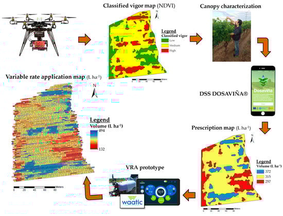
Figure 1.
Overview of the entire process used to implement the variable application rate in the field tests.
In order to assess the suitability of the developed VRA, parcels with conventional—and therefore constant—rate application were also included in this research and used as a reference.
2.1. Experimental Site
The trials were carried out on the Alt Penedès region (Torrelavid, Barcelona); an important wine production zone in the northeast of Spain. Seven different vineyards were selected, containing three representative varieties: Chardonnay, Merlot and Cabernet Sauvignon (Figure 2).
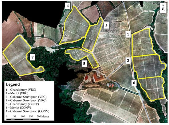
Figure 2.
Orthophoto map of the experimental vineyard parcels.
All of the selected vineyards were trained in a trellis system; Double Royat with 1.2 m on the row and 2.2 m between rows. Four of the selected parcels were sprayed with VRA system and the remaining three were sprayed using a conventional sprayer (CONV). The main characteristics of the selected vineyards are shown in Table 1.

Table 1.
Main characteristics of the vineyard parcels.
2.2. Generation of Canopy Vigor Maps
In order to obtain a complete range of data across the entire season, the vineyards were overflown with an unmanned aerial vehicle (UAV) at three different canopy stages. The first flight was scheduled on May 9th 2018, at BBCH around 57–60 [30]; the second flight was executed on June 11st (BBCH 69–75); and the third flight was performed on July 2nd (BBCH 77–79). A DroneHEXA (Dronetools SL, Sevilla, Spain) was used for the data acquisition. The UAV was equipped with two batteries of 6000 mAh (88.8 Wh), with a maximum autonomy of 25 min. The drone was loaded with a multispectral camera (RedEDGE, Micasense, Seattle, WA, USA) equipped with five spectral bands: 668 nm for Red with a bandwidth of 10 nm; 560 nm for Green with a bandwidth of 20 nm; 475 nm for Blue with a bandwidth of 20 nm; 717 nm for RedEdge with a bandwidth of 10 nm; and 840 nm for NIR with a bandwidth of 40 nm. Flights were conducted 95 m above ground level (AGL) at a cruise flight speed of 6 m s−1. Overlapping zones were adjusted at 80% in the sense of flight and 60% in the transverse sense.
In order to build the vigor map at each canopy stage, an orthophoto map with a ground sample distance (GSD) of 6.33 cm pixel−1 was obtained from spectral images acquired with the camera. The orthophoto map was radiometrically calibrated using four grayscale standards (22, 32, 44 and 51% grayscale reflectance), placed in the field during the flight, to transform grayscale 12-bit digital numbers to reflectance values. This new data were used to calculate the normalized differential vegetation index (NDVI) [31] (Equation (1)).
where NDVI is normalized difference vegetation index; NIR is reflection in the near-infrared spectrum; and RED is reflection in the red range of the spectrum.
As the vineyards were planted out in rows, the image was segmented by an NDVI threshold in order to eliminate weeds, shadows and soil occurring between rows. In each vigor map building process, different NDVI thresholds were established depending on the response of the not desired pixels (soil, shadows, weeds, etc.). The pixels above the set threshold were considered vineyard pixels and coded as “1”, whereas pixels below the set threshold were considered noise and set to “0”. Once the NDVI threshold was applied, an inverse distance weighting interpolation (IDW) was performed to generate a continuous NDVI map. Final processing consisted of value clustering in three NDVI levels, except in one case, where the clustering process only differentiated two NDVI levels due to the low intra-plot variability (Figure 3). In the case of three NDVI levels, the population were divided in quintiles (P20, P40, P60 and P80). The NDVI values lower than P20 were categorized as low vigor, values between P20 and P80 correspond to medium vigor and values higher than P80 were clustered into high vigor. P20 and P80 were selected as border lines to differentiate low and high vigor canopy zones, avoiding excessive weight to extreme zones. When only two NDVI levels were distinguished, the population were divided with the median (2-quantiles, P50). The NDVI values lower or equal than P50 corresponded to low vigor and those values higher than P50 were categorized as high vigor.
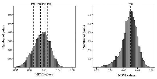
Figure 3.
Examples of histogram of the NDVI values for clustering in 3 (left) and 2 (right) vigor zones.
Finally, the latter data were smoothed by performing neighbor median filtering to produce the classified vigor map. The process was executed using QGIS software (OSGeo, Beaverton, OR, USA) [32].
2.3. Generation of Prescription Maps for Variable Spray Application
Once the vigor map was created, taking into account the different zones identified, it was located in the field using a GNSS receiver. In each determined vigor zone, 15 manual measurements of canopy height and width were randomly taken following EPPO standard [33]. After that, adjusted volume rates for every zone were determined using the decision support system (DSS) DOSAVIÑA® [3]. The values obtained using DOSAVIÑA® were introduced into the classified vigor map using QGIS software [32], in order to obtain the prescription map. This procedure was carried out for each pesticide application. Throughout the season, a total of seven pesticide applications were performed. This followed the experience and advice of the farmers’ experience, who recommended the adequate time taking into account the risk of pest/damage.
2.4. Adapted Sprayer for Variable Rate Application
A conventional trailed cross-flow air sprayer (Saher Maquinaria Agrícola S.L., Barcelona, Spain), with a 1000 L tank and an axial fan of 800 mm diameter, commonly used in vineyard regions, was adapted for variable pesticide application based on the prescription maps (VRA). To achieve this, the sprayer was equipped with: a) one pressure sensor—GEMS 1200 series (Gems Sensors & Controls, Plainville, CT, USA)—to allow working pressure to be monitored during the work; and b) an electronic controller—WAATIC (Estel Grup S.L., Barcelona, Spain)—including a GNSS receiver with a frequency of 1 Hz, a touchscreen and an automatic section controller. The purpose of the system was, firstly, to determine the position of the sprayer in the field as detected by the GNSS receiver. The system would then read the desired volume rate, based on the previously uploaded prescription map, and modify the working pressure using the electronic valve available in the conventional sprayer. This will then obtain the adjusted nozzle flow rate that is required to obtain the desired volume rate following Equation (2):
where q is the intended nozzle flow rate (l·min−1); a is working width (m); v is forward speed (km h−1)
Working pressure was automatically adjusted in the sprayer following Equation (3), established for every type of nozzle selected during the spray application process:
where p is the intended pressure (bar); q is the intended nozzle flow rate (l min−1); a and b are dimensionless coefficients depending on nozzle type and size.
Prior to each spray application, the prescription map, in GeoJSON format, was loaded via USB to the touch screen that was installed in the sprayer. Working parameters, such as the number and type of nozzles, as well as the working width, were also introduced into the system.
2.5. Generation of Actual Variable Rate Application Maps
Once spraying had commenced, the system recorded information concerning the sprayer position in the field, the applied volume rate and the adjusted working pressure, each second throughout operation. When spraying had finished, the system generated the actual variable rate application map, which was downloaded from the touch screen via USB. This methodology was repeated for every selected parcel and for every pesticide application process throughout the entire season.
2.6. Evaluation of the System Accuracy
In order to evaluate the accuracy of the system, the prescription maps and the actual variable rate application maps were compared following the methodology developed by Campos et al. [23], using QGIS software [32]. Within these comparison processes, a random net of 2 points m−2 was created, and each georeferenced random point was assigned with a prescript value “r” and an actual value “p”. For each prescript value “r”, 11 intervals of tolerance were assigned (from 0% to 50% deviation, increasing in steps of 5%). It was then determined if the actual value “p” was within the calculated range [r-i, r+i]. Once all the points were compared, the percentage of coincidence between the assigned and actual values was calculated. Finally, to visualize the level of accuracy of the actual spray application map, a specific interpolation process, based on the inverse distance weighted (IDW) method, was applied [34].
2.7. Evaluation of Spray Distribution Quality
In order to evaluate the spray distribution quality—in all the three different identified vigor zones and in every selected parcel—a detailed quantification of coverage analysis was carried out using Water Sensitive Papers (WSP) (Syngenta, Bassel, Switzerland). Three replicates were arranged in each vigor zone for each pesticide application and parcel. Each sampling point consisted of nine WSP. These were located in the canopy, covering both the internal and external layouts of the canopy, and at three varying heights (Figure 4). This process followed the methodology of both Gil et al. and Miranda-Fuentes et al. [35,36]. In the first two pesticide applications, however, only six WSP were located throughout the canopy, due to its low canopy height.
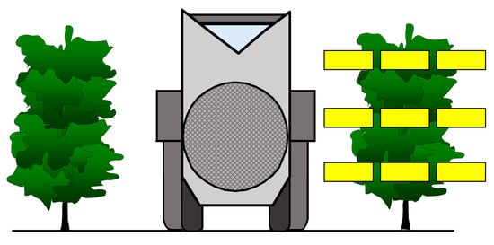
Figure 4.
Scheme of the water sensitive papers located in each vine for assessing the spraying coverage.
After each spray application, the WSP were collected, digitized using a scanner at a resolution of 600 dpi, 24 bits (color images), and processed with ImageJ® software (NIH, Bethesda, MD, USA), as established by Llop [37], in order to obtain the percentage of coverage.
2.8. Evaluation of the Biological Efficacy
Evaluation of the biological efficacy was carried out by comparing the presence of powdery mildew (Uncinula necator) in both the parcels treated with variable rate application (VRA), and in the parcels sprayed with conventional application (CONV). To achieve this process comparison, systematic sampling of 20 points ha−1 was implemented. Each sampling point (composed of three successive vines) was marked with a flag to maintain its location throughout the season. Two leaves were picked at random from each vine, and the percentage of infection was determined following the EPPO guideline [38].
In order to evaluate the efficacy, two different indexes were calculated for each studied parcel: (a) Incidence of powdery mildew (Equation (4)); and (b) degree of powdery mildew infestation (Equation (5)). The incidence refers to the number of leaves affected by powdery mildew independently of the severity of their infection.
The degree of infestation relates to the quantity of infested leaves and was classified based on the categories defined in Table 2.
Table 2.
Affectation categories based on the percentage of leaves affected, according to the EPPO guideline [34].
Two sampling processes were used throughout. The first sampling was arranged on July 5th (BBCH: Chardonnay 79; Merlot and Cabernet Sauvignon 77) and the second on July 31st (BBCH: Chardonnay 85; Merlot and Cabernet Sauvignon 83).
2.9. Statistical Analyses
For the evaluation of the water sensitive papers’ (WSP) coverage, one-way analysis of variance (ANOVA) was performed in order to evaluate the differences between vigor zones.
To evaluate the biological efficacy, the impact of the pesticide application type (conventional and variable rate application) was evaluated using one-way ANOVA for both incidence and infestation, considering vine variety as a covariate.
In all cases, previous to the analysis, the data were transforming using the arcsin function to obtain a normal distribution of residues. Statistical analyses were performed using SPSS 25.0 software [39].
3. Results and Discussion
3.1. Canopy Vigor Maps, Prescription Maps and Actual Variable Rate Application Maps
Three raw vigor maps were obtained throughout the duration of the season. These were obtained for each of the selected parcels from the spectral images taken from the multispectral camera that was mounted on the UAV. The raw vigor maps have a resolution of approximately 6 cm pxl−1 and allow for evaluation of the vegetation condition along the plot. This is the first step in determining the intra-plot variability. From this raw data, three classified canopy vigor maps were obtained for each plot during the growing season. Other previous works focused on using NDVI as an indicator for yield prediction and vineyard structural characteristics has also obtained satisfactory results distinguishing two or three different management zones according to NDVI [40,41,42].
Figure 5 indicates the 12 canopy vigor maps that were generated across the duration of the season. It was noted that these maps changed throughout the vineyard season. This result disagrees with the research of Kazmierski [43] that highlighted an intra-annual stability within vineyard season of NDVI patterns. However, this study used an airborne imaginary with a resolution of 3 m pxl−1 and only the last vineyard stages (85 days before harvest).
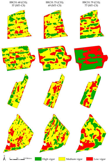
Figure 5.
Vigor maps for each parcel in the evaluated BBCH stages.
Table 3 presents the percentage of area corresponding to each vigor category for each generated canopy vigor map. It can be seen that the majority of the area corresponds to the medium vigor category, since this category includes quintiles 2, 3 and 4.
Table 3.
Percentage of area in each distinguished vigor map category (low—L, medium—M, high—H) in each parcel.
These results show the evolution of the intra-plot variability along the season, which was different for the three selected varieties. Cabernet Sauvignon (parcel 4) increased three times the percentage of high vigor zones, while in Merlot (plot 2) was multiplied by two. In all the varieties it was detected a decrease of surface corresponding to medium vigor zone. For the evaluation of these values shall be considered the influence of canopy management conducted during the period.
During the spraying season, a total of 28 spray applications were carried out (7 applications per plot studied). In each of these cases, the vegetation in each area of vigor was measured in order to determine the optimum volume of application using DOSAVIÑA® (Table 4) and thus create the prescription map. It is worth noting that canopy characterization follows the same tendency of vigor zones, finding the lowest high and width values in low vigor zones and the highest in the high vigor zones (Table 4) suggesting that NDVI has a good relationship with these two parameters. These results are consistence with those found in [16] where a significant relationship was obtained between LAI and NDVI (p < 0.001, R2 = 0.73) and [44] where was also describe a good correlation between LAI and NDVI (R2 = 0.92) and height and NDVI (R2 = 0.79).
Table 4.
Canopy characterization. Volume rate (L ha−1) calculated with Dosaviña® for each variety and canopy vigor (low, medium and high). Selected working conditions (color, number of nozzles and working pressure) for each pesticide application process (a for 1 to 4, b for 5 to 7).
Two of the prescription maps are shown as examples in Figure 6. The left side of the figure presents the prescription map built on June 20th, which corresponds to the 4th spray application of the season on parcel one. In this application, three different volumes of vegetation were determined. In red areas (low vigor), an optimum volume of 257 L ha−1 was determined. In the yellow areas (medium vigor) an optimum volume of 315 L ha−1 was determined, and in the blue areas (high vigor) an application volume of 372 L ha−1. Figure 6 right shows the prescription map built on July 12th, which corresponds to the 6th spray application of the season on parcel two. In this case, only two different vigor categories were differentiated. In green areas (low vigor), the volume rate was 230 L ha−1 and in the blue areas (high vigor), the volume rate was 370 L ha−1.
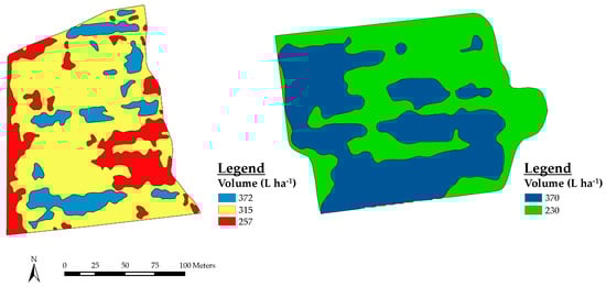
Figure 6.
Examples of prescription maps used in the field tests. Left: June 20th of parcel 1 (Chardonnay). Right: July 12th parcel 2 (Merlot).
In total, 28 actual application maps were downloaded from the touch screen of the prototype after the spray application processes. The actual application maps corresponding to the two examples previously referenced are presented in Figure 7. These maps present the real information about the application volume in these cases.
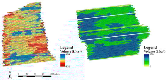
Figure 7.
Examples of actual application maps obtained in the field’s tests. Left: June 20th of parcel 1 (Chardonnay). Right: July 12th parcel 2 (Merlot).
3.2. Accuracy of the System
In order to quantify the correspondence between the prescription maps and the actual variable rate application maps, a range of eleven different thresholds were established, from 0% to 50% tolerance. The most restrictive threshold (0%) measured the percentage of points in which there was no difference between the intended and actual application rate. Conversely, the highest tolerance (50%) quantified the percentage of points where variations of ±50% of applied volume were detected.
In the case of the spray application on June 20th, previously presented as an example, only 1.3% of points were classified as successful points at the 0% threshold, while 99.8% of points were classified at the 50% threshold. Assuming a theoretical tolerance of ±10%, the system was able to classify 77.4% of the points as successful points. Figure 8 presents the distributed accuracy, classified according to the established threshold level. The red zones marked on the maps indicate the areas where the accuracy of the system exceeded the established thresholds. The majority of these red zones correspond to transition zones, these being zones where the sprayer was ordered to modify the working pressure. As can be seen by the results, the variable rate application method was capable of generate actual application maps with a good degree of accuracy when compared with prescription maps. Table 5 presents the percentage of points that were classified as successful points, assuming a ±10% tolerance across all parcels and spraying applications. Taking the average value of the data obtained, 77.0% of the points were classified as successful points. Similar results were obtained in other previous work [23] where a comparable variable rate system used in vineyard obtained an accuracy of 83% at ±10% tolerance. However, this last system was able to obtain a good accuracy (39%) at 0% tolerance. In case of field crops, where these types of systems are widely commercialized, Hørfarter [45] found a very good accuracy but using 1000 times less number of points for the comparison and calculating through a linear model between the intended and the actual application rate (R2 = 0.95).
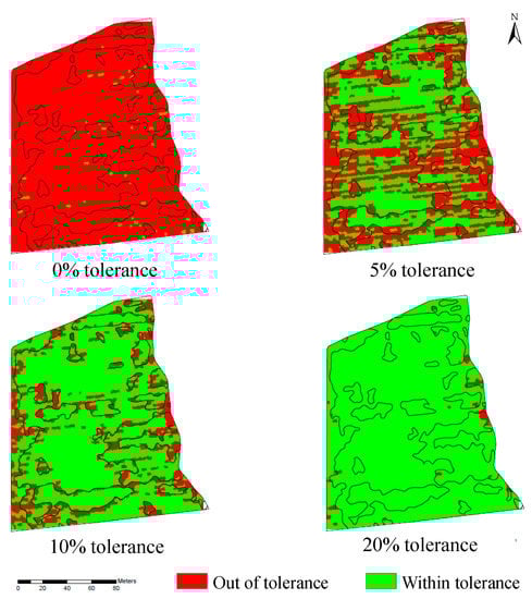
Figure 8.
Example of accuracy distribution classified according to 0, 5, 10 and 20% threshold.
Table 5.
Percentage of points classified as successful points, assuming a ±10% tolerance.
Observing the tendency in the accuracy values, it is clear that the precision of the system increases along the season. This fact can be observed for all the selected varieties. A potential explanation of this fact can be observed in Figure 5, where, in lines, it can be evaluated the changes of the distribution of the vigor zones on each parcel. A deep analysis of Figure 5 indicates high variability in the parcels at early stages. This fact generates more changes in the canopy vigor zones inside the parcel, which requires higher number of changes in the adjustment of working parameters of the sprayer. This fact reduces the accuracy value due to the fact that the pressure circuit in the sprayer requires certain time to re-adjust the pressure and stabilize the functioning. So, as larger is the number of transition points between zones of different canopy vigor, as reduced the accuracy of the system. These results are consistence with those found in [46,47] where was also determined that VRA technology operate more efficiently were the quantity of transitions zones decrease, due to the reduction of changes on working parameters in the sprayer (working pressure mainly).
3.3. Evaluation of Spray Distribution Quality
Coverage analysis, as displayed in Figure 9, indicates that promising results were obtained in all of the studied cases. Taking into account the average data, a coverage value of 35.1 ± 0.6% was observed. Despite changing the volume rate, no significant differences (p > 0.05) occurred in the coverage percentage across the vigor zones. In general, the coverage values seen during the spray applications ranged from 20 to 40%; it has been reported that this coverage is adequate to ensure pest/disease control in any spray application process [48]. These results support the case for adaptation of these applied volume rates to canopy characteristics, allowing for adjustment of the optimal amount of water while maintaining the coverage and spray distribution quality. Table 6 shows the detailed results obtained, both in terms of coverage (%) and of uniformity of distribution over the whole canopy, measured through the standard error of the mean (SEM). In general, the data did not indicate differences between the conventional and VRA systems, even if, in some cases, the volume rate was reduced according the canopy structure and dimensions. Similar results were obtained in other previous researches on variable application based on canopy characterization with on-board sensors [49,50,51].
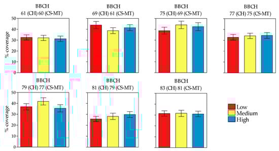
Figure 9.
Percentage of water sensitive papers coverage obtained each vigor. Mean of the parcels ± SEM.
Table 6.
Percentage of coverage (mean ± SE of the mean) for each vigor zone in each studied parcel.
Similar results were obtained at early crop stages with low canopy density, with high risk of overdosing. A deep analysis of coverage values (Table 6) indicates that the highest value of coverage (47.3%) was obtained for Chardonnay variety at medium canopy vigor level. In the opposite, the lowest value of coverage (27.8%) was obtained at Merlot variety, in this case at the low canopy density zones. Even if the statistical analysis demonstrated that grape variety had no influence in the obtained results, it is interesting to remark that, in terms of coverage, the highest average values of coverage were obtained at Chardonnay variety (42.9%), while the lowest were detected in Merlot variety (28.5%). Coverage values measured at the two plots of Cabernet Sauvignon were similar (34.3% for plot 3 and 34.2% for plot 4) and located between the other two varieties.
Figure 10 shows the improvement in coverage distribution in the whole canopy obtained when the applied volume was defined according the canopy structure (VRA) in comparison with the one obtained with the conventional spray application. It is clearly observed the improvements on spray uniformity.
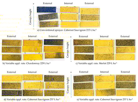
Figure 10.
Coverage (WSP) obtained with conventional spray application (CONV) (a), in comparison with coverage obtained at the four selected varieties when using variable rate application (VRA) (b–e).
3.4. Evaluation of the Biological Efficacy
Table 7 presents the results obtained for powdery mildew incidence and infestation in both types of pesticide application (conventional and variable rate application) within the two sampling periods. Generally, the incidences after the variable rate pesticide application parcels on July 5th were significantly lower than those obtained for the conventional spray process (8.4% vs. 23.1%, respectively). No significant differences were obtained, however, in the July 31st sampling (12.7% vs. 15.4%, respectively). In both cases, the statistical analysis shows that the covariate vine variety was not significant (p > 0.05). Regarding the degree of powdery mildew infestation, no significant differences were witnessed between the conventional and variable rate treatments (15.8% vs 19.3% on July 5th, and 16.5% vs. 17.2% on July 31st). In case of variable application rate based on prescription maps applied in field crops, which are mainly focused in weed control, have also proven to be effective [52].
Table 7.
Percentage of incidence and degree infestation of powdery mildew at two sampling dates for conventional (CONV) and variable rate application (VRA) parcels.
Figure 11 presents the applied volume rates for the conventional and variable rate application systems throughout the whole growing season. In the case of variable rate application, the volume rate was always related to the canopy characteristics. It followed the canopy development and other changes throughout the period, also accounting for vineyard management (pruning and stripping). In contrast, in conventional applications, the volume rate was largely invariable for all spray applications, with the exception being when the farmer detected any disease symptom. In these cases, the applied volume (and consequently the PPP dose) was doubled. This consequently risked losses to the soil, drift and led to difficulties with residue management. A specific example of this was with the Cabernet Sauvignon variety at BBCH 77, where the volume rate was upgraded from 200 to 400 L ha−1. Additionally, the arbitrary increase of volume application rate in conventional mode results in a very poor spray distribution, as it has been shown in Figure 10.
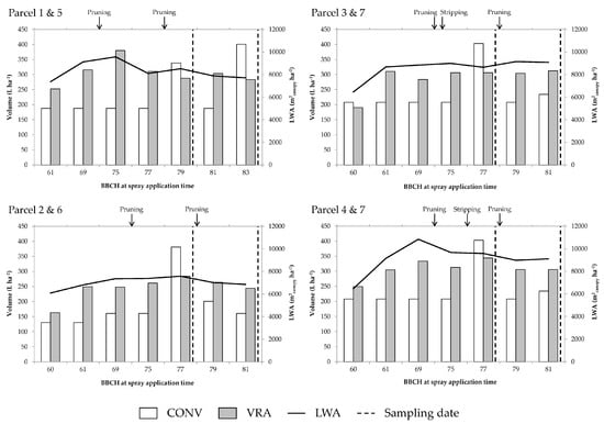
Figure 11.
Volume rate applied in conventional and variable rate parcels in each spray application. Time of the evaluation of the biological efficacy (sampling time) as well as pruning and stripping task are marked.
The biological efficacy results indicate that the incidence of powdery mildew at the first sampling date was significantly higher in the conventional parcels than in the variable rate application parcels. By using a volume rate that was not well adapted to the characteristics of the canopy, incidence of the disease increased, which, as described previously, forced the farmer to increase the volume rate application. Results corroborated the conclusions established by Balan [53] where demonstrated the great effect of spray application volume rate and working characteristics in the quality of the spray distribution and on risk of contamination.
4. Conclusions
In this study, a prototype variable rate application system, based on prescription maps, was tested throughout the duration of an entire vineyard growth season. The major findings were found to be:
- The classified vigor maps were simply transformed into prescription maps by taking into account the structural canopy characteristics;
- The system was able to read a prescription map and appropriately modify the working parameters (working pressure) depending on the position of the sprayer in the field;
- A system accuracy of approximately 80% was obtained, assuming a tolerance of 10% deviation;
- Despite changing the working pressure and volume rate between the vigor zones, the coverage values that were obtained during the spray applications can be considered similar in all cases. The coverage was also deemed adequate in minimum terms to ensure pest/disease control in all cases;
- The variable rate application process, based on the combination of vigor maps with the DSS Dosaviña® to determine the optimal volume rate, can obtain equivalent results regarding biological efficacy as a conventional pest application process;
The variable rate application process allows an improved and more reasonable use of PPP, by taking into considering the specific characteristics of the intended target (canopy), when compared with a conventional spraying process. This results in a safer, and more sustainable, use of pesticides throughout the entire growing season.
Author Contributions
Methodology, J.C., M.G., J.L., R.S. and E.G.; investigation, J.C., M.G., J.L., P.O., R.S. and E.G.; data curation, J.C. and M.G.; writing—original draft preparation, J.C., M.G. and E.G.; writing—review and editing, E.G.; project administration, E.G. and J.C. All authors have read and agreed to the published version of the manuscript.
Funding
This research was developed with partial funding from the FI-AGAUR grant from the Generalitat de Catalunya (2017 FI_B 00893).
Acknowledgments
The authors would like to thank to Miguel Torres and Jean Leon for their support in the field trials and Estel Grup S.L. for providing the electronic controller WAATIC and for the technical monitoring of the system during the whole season.
Conflicts of Interest
The authors declare no conflict of interest.
References
- Giles, D.; Billing, R. Deployment and performance of a uav for crop spraying. Chem. Eng. Trans. 2015, 44, 307–312. [Google Scholar] [CrossRef]
- Miranda-Fuentes, A.; Llorens, J.; Rodriguez-Lizana, A.; Cuenca, A.; Gil, E.; Blanco-Roldán, G.L.; Gil-Ribes, J. Assessing the optimal liquid volume to be sprayed on isolated olive trees according to their canopy volumes. Sci. Total Environ. 2016, 568, 269–305. [Google Scholar] [CrossRef]
- Gil, E.; Campos, J.; Ortega, P.; Llop, J.; Gras, A.; Armengol, E.; Salcedo, R.; Gallart, M. Dosaviña: Tool to calculate the optimal volume rate and pesticide amount in vineyard spray applications based on a modified leaf wall area method. Comput. Electron. Agric. 2019, 160, 117–130. [Google Scholar] [CrossRef]
- Siegfried, W.; Viret, O.; Huber, B.; Wohlhauser, R. Dosage of plant protection products adapted to leaf area index in viticulture. Crop Prot. 2007, 26, 73–82. [Google Scholar] [CrossRef]
- Furness, G.O.; Thompson, A.J. Using point of first run-off and spray volume in litres per 100 metres per metre of canopy height for setting pesticide dose. Agric. Eng. Int. Gigr. Ejournal 2008, 10, 08006. [Google Scholar]
- Walklate, P.J.; Cross, J.V.; Pergher, G. Support system for efficient dosage of orchard and vineyard spraying products. Comput. Electron. Agric. 2011, 75, 355–362. [Google Scholar] [CrossRef]
- Chen, Y.; Zhu, H.; Ozkan, H.E. Development of a variable-rate-sprayer with laser scanning sensor to synchronize sprayer outputs to tree structures. Trans. ASABE 2012, 55, 773–781. [Google Scholar] [CrossRef]
- Codis, S.; Douzals, J.P. Comparaison des systèmes d’expression des doses de produits de protection de la vigne dans 5 pays européens et les besoins d’une harmonisation. In Proceedings of the AFPP-CIETAP-Conference Sur Les Techniques D’application de Produits de Protection des Plantes, Lyon, France, 15–16 March 2012; p. 10. [Google Scholar]
- Gil, E.; Gallart, M.; Llorens, J.; Llop, J.; Bayer, T.; Carvalho, C. Spray adjustments based on LWA concept in vineyard. Relationship between canopy and coverage for different application settings. In Proceedings of the Aspects of Applied Biology 122, International Advances in Pesticide Application, Oxford, UK, 8–10 January 2014; pp. 25–32. [Google Scholar]
- Garcerá, C.; Fonte, A.; Moltó, E.; Chueca, P. Sustainable use of pesticide applications in citrus: A support tool for volume rate adjustment. Int. J. Environ. Res. Public Health 2017, 14, 715–728. [Google Scholar] [CrossRef] [PubMed]
- Du, Q.; Chang, N.B.; Yang, C.; Srilakshmi, K.R. Combination of multispectral remote sensing, variable rate technology and environmental modeling for citrus pest management. J. Environ. Manag. 2008, 86, 14–26. [Google Scholar] [CrossRef]
- Escolà, A.; Rosell-Polo, J.R.; Planas, S.; Gil, E.; Pomar, J.; Camp, F.; Llorens, J.; Solanelles, F. Variable rate sprayer Part 1—Orchard prototype: Design, implementation and validation. Comput. Electron. Agric. 2013, 95, 122–135. [Google Scholar] [CrossRef]
- Gil, E.; Llorens, J.; Llop, J.; Escolà, A.; Rosell-Polo, J.R. Variable rate sprayer. Part 2—Vineyard 1 prototype: Design, implementation and validation. Comput. Electron. Agric. 2013, 95, 136–150. [Google Scholar] [CrossRef]
- De Castro, A.I.; Jiménez-Brenes, F.M.; Torres-Sánchez, J.; Peña, J.M.; Borra-Serrano, I.; López-Granados, F. 3-D characterization of vineyards using a novel UAV imagery-based OBIA procedure for precision viticulture applications. Remote Sens. 2018, 10, 584. [Google Scholar] [CrossRef]
- Hall, A.; Lamb, D.W.; Holzapfel, B.; Louis, J. Optical remote sensing applications in viticulture – A review. Aust. J. Grape Wine Res. 2002, 8, 36–47. [Google Scholar] [CrossRef]
- Johnson, L.F.; Roczen, D.E.; Youkhana, S.K.; Nemani, R.R.; Bosch, D.F. Mapping Vineyard leaf area with multispectral satellite imagery. Comput. Electron. Agric. 2003, 38, 37–48. [Google Scholar] [CrossRef]
- Baluja, J.; Diago, M.P.; Balda, P.; Zorer, R.; Meggio, F.; Morales, F.; Tardaguila, J. Assessment of vineyard water status variability by thermal and multispectral imagery using an Unmanned Aerial Vehicle (UAV). Irrig. Sci. 2012, 30, 511–522. [Google Scholar] [CrossRef]
- Albetis, J.; Duthoit, S.; Guttler, F.; Jacquin, A.; Goulard, M.; Poilvé, H.; Féret, J.-B.; Dedieu, G. Detection of Flavescence dorée grapevine disease using Unmanned Aerial Vehicle (UAV) multispectral imagery. Remote Sens. 2017, 9, 308. [Google Scholar] [CrossRef]
- Mathews, A.J.; Jensen, J.L.R. Visualizing and quantifying vineyard canopy LAI using an Unmanned Aerial Vehicle (UAV) collected high density structure from motion point cloud. Remote Sens. 2013, 5, 2164–2183. [Google Scholar] [CrossRef]
- Ballesteros, R.; Ortega, J.F.; Hernández, D.; Moreno, M.Á. Characterization of Vitis vinifera L. canopy using unmanned aerial vehicle-based remote sensing and photogrammetry techniques. Am. J. Enol. Vitic. 2015, 66, 120–129. [Google Scholar] [CrossRef]
- Poblete-Echeverría, C.; Olmedo, G.F.; Ingram, B.; Bardeen, M. Detection and segmentation of vine canopy in ultra-high spatial resolution rgb imagery obtained from Unmanned Aerial Vehicle (UAV): A case study in a commercial vineyard. Remote Sens. 2017, 9, 268. [Google Scholar] [CrossRef]
- Weiss, M.; Baret, F. Using 3D point clouds derived from UAV RGB imagery to describe vineyard 3D macro-structure. Remote Sens. 2017, 9, 111. [Google Scholar] [CrossRef]
- Campos, J.; Llop, J.; Gallart, M.; García-Ruíz, F.; Gras, A.; Salcedo, R.; Gil, E. Development of canopy vigor maps using UAV for site-specific management during vineyard spraying process. Precis. Agric. 2019, 20, 1136–1156. [Google Scholar] [CrossRef]
- EU. Directive 2009/128/EC of the European Parliament and of the Council of 21 October 2009 Establishing a Framework for Community Action to Achieve the Sustainable Use of Pesticides. Off. J. Eur. Union 2009, 309, 71–86. [Google Scholar]
- Vogel, J.W.; Wolf, R.E.; Dille, A. Evaluation of a Variable Rate Application System for Site-Specific Weed Management. In Proceedings of the 2005 ASAE Annual Meeting (p. 1); American Society of Agricultural and Biological Engineers: St. Joseph, MI, USA, 2005; Paper No. 051120. [Google Scholar]
- Michaud, M.; Watts, K.C.; Percival, D.C.; Wilkie, K.I. Precision pesticide delivery based on aerial spectral imaging. Can. J. Biosyst. Eng. 2008, 50, 2.9–2.15. [Google Scholar]
- D’Amico, M.; Coppola, A.; Chinnici, G.; Di Vita, G.; Pappalardo, G. Agricultural systems in the European Union: An analysis of regional differences. New Medit. 2013, 12, 28–34. [Google Scholar]
- European Commission. Precision Agriculture: An Opportunity for EU Farmers—Potential Support with the CAP 2014–2020; European Commission Agriculture and Rural Development: Brussels, Belgium, 2014. [Google Scholar]
- European Commission. Structure and Dynamics of EU Farms: Changes, Trends and Policy Relevance. In EU Agricultural Economics Briefs, 9; European Commission Agriculture and Rural Development: Brussels, Belgium, 2013. [Google Scholar]
- Meier, U. BBCH-Monograph. In Growth Stages of Plants-Entwicklungsstadien von Planzen—Estadios de Las Plantas-Développement des Plantes; Blackwell Wissenschaftsverlag: Berlin, Germany; Wien, Austria, 1977; p. 622. [Google Scholar]
- Rouse, J.W.; Haas, R.H.; Schell, J.A.; Deering, D.W. Monitoring vegetation systems in the Great Plains with ERTS. In Proceedings of the Third ERTS Symposium, NASA SP-351, Washington, DC, USA, 10–14 December 1973; pp. 309–317. [Google Scholar]
- QGIS Development Team. QGIS Geographic Information System. Open Source Geospatial Foundation. Available online: http://qgis.osgeo.org (accessed on 12 May 2018).
- EPPO. Standard Measurement Procedure in High Growing Crop Trials. Available online: https://www.eppo.int/media/uploaded_images/ACTIVITIES/plant_protect_products/Dose_exp_measure_procedure.pdf (accessed on 20 May 2018).
- Bartier, P.M.; Keller, C.P. Multivariate interpolation to incorporate thematic surface data using inverse distance weighting (IDW). Comput. Geosci. 1996, 22, 795–799. [Google Scholar] [CrossRef]
- Gil, E.; Escolà, A. Design of a decision support method to determine volume rate for vineyard spraying. Appl. Eng. Agric. 2009, 25, 145–151. [Google Scholar] [CrossRef]
- Miranda-Fuentes, A.; Rodríguez-Lizana, A.; Gil, E.; Agüera-Vega, J.; Gil-Ribes, J. Influence of liquid-volume and air flow rates on spray application quality and homogeneity in super-intensive olive tree canopies. Sci. Total Environ. 2015, 537, 250–259. [Google Scholar] [CrossRef]
- Llop, J.; Gil, E.; Gallart, M.; Contador, F.; Ercilla, M. Spray distribution evaluation of different setting of a hand-held trolley sprayer used in green house tomato crops. Pest Manag. 2015, 72, 505–516. [Google Scholar] [CrossRef]
- OEPP/EPPO. Guidelines for the Biological Evaluation of Fungicides: Plasmopara viticola. Bulletin OEPP/EPPO 2002, 31, 315–318. [Google Scholar]
- IBM Corp. IBM SPSS Statistics for Windows, Version 25.0; IBM Corp: Armonk, NY, USA, 2017. [Google Scholar]
- Acevedo-Opazo, C.; Tisseyre, B.; Guillaume, S.; Ojeda, H. The potential of high spatial resolution information to define within-vineyard zones related to vine water status. Precis. Agric. 2008, 9, 285–302. [Google Scholar] [CrossRef]
- Martinez-Casasnovas, J.; Agelet-Fernandez, J.; Arno, J.; Ramos, M. Analysis of vineyard differential management zones and relation to vine development, grape maturity and quality. Span. J. Agric. Res. 2012, 10, 326–337. [Google Scholar] [CrossRef]
- Bonilla, I.; Martínez de Toda, F.; Martínez-Casasnovas, J.A. Vine vigor, yield and grape quality assessment by airborne remote sensing over three years: Analysis of unexpected relationships in cv. Tempranillo. Span. J. Agric. Res. 2015, 13. [Google Scholar] [CrossRef]
- Kazmierski, M.; Glemas, P.; Rousseau, J.; Tisseyre, B. Temporal stability of within-field patterns of NDVI in non-irrigated Mediterranean vineyards. J. Int. Sci. Vigne Vin 2011, 45, 61–73. [Google Scholar] [CrossRef]
- Montero, F.J.; Meliá, J.; Brasa, A.; Segarra, D.; Cuesta, A.; Lanjeri, S. Assessment of vine development according to available water resources by using remote sensing in La Mancha, Spain. Agric. Water Manag. 1999, 40, 363–375. [Google Scholar] [CrossRef]
- Hørfarter, R.; Thorsted, M.D.; Stougård, K.; Poulsen, H.V. Precision spraying by combining a variable rate application map with an on/off map. Precision agriculture ’19. In Proceedings of the 12th European Conference on Precision Agriculture, Montpellier, France, 8–11 July 2019; pp. 53–59. [Google Scholar] [CrossRef]
- Zhang, N.; Wang, M.; Wang, N. Precision agriculture—A worldwide overview. Comput. Electron. Agric. 2002, 6, 113–132. [Google Scholar] [CrossRef]
- Arnó, J.; Martínez-Casasnovas, J.A.; Ribes-Dasi, M.; Rosell, J.R. Review. Precision Viticulture. Research topics, challenges and opportunities in site-specific vineyard management. Span. J. Agric. Res 2009, 7, 779–790. [Google Scholar]
- Chen, Y.; Ozkan, H.E.; Zhu, H.; Derk sen, R.C.; Krause, C.R. Spray de position in side tree canopies from a newly developed variable-rate air-assisted sprayer. Trans. ASABE 2013, 56, 1263–1272. [Google Scholar]
- Solanelles, F.; Escolà, A.; Planas, S.; Rosell, J.; Camp, F.; Gràcia, F. An electronic control system for pesticide application proportional to the canopy width of tree crops. Biosyst. Eng. 2006, 95, 473–481. [Google Scholar] [CrossRef]
- Gil, E.; Escolà, A.; Rosell, J.; Planas, S.; Val, L. Variable rate application of plant protection products in vineyard using ultrasonic sensors. Crop Prot. 2007, 26, 1287–1297. [Google Scholar] [CrossRef]
- Balsari, P.; Doruchowski, G.; Marucco, P.; Tamagnone, M.; Van De Zande, J.; Wenneker, M. A system for adjusting the spray application to the target characteristics. Agric. Eng. Int. CIGR J. 2008, 10, 1–11. [Google Scholar]
- Carrara, M.; Comparetti, A.; Febo, P.; Orlando, S. Spatially variable rate herbicide application on Durum wheat in Sicily. Biosyst. Eng. 2004, 87, 387–392. [Google Scholar] [CrossRef]
- Balan, M.G.; Saab, O.J.G.A.; Ecker, A.E.A.; Migliorini, G.O. Description of the Application Method in Technical and Scientific Work on Insecticides. Acta Sci. Agron. 2016, 38, 9–17. [Google Scholar] [CrossRef][Green Version]
© 2020 by the authors. Licensee MDPI, Basel, Switzerland. This article is an open access article distributed under the terms and conditions of the Creative Commons Attribution (CC BY) license (http://creativecommons.org/licenses/by/4.0/).