Deep Learning for Mango (Mangifera indica) Panicle Stage Classification

Abstract

Automated assessment of the number of panicles by developmental stage can provide information on the time spread of flowering and thus inform farm management. A pixel-based segmentation method for the estimation of flowering level from tree images was confounded by the developmental stage. Therefore, the use of a single and a two-stage deep learning framework (YOLO and R²CNN) was considered, using either upright or rotated bounding boxes. For a validation image set and for a total panicle count, the models MangoYOLO(-upright), MangoYOLO-rotated, YOLOv3-rotated, R²CNN(-rotated) and R²CNN-upright achieved weighted F1 scores of 76.5, 76.1, 74.9, 74.0 and 82.0, respectively. For a test set of the images of another cultivar and using a different camera, the R² for machine vision to human count of panicles per tree was 0.86, 0.80, 0.83, 0.81 and 0.76 for the same models, respectively. Thus, there was no consistent benefit from the use of rotated over the use of upright bounding boxes. The YOLOv3-rotated model was superior in terms of total panicle count, and the R²CNN-upright model was more accurate for panicle stage classification. To demonstrate practical application, panicle counts were made weekly for an orchard of 994 trees, with a peak detection routine applied to document multiple flowering events.

1. Introduction

Mango (Mangifera indica) trees produce panicles bearing hundreds of inconspicuous flowers, of which at most three or four flowers will develop fruit, although frequently only one or none will so develop. The assessment of the number of panicles on a tree thus sets a maximum potential for the crop yield of that season, while the assessment of the stage of panicle development is useful for assessment of the time spread of flowering, and thus the likely time spread of the harvest period. Mapping areas of early flowering can also guide selective early harvesting and panicle detection can inform selective spraying operations. However, the manual assessment and recording of panicle number and stage is a tedious task that relies on the experience of the observer. An automated approach for detection and classification of flowering stage could thus aid orchard management.

Machine vision has been applied for the assessment of the level of flowering for several tree crops where the flowers are easily distinguishable from the background based on colour thresholding. For example, [1] reported a prediction accuracy of 82% on apple flower count, relative to a manual count, [2] achieved a coefficient of determination (R²) of 0.94 between machine vision and manual count of tangerine flowers, [3] claimed an average detection rate of 84.3% on peach flowers, [4] reported a R² of 0.59 between machine vision and manual count of apple flower cluster counts, [5] obtained a F1-score of 73% for tomato flower detection, and [6] avoided a direct count of flowers, but rather characterised almond ‘flowering intensity’ in terms of a ratio of flower and canopy pixels, reporting a poor relationship (R² = 0.23) for this index for a given tree between two seasons. However, all these reports were based on segmentation routines, generally involving colour given the obvious colour difference for flowers of these species and background. This approach is expected to perform poorly for tree crops for which the colour difference between vegetative and reproductive tissue is not marked.

Furthermore, apple, peach and tomato flowers are relatively conspicuous. A mango tree produces panicles with pale cream flowers a few mm in size. The panicle size changes with developmental stage, increasing through the stages of bud break, ‘asparagus’, elongation, anthesis (flower opening) to the full bloom ‘Christmas tree’ stage, then decreasing with flower drop. Panicle structure is thus more complex than that of a single flower. Therefore, machine vision detection of mango panicles is more challenging compared to the detection of the single flowers of apple, citrus and almond trees.

There are few reports on use of machine vision for the assessment of the number of flowering panicles involving a branched inflorescence with many inconspicuous flowers. For example, [7] used intensity level in CIE LAB colour space in assessment of the number of grape flowers in inflorescences imaged against a black background. A R² of 0.84 against human count was achieved. In [8], researchers used Scale-invariant Feature Transform (SIFT) descriptors/features along with a Support Vector Machine (SVM) to detect rice flower panicles in images, with a R² of 0.67 against a human count achieved.

Recent review papers have emphasised the use of neural network and deep learning in agricultural machine vision in general [9] and for fruit detection and yield estimation [10]. For example, [11] noted that better performance in fruit detection and localization was achieved through the use of neural networks compared to traditional models based on colour thresholding and hand-engineered feature extraction methods. The use of lighter weight, single shot detectors which allow faster computation times is introduced in [12]. Our group designed a modified You Only Look Once (YOLO, [13]) architecture, ‘MangoYOLO’ [12] which was demonstrated to be superior to YOLOv3 [14] for the application of fruit detection and count. In [15], researchers used Clarifai [16] Convolutional Neural Network (CNN) architecture to extract features from the possible flower regions obtained from super-pixel segmentation followed by SVM [17] for flower detection. For apple, peach and pear datasets, this method outperformed other methods of that time that were based on SVMs and Hue-Saturation-Value (HSV) colour thresholding methods. Extending their earlier work, [18] used a Fully Convolutional Neural Network (FCN) from [19] for flower detection on tree images of apple, peach and pear. A region growing refinement (RGR) algorithm was implemented to refine the segmentation output from FCN. This method achieved F1 scores of 83.3%, 77.3%, 74.2% and 86% on two apple, peach and pear flower datasets respectively, outperforming their previous Clarifai CNN method [15] and the HSV colour model. Deep learning methods of object detection may suit the task of detection and counting of mango panicles by developmental stage, through automatic learning of useful features for classification [10].

Our group has previously considered the use of machine vision to assess mango flowering. In [20,21], researchers used the traditional method of pixelwise segmentation to segment panicle pixels from canopy pixels, with results expressed either as panicle pixel count per tree or as the ratio of panicle to canopy pixel count (termed ‘flowering intensity’). This procedure was implemented on images obtained at night using artificial lighting, processed with a colour threshold followed by SVM classification to refine the segmentation results. The use of a Faster R-CNN [22] deep learning technique to count panicles was reported by [21]. This work was limited to estimation of the extent of flowering and the time of peak flowering event. A R² of 0.69 between machine-vision flowering intensity and in-field human count of panicles per tree for 24 trees was reported for the segmentation method, while a R² of 0.78 and 0.84 was reported for deep learning Faster R-CNN framework with dual and multi-view imaging approaches, respectively.

These earlier reports employed upright bounding boxes. The use of an annotation bounding box as tight as possible around the objects has been recommended to avoid background noise in the training image sets [10]. However, panicles are oriented in some range of angles. Upright bounding boxes will therefore not fit tightly around the object perimeter (Figure 1), and a larger amount of background signal will be included in the object class for training. This could adversely affect the classification accuracy of the model.

There are several methods that involve use of rotated bounding boxes. The two-stage detector R²CNN (Rotational Region CNN for Orientation Robust Scene Text Detection) [23] is a modification of the Faster R-CNN object detection framework used to incorporate training on rotated bounding box annotations for detecting arbitrarily-oriented objects in images. This modified framework seems suited to the task of panicle detection. Alternatively, the single stage detector YOLO allows a number of data augmentation measures, including the random rotation of the labelled bounding boxes during training by a range (degrees) specified by the user in the configuration file.

In the current paper, the task of panicle detection task and count is extended to another level through classification to developmental stage, with comparison of a large (R²CNN framework with ResNet101 CNN) and a small (YOLO framework with MangoYOLO CNN) object detection architecture, and consideration of the use of rotated, compared to upright, bounding boxes. To the authors’ knowledge, the current study is the first to classify the stage of flowering for an on-tree fruit crop and is the first report on use of the rotated bounding box method of R²CNN for flower panicle detection. The current study utilized the imaging hardware used by [21], allowing for a direct comparison of results of the traditional machine learning approach used by [21]. Field relevance was demonstrated by assessment of orchard flowering at regular intervals (e.g., weekly) to provide information on timing of flowering peaks, for use in estimation of harvest timing. The major contributions of this study are thus (i) the comparison of single and double-staged deep learning object detection frameworks for flowering panicle detection and development stage classification; (ii) the comparison of deep learning methods with traditional segmentation method; (iii) the comparison of model performance with respect to the use of rotated and upright bounding box annotations; (iv) the application of a peak-detection routine to assist in the identification of a flowering event in a time series; (v) an approach to assess/visualize flowering data to inform farm management.

2. Materials and Methods

2.1. Image Acquisition

Tree images of orchard A (

Table 1. Orchard and imaging description.

Orchard Name	Location (lat., long.)	Cultivar	Camera	Image Resolution
Orchard A	−23.032749, 150.620470	Honey Gold	Basler	2464 × 2048 pixels
Orchard B	−25.144, 152.377	Calypso	Canon	6000 × 4000 pixels

) were acquired at night every week from 16 August to 18 October 2018, using a 5 MP Basler acA2440-75 µm RGB camera and a lighting rig (700 W LED floodlight) mounted on a farm vehicle driven at a speed of about 5 km/h, with triggering of the camera at every tree position from a GNSS device, and the display of data on a web-app farm map as described by [21]. The orchard contained 994 trees, and thus each weekly imaging event captured 1,988 images. This time window covered the flowering period of this orchard, from panicle formation to fruit set.

The image set of 24 trees from orchard B (Table 1; from [21]) were used as a test set. In that study, images were acquired using a 24 MP Canon (DSLR 750D) camera. The number of open, flowering panicles on these trees was manually counted. For both orchards, trees were imaged from each side, with a view from each inter-row (‘dual-view’ imaging).

2.2. Data Preparation

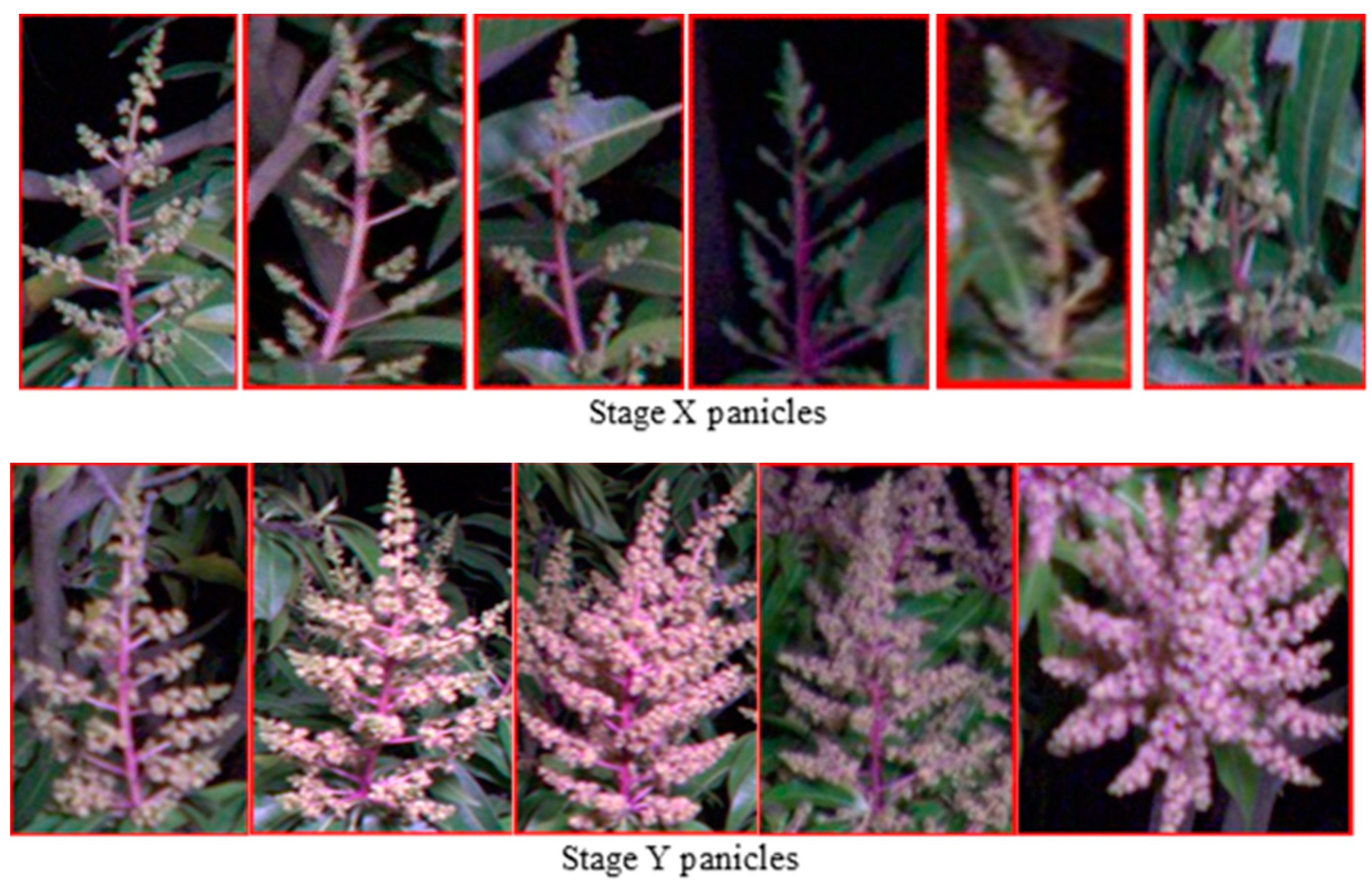
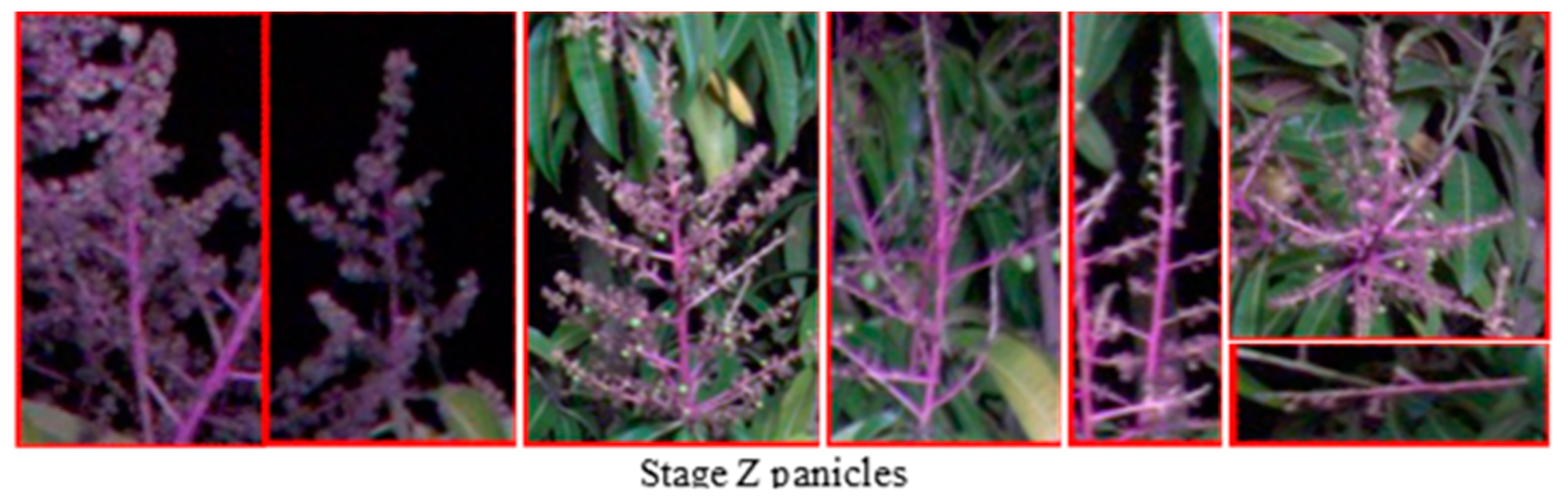
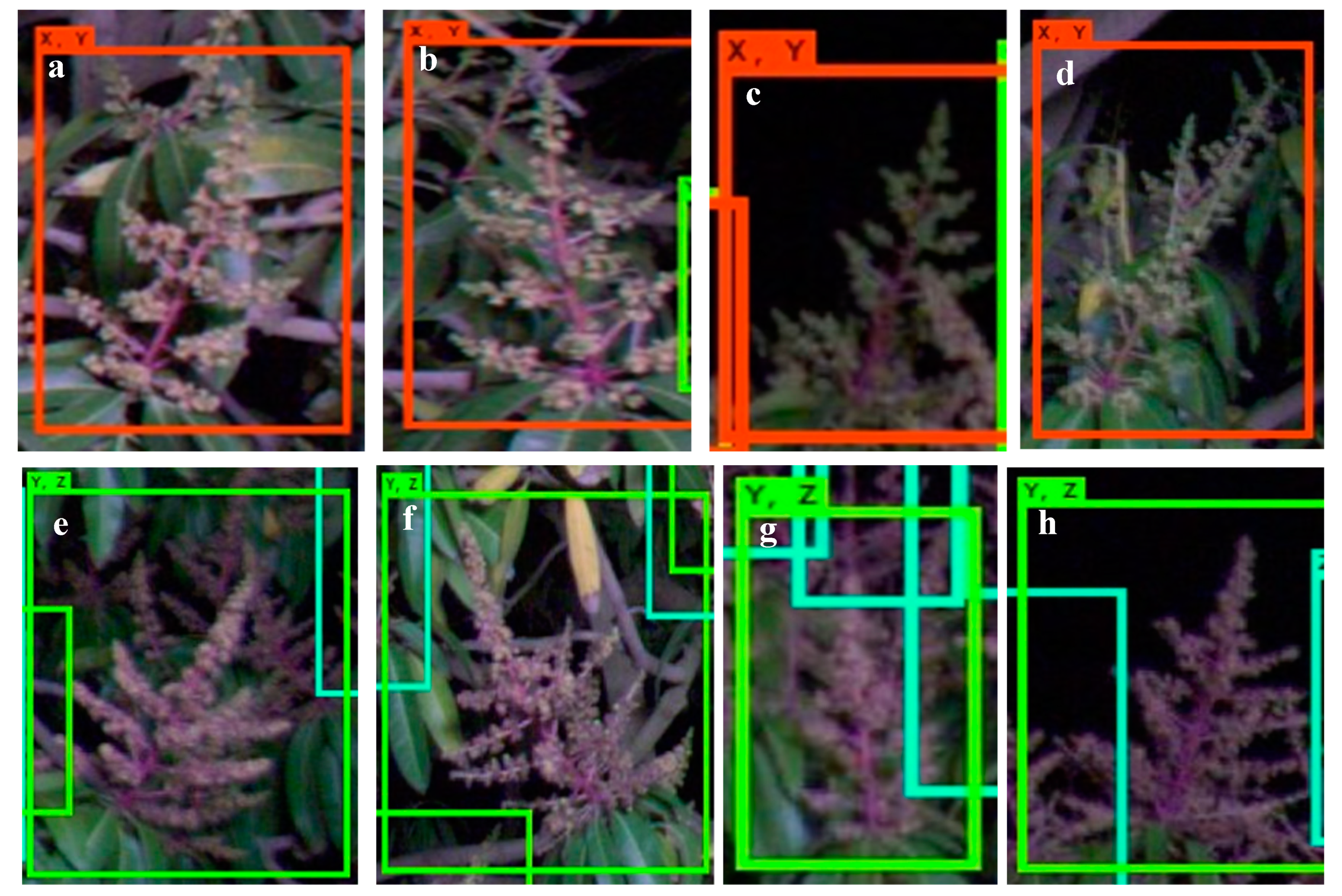
2.2.1. Image Annotation and Labelling

Mango panicles in the training image sets were categorized into three stages; (i) stage X—panicles with flowers (whitish in colour) that were not fully opened, i.e., flower opening to inflorescence branching (Figure 2, top row); (ii) stage Y—panicles with open flowers, colloquially known as ‘Christmas tree’ stage (Figure 2, middle row); (iii) stage Z—panicles displaying flower drop and fruit set (Figure 2, bottom row). A four-category system was initially trialled, but human differentiation of the two early stages was problematic, and the resulting model performance was poorer than for the three-category system (data not shown).

Annotation was done using roLabelImg (https://github.com/cgvict/roLabelImg) which is a modification of LabelImg (a graphical image annotation tool) to incorporate rotated boxes. Images were opened in roLabelImg software and a rectangular bounding box was drawn and rotated by dragging to fit nicely around each panicle. Each box was labelled with their respective class name (X or Y or Z). For each image, annotations were saved as XML files which contained the label (class name or category) and the position (height, width and centre co-ordinates of the box) of each annotated box along with the orientation angle.

As the annotations prepared for training R²CNN contained rotated bounding boxes which cannot be used directly with the YOLO model, a separate python script was written to convert the rotated bounding box annotations to upright bounding box annotations for training of the YOLO model. The boundingRect function from open source computer vision library (OpenCV) [24] was utilized to obtain an upright bounding box from the vertices of a rotated bounding box as contour input to the function. A visualization of the rotated ground truth boxes and the transformed upright bounding box annotation is presented in Figure 3. Separate Python scripts were written to convert the XML annotation format of roLabelImg to that of R²CNN and YOLO formats for model training.

2.2.2. Training, Validation and Test Sets

Training was based on 54 images (3178 labelled panicles) of trees from orchard A (

Table 2. Of panicles in training, validation and test image sets. The test set consisted of manual panicle counts per tree from [21] and Canon camera images of those trees (no panicle stage categorization was available).

	Number of Images	Number of Panicles			Total
		Stage X	Stage Y	Stage Z
Training set	54	1007	1107	1064	3178
Validation set	6	167	316	122	635
Test set	48	-	-	-	2853

), with images drawn from different weeks. A validation set was assembled from images of one side of a single orchard A tree, acquired over a six-week period (Table 2). These images were not included in the training set.

The training dataset also included annotations for background (369 snips), as required for R²CNN training. R²CNN uses the background class for negative hard-data mining and was not treated as a detection class during inference. However, the YOLO object detection framework does not require a background class, as all parts of the images other than those having bounding box for training are automatically treated as background. Therefore, the background class was not used for YOLO model performance evaluation.

The test set (Table 2) was an independent set consisting of images of orchard B, from the study of [21]. These images were of trees of a different cultivar and from a different orchard, and acquired with a different camera, to that of the training and validation sets.

2.2.3. Computing

Model training and testing was implemented on the CQUniversity High Performance Computing (HPC) facility graphics node with following specifications: Intel^® (Santa Clara, California, U.S.A.) Xeon^® Gold 6126 (12 cores, 2600MHz base clock) CPU, NVIDIA^® (Santa Clara, California, U.S.A.) Tesla^® (San Carlos, California, U.S.A) P100 (16 GB Memory, 1328 MHz base clock, 3584 CUDA cores) GPU. Red Hat (Raleigh, North Carolina, U.S.A.) Enterprise Linux Server 7.4 (Maipo) and 384GB RAM. CUDA v9.0, cuDNN v7.1.1, OpenCV v3.4.0, Python v2.7.14, GCC v4.8.5, scikit-learn v0.19.1, tensorflow-gpu v1.6.0, Keras v2.1.5, Cython v0.28.

Images (of two sides) of each tree were fed to the model for detection and classification. For each image of a tree, the results (number of each stage panicles) were saved as a text file and later uploaded along with the GNSS position to the ‘fruitMaps’ website for display on a farm map as described in [21].

2.3. Detection and Classification Models

The pixel segmentation method used in [21] was employed using the settings of [20]. Mango panicle classification at three developmental stages was attempted using the following architectures:

YOLOv3-rotated: The single shot object detection framework YOLOv3 [14] is deeper but more accurate than its previous versions [13,25]. The configuration file data augmentation feature to allow rotation of images during training was enabled for this training exercise. Images were rotated randomly in the range of 40 degrees to mimic the natural range of panicle orientations in tree images. Network input resolution was set to 1024 × 1024 pixels following the YOLO requirement that the input images are square, and resolution is a multiple of 32. This resolution can be changed to higher values but at the cost of higher computation memory and slower train/test speed. Four classes (3 stages and 1 background class) were used in training, however the detection of the background class was ignored during model performance evaluation. The model was trained for 35.7 k iterations with a batch size of 32 and data augmentation techniques defaulted to the YOLOv3 settings (saturation = 1.5, exposure = 1.5, hue = 0.1). The learning rate and momentum were set to the default values of 0.001 and 0.9 respectively. No transfer learning was employed, with the weights of the convolution neural network initialized at random values. Finally, saved model weights from 33 k iteration was used for testing and validation.

MangoYOLO-rotated: MangoYOLO was originally conceived for on-tree mango fruit detection, and has an architecture based on the YOLOv3 [14] object detection framework, optimized for better speed and accuracy. In this architecture, a YOLO deep learning object detection framework is used with a MangoYOLO CNN classifier [12]. The training parameters for YOLOv3-rotated were retained for MangoYOLO-rotated model training. Images were rotated randomly in the range of 40 degrees. The model was trained for 77.5 k iterations with a batch size of 32. Finally, the saved model weights from 77.4 k iteration were used for testing and validation.

MangoYOLO(-upright): MangoYOLO(-upright) is same as MangoYOLO-rotated except the random image rotation feature in the MangoYOLO-rotated configuration file was turned off, as was the case in the fruit detection work of [12]. The model was trained for 89.5 k iterations with a batch size of 32. Finally, saved model weights from the 66 k iteration were used for testing and validation.

R²CNN(-rotated): R²CNN(-rotated) is basically a Faster R-CNN object detection framework with a modification to support training on rotated objects. The R²CNN(-rotated) implementation supported only three CNN architectures - mobilenet_v2, ResNet50_v1 and resnet101_v1. Given that deeper CNN models generally produce better results in terms of object detection and classification, ResNet101_v1 CNN architecture was used with R²CNN(-rotated) framework for model training. The tensorflow re-implementation of R²CNN (https://github.com/DetectionTeamUCAS/R2CNN_Faster-RCNN_Tensorflow) was used for training and testing in this study. All model training parameters were set to the default values. With R²CNN(-rotated), as for Faster R-CNN, the input resolution can be set to be square or the original aspect ratio can be preserved (shorter side scaled to 800 pixels and longer side scaled accordingly). The original Basler images 2464 × 2048 pixels automatically resized to 962 × 800 pixels during training and testing. The RGB channel pixel mean values were initialized with the values (R = 41.647, G = 41.675, B = 43.048) calculated of the training dataset. The model was trained for 146 k iterations with a batch size of 1 (as no support existed for batches with more than 1 image), learning rate of 0.0003 and momentum of 0.9. ImageNet weights (http://download.tensorflow.org/models/resnet_v1_101_2016_08_28.tar.gz) were used as transfer learning to initialize the R²CNN(-rotated) model. Finally, saved model weights from the 146 k iteration were used for testing and validation.

R²CNN-upright: To allow a comparison between rotated and upright box annotation in model training, a R²CNN-upright model was established. The R²CNN-upright model was trained using a training set of upright annotation boxes. This was achieved by setting the orientation of all boxes to 0 degrees, as used for training of the YOLO method. The training parameters used for the R²CNN(-rotated) model were retained for training of the R²CNN-upright model. The model was trained for 146 k iterations and the final weight was used for testing and validation.

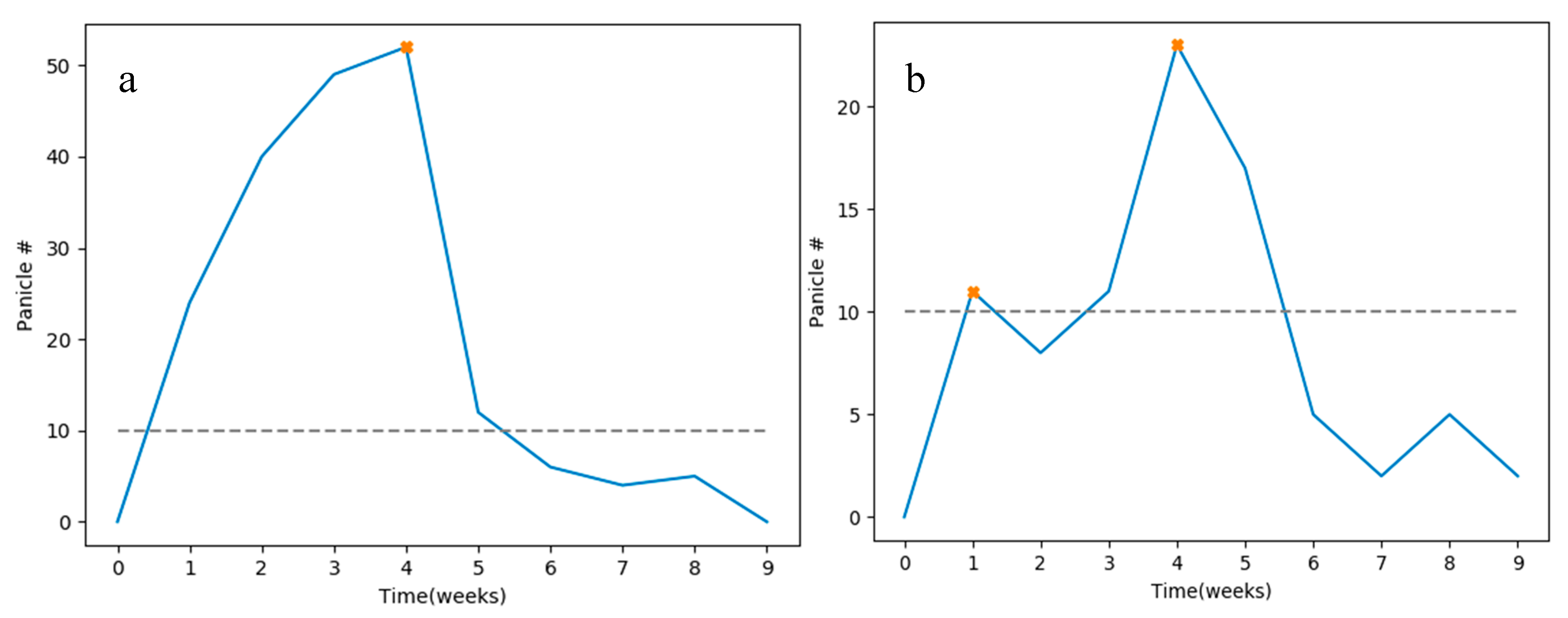
2.4. Estimation of Peak of Flowering

Repeated (weekly) orchard imaging provided a time course of panicle number by week. The signal.find_peaks function from Scipy (www.scipy.org) packages was used to find peaks in the panicle numbers per tree side. Peak properties were specified as height = 10 and distance = 2. Height determines the minimum height of the peak which refers to the minimum number of panicles to consider as a peak. This parameter helps to filter noise (insignificant small peaks) in the signal. Distance determines the minimum horizontal distance in samples between neighbouring peaks.

3. Results

3.1. Segmentation Method

The pixel-segmentation method of [21] differentiates pixels associated to panicles from background based on fixed values of colour thresholding. In poorly illuminated areas of images, panicles were not detected (false negative); while in some images, parts of the tree such as branches or brownish/yellowish leaves were incorrectly classified as flower pixels. Two example images are presented, processed using the segmentation [21] and deep learning R²CNN methods (Figure 4).

Flowering intensity (ratio of panicle pixels to the canopy pixels) was assessed following the method of [21] and correlated to the panicle counts per tree made using the R²CNN(-rotated) method, for all 994 trees (1988 images) of an orchard for each of seven consecutive weeks (

Table 3. Flowering intensity level per tree from pixel segmentation method and Y stage or all stages panicle counts, respectively, from the R²CNN(-rotated) method, and the average ratio of stage Y to total panicle count per image, for each week (n = 1988).

Week	1 16 Aug	2 23 Aug	3 30 Aug	4 6 Sep	5 13 Sep	6 20 Sep	7 27 Sept
(Stage Y) R2	0.903	0.896	0.892	0.788	0.853	0.871	0.708
(Stage X + Y) R2	0.914	0.900	0.777	0.496	0.791	0.846	0.671
(Stage X + Y + Z) R2	0.898	0.865	0.825	0.579	0.254	0.357	0.327
Ratio of stage Y to total panicle count	0.376	0.390	0.395	0.361	0.416	0.320	0.147

). Better correlation was obtained between the stage Y panicle counts rather than the total panicle count in the last two weeks, as the proportion of stage Y panicles changed (Table 3).

3.2. Deep Learning Methods

An example of one image processed with the three methods of MangoYOLO-rotated, R²CNN(-rotated) and R²CNN-upright is given as Figure 5.

The Root Mean Square Error (RMSE) for estimates of total panicle count per tree of the validation set was lowest with the YOLOv3-rotated method, while the lowest RMSE for count of stages X, Y and Z was achieved with the MangoYOLO-rotated and R²CNN-rotated methods (

Table 4. Stage detection results on the validation set using three methods. RMSE refers to a comparison with ground truth assessments of panicles per image. All values refer to number of panicles per tree image. Best results for a given metric and panicle stage are shown in bold.

	Ground Truth				R2CNN(-Rotated)				R2CNN-Upright				MangoYOLO(-Upright)				MangoYOLO-Rotated				YOLOv3-Rotated
Wk.	X	Y	Z	total	X	Y	Z	total	X	Y	Z	total	X	Y	Z	total	X	Y	Z	total	X	Y	Z	total
6	1	37	72	110	1	27	64	92	1	30	46	77	0	27	69	96	0	36	73	109	0	25	100	125
5	13	67	42	122	9	54	36	99	11	41	29	81	0	48	23	71	3	65	22	90	0	67	40	107
4	28	91	8	127	9	62	15	86	22	53	7	82	16	73	11	100	24	78	6	108	11	75	16	102
3	28	69	0	97	16	49	5	70	22	46	0	68	21	57	0	78	24	65	0	89	22	60	1	83
2	46	28	0	74	38	21	1	60	36	17	0	53	43	25	0	68	45	21	0	66	39	23	0	62
1	51	24	0	75	36	16	0	52	43	18	0	61	55	18	0	73	54	17	0	71	54	20	0	74
RMSE					11.6	16.4	5.4	25.8	6.3	21.8	11.8	32.3	8.0	12.7	7.9	25.6	4.9	6.9	8.2	16.0	9.6	9.3	11.9	15.4
Bias					−9.7	−14.5	−1.7	−24.3	−5.3	−18.5	−6.7	−30.5	−5.3	−11.3	−3.2	−19.8	−2.8	−5.7	−3.5	−12.0	−6.8	−7.7	+5.8	−8.7
Average Precision1					56.3	62.0	69.3	62.5	80.8	64.8	67.2	70.9	74.1	76.7	65.6	72.2	68.7	78.1	60.5	69.1	65.4	74.0	55.4	65.0
F12					69.6	75.6	75.7	74.0	89.4	78.7	80.4	82.0	77.8	77.8	71.4	76.5	75.4	79.0	69.5	76.1	76.5	77.1	67.2	74.9

¹ mAP is presented in ‘Total’ column; ² Weighted F1 is presented in ‘Total’ column.

). Low RMSE values were associated with low bias values. RMSE and bias were generally lower with use of rotated compared to upright bounding boxes for both YOLO and R²CNN methods (Table 4). The highest mean average precision and Weighted F1 score was obtained with MangoYOLO and R²CNN-upright models respectively (Table 4).

YOLO and R²CNN methods were also used in prediction of the test set images (two images per tree), collected from a different orchard, cultivar and camera to the calibration set (

Table 5. Comparison of panicle assessment methods on the test image set (from [21]) in terms of the R² and RMSE between machine vision panicle (sum of two sides of a tree) count on images (two per tree) and in-field human counts of panicles per tree.

Detection Method	R2	RMSE	Bias
R2CNN(-rotated)	0.81	91.9	−72.2
R2CNN-upright	0.76	93.2	−72.4
MangoYOLO(-upright)	0.86	50.7	−30.3
MangoYOLO-rotated	0.80	35.6	−6.4
YOLOv3-rotated	0.83	53.5	−33.6
Faster R-CNN [21]	0.78	-	-

, Figure 6). Predicted counts were compared to human counts of panicle stages per tree. The MangoYOLO-rotated method achieved the lowest RMSE and bias of the five methods, while the MangoYOLO(-upright) method returned the highest R² but suffered a high bias (Table 5). The R²CNN-upright model returned a lower R² than the base R²CNN(-rotated) model. The R²CNN-upright model result was similar to that reported by [21] for a Faster R-CNN (VGG-16) method (which uses upright boxes) for the same trees from test set (Table 2).

4. Discussion

4.1. Method Comparison

4.1.1. Pixel Segmentation

The pixel-segmentation method of [21] outputs the total flower and canopy-like pixels and does not provide an estimation of the number of panicles. A correlation was obtained between flowering intensity values and panicle counts, consistent with the report of [21]. However, pixel number per panicle varies with each stage of panicle development, and so confounds the number with the developmental stage. A stronger correlation between flowering intensity and panicle count is expected when all the panicles are at the same stage of development.

The pixel segmentation method also uses a fixed colour threshold range, but colour of panicles and canopy may vary between cultivars and with growing conditions, resulting in false positives and negatives. Use of the segmentation method was therefore discontinued in favour of a deep learning method for object detection, echoing the advice of [12].

4.1.2. Defining Flowering Stages

Mango panicle development is typically described in terms of eight stages: quiescent bud, bud swelling, inflorescence axis elongation, inflorescence sprout, flower opening and inflorescence branching, well-developed inflorescence, and inflorescence starting to set fruit [26]. The early stages are difficult to differentiate from vegetative structures at a distance, and thus, the classification of these stages was not attempted. Initially a four-stage classification was attempted, adding an early stage of development, but the level of uncertainty in the human labelling of the images was high (data not shown). Even with the three-class model, there was uncertainty in annotation, between late X-stage and early Y-stage panicles and late Y-stage and early Z-stage panicles. This uncertainty will adversely affect the classification accuracy of the trained models on the development stage, but it will not affect the model estimate of total panicle number. Figure 7 and Figure 8 illustrate misclassification and the ambiguous classification of panicle stages.

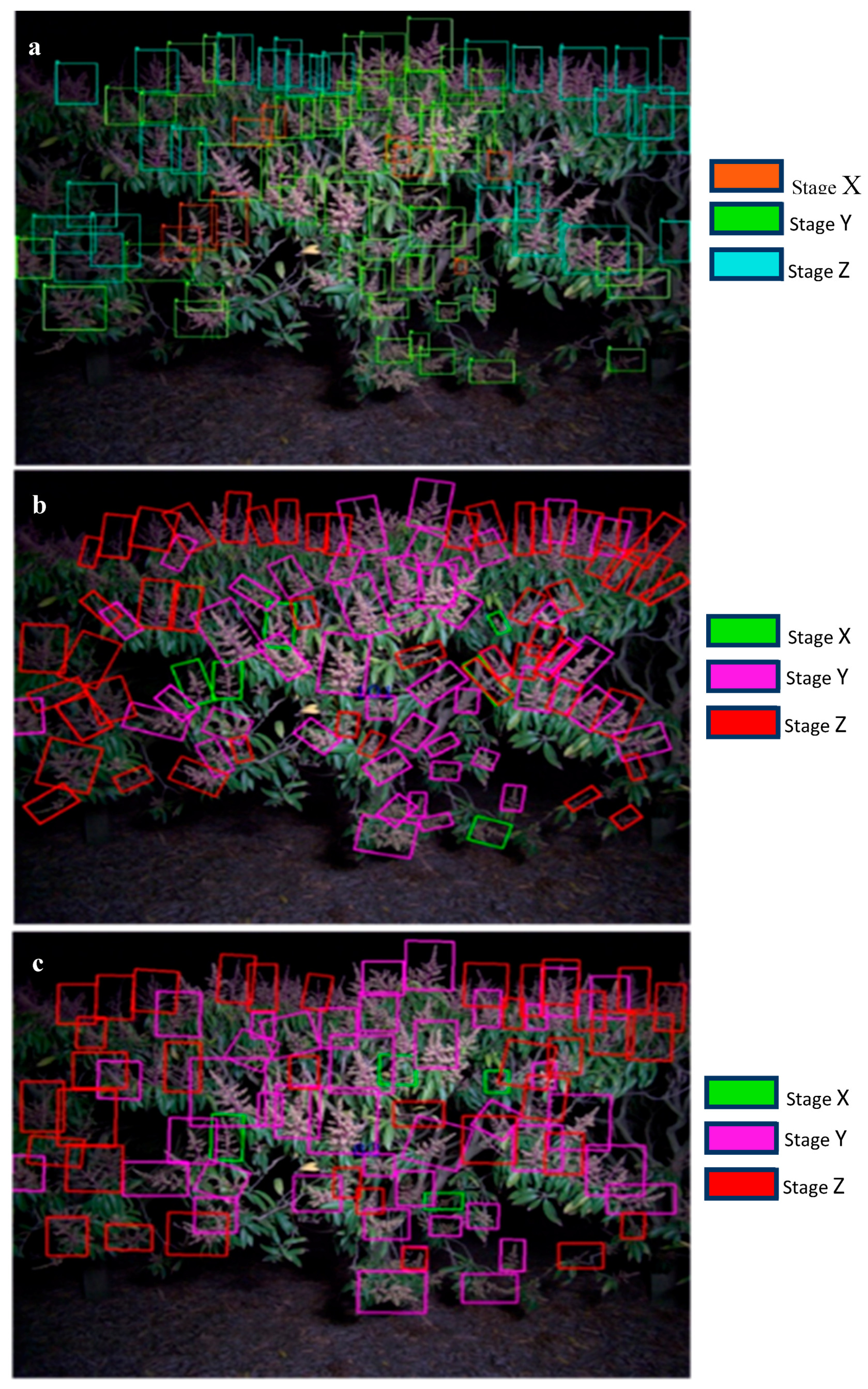
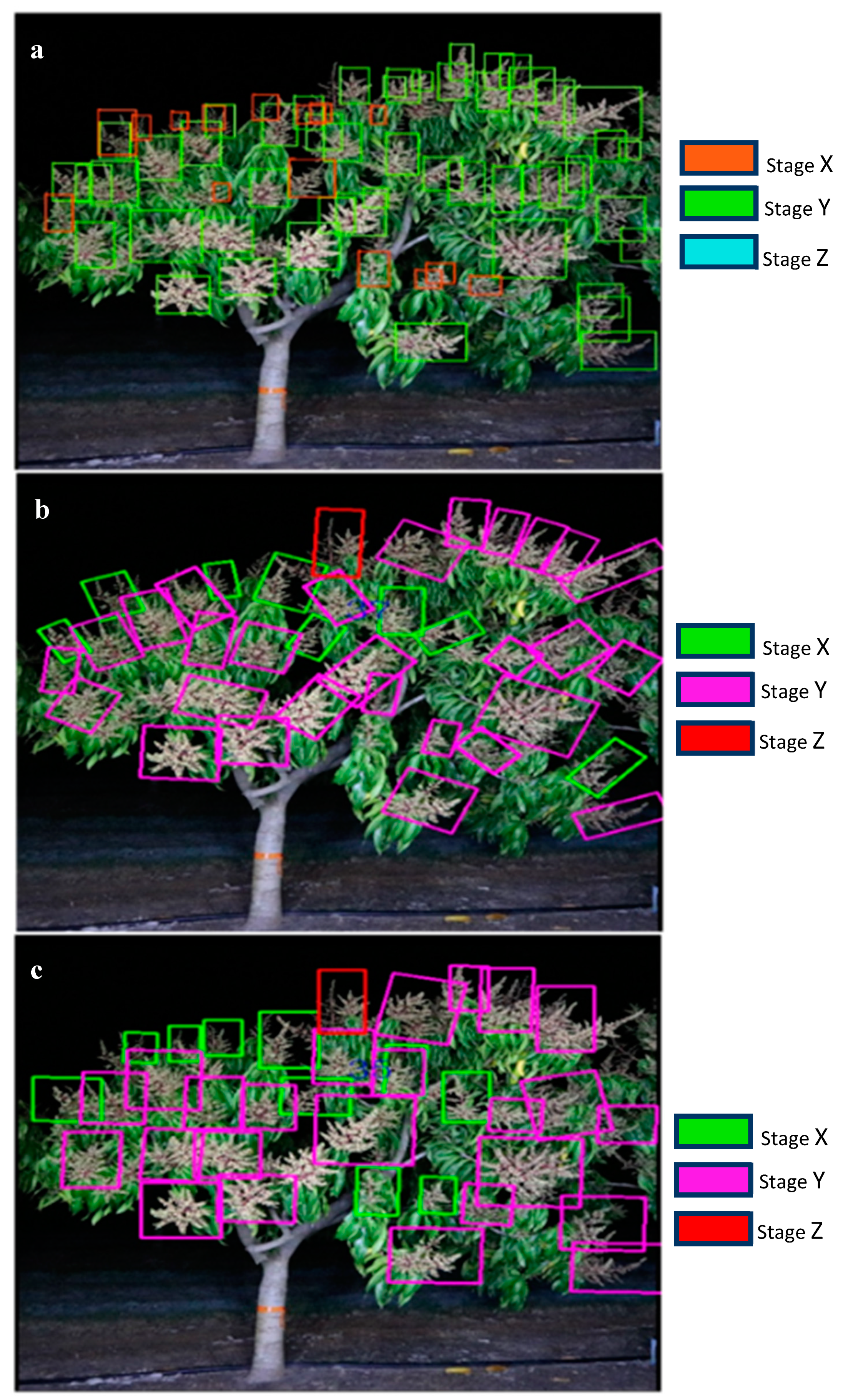
4.1.3. Deep Learning Methods: Use of Rotated Bounding Boxes

R²CNN(-rotated) is a Faster R-CNN framework with the added capability of training on rotated objects (bounding boxes). It was hypothesised that that use of rotated bounding boxes in training and prediction would improve results for panicle detection.

Models trained using image rotation and rotated bounding boxes produced numbers closer to the total panicle count per image, i.e., showed lower bias (Table 4). However, lower mAP and average weighted F1-scores for the rotated models suggest that there was more error in the classification of detected panicles compared to the models trained with the upright bounding box (Table 4). This result indicated that rotated models were better in detecting panicles of different orientations and suited for applications involving a single class; for example, for the task of detecting and counting panicles. However, models for classifying panicles to different classes did not benefit from this approach. Thus, upright models are recommended for applications involving multi-class classification.

We conclude that there was no benefit from use of random panicle rotation as a data augmentation technique for panicle stages classification.

4.1.4. Deep Learning Methods: A Comparison

The five methods (MangoYOLO(-upright), MangoYOLO-rotated, YOLOv3-rotated, R²CNN(-rotated) and R²CNN-upright) ranked differently in terms of RMSE, bias, Precision and F1 score. Such differences are expected, given the difference in calculation of these metrics. RMSE is a ‘gross’ metric compared to Precision and F1 score, as false negatives can be offset by false positive detections to yield a low RMSE metric. Therefore, model performance was primarily assessed on the mAP and F1 evaluation metrics (Table 5).

As a rule of thumb, a deeper CNN can yield superior prediction accuracy. However, performance is also related to architecture (connecting layers, etc.) as well as depth [27]. A comparison of the R²CNN-upright method with its deeper CNN classifier (ResNet101) to the single- shot MangoYOLO(-upright) method is useful in this respect. In the validation exercise, the R²CNN-upright method produced a higher weighted F1-score, but a lower mAP score compared to the MangoYOLO(-upright) method (Table 4). This outcome suggests that the YOLO method suffered from lower recall rates.

The performance of the deeper single shot detector, YOLOv3, was also compared to that of the MangoYOLO method. The better results (mAP and F1-score) of the MangoYOLO method were consistent with previous results in fruit detection [12], and suggest that the MangoYOLO architecture is better suited to this application than that of YOLOv3.

The YOLOv3-rotated model returned the lowest bias and RMSE for count of panicles per image, but R²CNN-upright returned the highest F1 score (Table 4 and Figure 5) and the MangoYOLO(-upright) model achieved the highest mAP score (Table 4). For the test exercise, the standout result was a low bias and associated low RMSE for the MangoYOLO-rotated model (Table 5).

Panicle image size (in pixels) can vary due to variation in camera to tree distance or use of different camera lens. YOLO models can be robust for such conditions, as the YOLO object detection framework provides multiscale image training as a part of data augmentation. Other data augmentation techniques such as random rotation and random change in hue, saturation and exposure of training samples provides robustness for the YOLO model to deal with variation in lighting conditions and cultivars. In comparison, R²CNN like Faster R-CNN does not support multiscale training, and the only data augmentation during training provided is image flipping (horizontal and vertical flips). Therefore, the YOLO method of object detection is recommended for applications similar to those considered in the current study.

The speed of classification by YOLO and R²CNN methods could not be compared because R²CNN supports standard CNN classifier architectures such as ResNet and MobileNet while YOLO uses a custom CNN classifier architecture, with no support for standard CNN classifiers. It is expected, however, that YOLO will process images faster than R²CNN as the object detection framework of YOLO uses a single-stage detection technique, in comparison with the dual-stage detection technique of R²CNN. In [12], researchers documented speed and memory requirement comparisons of several deep learning object detection frameworks. For example, it took 10, 25 and 67 ms for mango fruit detection on tree images (512 × 512 pixels)—requiring 873, 2097 and 1759 Mb of GPU memory for MangoYOLO, YOLOv3 and Faster-RCNN (VGG16) models, respectively.

4.2. Applications

One of the challenges in precision agriculture is the display and interpretation of large data sets in a form useful to the farm manager, i.e., an appropriate decision-support tool for farm management is required. Thus, the presentation of data on panicle count by stage of development for every tree in an orchard requires consideration. A key assessment is the timing of flowering, which can be used in conjunction with calendar days or thermal time to estimate harvest date. This is useful for planning harvest resourcing. Inaccurate harvest timing estimation will result either in harvests of less mature fruit, resulting in lowered eating quality, or over-mature fruit, with reduced postharvest life.

For example, panicle stage data can be presented on an individual tree basis by week as a line graph (Figure 9). This figure enables the identification of early flowering areas in one row of an orchard, but it does not scale well to consideration of an entire orchard block.

Data can also be presented on a farm map, using a colour scale to display values, per week of imaging (Figure 10) using the web-app described by [28], which allows display of the individual images associated with each tree.

Alternatively, data can be summarised for an orchard block, with a tally of panicles by development stage by week (Figure 11). In the example data, there was a shift in developmental stage from stage X to Y to Z over the monitored period—as expected given panicle development. A peak in total count occurred at week 5. This profile can be interpreted as a single sustained flowering event maintained over four weeks (weeks 1 to 5).

In another approach, the timing of the peak in panicle number per tree can be assessed for individual trees given a time course of images and use of a peak detection routine (Figure 12).

A display of the number of trees with peaks in X stage panicle count each week can be displayed, to give a sense of when the orchard generally has a peak flowering event. For example, of 1986 images of 993 trees in orchard A, 168 tree-sides (8%) displayed two flowering events (peaks in stage X) (Figure 13). The first flowering event occurred in the first two weeks of imaging while another peak flowering event occurred on the fourth week. This information on major flowering events can be coupled to temperature records to provide an estimated harvest maturity time based on thermal time [28]. If the events are sufficiently large and temporally separated, the grower can consider these as separate harvest populations.

Alternatively, data can be presented on a farm map for the selective display of the spread of panicles per week of imaging (Figure 14). In this software [21], an individual tree can be selected to display the flowering level, tree image, image capture date and tree identity (not shown).

5. Conclusions

A method is presented in this paper for the estimation of panicle number and stage of development. A method is also presented for the detection of a peak flowering event in a time series. This gives a point from which to calculate a thermal or calendar time to fruit maturation, a critical estimate for harvest management. The extent of flowering also provides an index to potential crop yield (fruit number) although in previous studies we have shown a poor correlation between the number of panicles and the fruit numbers (i.e., variable and high flower and fruit drop). The spatial information on the spread of flowering also provide growers with wealth of information for agronomic treatments.

Deep learning methods can automatically learn the useful features required in an application. For panicle detection, this is likely to involve colour and shape patterns. Similar to that demonstrated by [12] for the fruit detection application, a deep learning method was demonstrated to generalize in terms of application to an orchard of different cultivar, growing conditions and canopy architecture, and also to images acquired with a different camera to that used for the training images. Similarly, [18] reported that a deep learning FCN trained on apple flower images was able to generalize well for peach and pear flower detection, and to operate across camera hardware. The use of deep learning models over traditional segmentation techniques for the application of panicle developmental stage detection is thus confirmed.

In addition to total panicle counts, classification of panicle into several developmental stages was achieved. This is an important step in allowing the extraction of information on the time-spread of flowering, and thus of the future harvest. Counts of panicles in stage X over time were used for estimating the timing of peak flowering events. Counts of panicles in stage Y demonstrated the highest correlation with the flower intensity level per tree.

There has been continuous evolution of CNN architectures in terms of increased depth (number of layers) for better performance, but recent improvements in the representational capacity of deep CNNs has been attributed to the restructuring of processing units (e.g., having multiple paths and connections) rather than just increasing depth [27]. The better performance of MangoYOLO compared to deeper CNN architecture of YOLOv3 for panicle detection is consistent to the report of [12] for fruit detection, and can be ascribed to CNN design considerations.

The YOLO method of object detection is recommended for total panicle classification and count, and similar applications. The procedure offers a large set of data augmentation features (e.g., image rotation, HSV channel values, jitter, image scale etc.) that can be specified by the user to create robust models. Moreover, YOLO is a single shot detection technique and provides a faster detection rate compared to two-stage detection methods (e.g., Faster R-CNN) which allows YOLO models to be operated in real-time.

The use of rotated training images improved the detection of panicles and thus this approach is recommended for applications that require counting the instances of objects in natural scenes and having different orientations. However, for applications that require more emphasis on the multi-class classification of the objects, it is recommended to use upright bounding boxes.

There have been several publications on machine-vision-based detection and crop load estimation for tree fruit crops, but relatively few reports of in-field tree crop flower assessment especially in terms of developmental stage. There has been even less attention given to the presentation and management of such data. The flower peak detection and display options presented in the current study should prompt further work in this field.

References

1. Aggelopoulou, A.; Bochtis, D.; Fountas, S.; Swain, K.C.; Gemtos, T.; Nanos, G. Yield prediction in apple orchards based on image processing. Precis. Agric. 2011, 12, 448–456. [Google Scholar] [CrossRef]
2. Dorj, U.-O.; Lee, M. A new method for tangerine tree flower recognition. In Computer Applications for Bio-Technology, Multimedia, and Ubiquitous City; Springer: Heidelberg, Germany, 2012; pp. 49–56. [Google Scholar]
3. Horton, R.; Cano, E.; Bulanon, D.; Fallahi, E. Peach flower monitoring using aerial multispectral imaging. J. Imaging 2017, 3, 2. [Google Scholar] [CrossRef]
4. Hočevar, M.; Širok, B.; Godeša, T.; Stopar, M. Flowering estimation in apple orchards by image analysis. Precis. Agric. 2014, 15, 466–478. [Google Scholar] [CrossRef]
5. Oppenheim, D.; Edan, Y.; Shani, G. Detecting Tomato Flowers in Greenhouses Using Computer Vision. Int. J. Comput. Electr. Autom. Control Inform. Eng. 2017, 11, 104–109. [Google Scholar]
6. Underwood, J.P.; Hung, C.; Whelan, B.; Sukkarieh, S. Mapping almond orchard canopy volume, flowers, fruit and yield using lidar and vision sensors. Comput. Electron. Agric. 2016, 130, 83–96. [Google Scholar] [CrossRef]
7. Diago, M.P.; Sanz-Garcia, A.; Millan, B.; Blasco, J.; Tardaguila, J. Assessment of flower number per inflorescence in grapevine by image analysis under field conditions. J. Sci. Food Agric. 2014, 94, 1981–1987. [Google Scholar] [CrossRef]
8. Guo, W.; Fukatsu, T.; Ninomiya, S. Automated characterization of flowering dynamics in rice using field-acquired time-series RGB images. Plant Methods 2015, 11, 7–23. [Google Scholar] [CrossRef] [Green Version]
9. Kamilaris, A.; Prenafeta-Boldú, F.X. Deep learning in agriculture: A survey. Comput. Electron. Agric. 2018, 147, 70–90. [Google Scholar] [CrossRef] [Green Version]
10. Koirala, A.; Walsh, K.B.; Wang, Z.; McCarthy, C. Deep learning—Method overview and review of use for fruit detection and yield estimation. Comput. Electron. Agric. 2019, 162, 219–234. [Google Scholar] [CrossRef]
11. Gongal, A.; Amatya, S.; Karkee, M.; Zhang, Q.; Lewis, K. Sensors and systems for fruit detection and localization: A review. Comput. Electron. Agric. 2015, 116, 8–19. [Google Scholar] [CrossRef]
12. Koirala, A.; Wang, Z.; Walsh, K.; McCarthy, C. Deep learning for real-time fruit detection and orchard fruit load estimation: Benchmarking of ‘MangoYOLO’. Precis. Agric. 2019, 20, 1107–1135. [Google Scholar] [CrossRef]
13. Redmon, J.; Divvala, S.; Girshick, R.; Farhadi, A. You only look once: Unified, real-time object detection. In Proceedings of Proceedings of the IEEE Computer Society Conference on Computer Vision and Pattern Recognition, Honolulu, HI, USA, 21–26 July 2017; pp. 779–788. [Google Scholar]
14. Redmon, J.; Farhadi, A. YOLOv3: An Incremental Improvement. Available online: https://arxiv.org/abs/1706.09579 (Accessed on 10 December 2019).
15. Dias, P.A.; Tabb, A.; Medeiros, H. Apple flower detection using deep convolutional networks. Comput. Ind. 2018, 99, 17–28. [Google Scholar] [CrossRef] [Green Version]
16. Zeiler, M.D.; Fergus, R. Visualizing and Understanding Convolutional Networks; Springer: Basel, Switzerland, 2014; pp. 818–833. [Google Scholar]
17. Cortes, C.; Vapnik, V. Support-vector networks. Mach. Learn. 1995, 20, 273–297. [Google Scholar] [CrossRef]
18. Dias, P.A.; Tabb, A.; Medeiros, H. Multispecies Fruit Flower Detection Using a Refined Semantic Segmentation Network. IEEE Robot. Autom. Lett. 2018, 3, 3003–3010. [Google Scholar] [CrossRef] [Green Version]
19. Chen, L.; Papandreou, G.; Kokkinos, I.; Murphy, K.; Yuille, A.L. DeepLab: Semantic Image Segmentation with Deep Convolutional Nets, Atrous Convolution, and Fully Connected CRFs. IEEE Trans. Pattern Anal. 2018, 40, 834–848. [Google Scholar] [CrossRef] [PubMed]
20. Wang, Z.; Verma, B.; Walsh, K.B.; Subedi, P.; Koirala, A. Automated mango flowering assessment via refinement segmentation. In Proceedings of the International Conference on Image and Vision Computing New Zealand (IVCNZ), Palmerston North, New Zealand, 21–22 Novermber 2016; pp. 1–6. [Google Scholar]
21. Wang, Z.; Underwood, J.; Walsh, K.B. Machine vision assessment of mango orchard flowering. Comput. Electron. Agric. 2018, 151, 501–511. [Google Scholar] [CrossRef]
22. Ren, S.; He, K.; Girshick, R.; Sun, J. Faster R-CNN: Towards real-time object detection with region proposal networks. IEEE Trans. Pattern. Anal. 2017, 39, 91–99. [Google Scholar] [CrossRef] [PubMed] [Green Version]
23. Jiang, Y.; Zhu, X.; Wang, X.; Yang, S.; Li, W.; Wang, H.; Fu, P.; Luo, Z. R2CNN: Rotational Region CNN for Orientation Robust Scene Text Detection. Available online: https://arxiv.org/abs/1901.06032 (accessed on 10 December 2019).
24. OpenCV. OpenCV Library. Available online: http://opencv.org/ (accessed on 4 November 2019).
25. Redmon, J.; Farhadi, A. YOLO9000: Better, Faster, Stronger. In Proceedings of Proceedings of the IEEE Conference on Computer Vision and Pattern Recognition, Honolulu, HI, USA, 21–26 July 2017; pp. 7263–7271. [Google Scholar]
26. Yeshitela, T.; Robbertse, P.; Stassen, P. The impact of panicle and shoot pruning on inflorescence and yield related developments in some mango cultivars. J. Appl. Hort. 2003, 5, 69–75. [Google Scholar]
27. Khan, A.; Sohail, A.; Zahoora, U.; Qureshi, A.S. A Survey of the Recent Architectures of Deep Convolutional Neural Networks. Available online: https://arxiv.org/abs/1901.06032 (accessed on 10 December 2019).
28. Walsh, K.; Wang, Z. Monitoring fruit quality and quantity in mangoes. In Achieving Sustainable Cultivation of Mangoes; Galán Saúco, V., Lu, P., Eds.; Burleigh Dodds Science Publishing: Cambridge, UK, 2018; pp. 313–338. [Google Scholar]
Figure 1. (a) Original image, (b) upright bounding box and (c) rotated bounding box.
Agronomy 10 00143 g001
Figure 2. Examples for stages X to Z, by rows.
Agronomy 10 00143 g002aAgronomy 10 00143 g002b
Figure 3. Visualization of ground truth bounding box original (rotated) red colour for R2CNN training and transformed (upright) blue colour for MangoYOLO training.
Agronomy 10 00143 g003
Figure 4. Pixel segmentation (a,c) and deep learning R2CNN(-rotated) (b,d) results for the same images. Flowers in the dark background did not segment properly (a), and branches and leaves were erroneously segmented as flower pixels (c).
Agronomy 10 00143 g004
Figure 5. Image processed with three methods for panicle stage detection. (a) MangoYOLO-rotated method. Orange, green and blue coloured boxes represent panicle stages X, Y and Z respectively. (b) R2CNN(-rotated) and (c) R2CNN-upright methods, respectively. Green, pink and red coloured boxes represent panicle classes of X, Y and Z, respectively.
Agronomy 10 00143 g005
Figure 6. Images of panicle stage detection on Canon images of [21]. (a) MangoYOLO(-upright) method: orange, green and blue coloured boxes represent panicle stages X, Y and Z respectively. (b) R2CNN(-rotated) and (c) R2CNN-upright methods, respectively: green, pink and red coloured boxes represent panicle classes of X, Y and Z, respectively.
Agronomy 10 00143 g006
Figure 7. Representative examples of differences in classification from YOLO and R2CNN models. Ground truth and predicted results by YOLO and R2CNN, respectively.
Agronomy 10 00143 g007
Figure 8. Ambiguity in classification. Examples of the panicle stages which the YOLO models predicted to 50% probability for each class. The top (ad) and bottom (eh) panels depict panicles classified to both classes X and Y (a,b,e,f), and Y and Z (c,d,g,h), respectively.
Agronomy 10 00143 g008
Figure 9. Course (weeks 1, 3, 5 and 7) of panicle number by developmental stage per tree for a row of trees.
Agronomy 10 00143 g009
Figure 10. (a) Intensity level and (b) panicle count (using R2CNN(-rotated)) of an orchard with tree rows (994 trees, 1988 images). The colours green, orange and red colour corresponds to low, medium and high flowering levels, per tree with each coloured dot representing the image of one side of a tree. In the top panel the categories are in terms of flower pixels as a percentage of canopy pixels (<10%, 10% to 25% and >25%). In the bottom panel, the categories are in terms of total panicle number (<30, 30 to 70 and >70 panicles per tree image).
Agronomy 10 00143 g010
Figure 11. Flower stages trend analysis across weeks for an orchard.
Agronomy 10 00143 g011
Figure 12. Flowering event detection on stage-X panicle counts for two different trees across 9 weeks of imaging. (a) Single peak and (b) double peaks marked with a coloured dot.
Agronomy 10 00143 g012
Figure 13. (a) Plot displaying the weeks in which a peak flowering event was noted and (b) plot displaying the week of the largest flowering event for 168 trees in which two flowering peaks were recorded.
Agronomy 10 00143 g013
Figure 14. Data of the imaging run of week-1 of Orchard A, in terms of number of panicles at stages (a) X, (b) Y and (c) Z. Dark green, light green, orange and red colours correspond to <30; 30 to 70, 70 to 100 and >100 panicles per tree image.
Agronomy 10 00143 g014