A Method for Estimating Alfalfa (Medicago sativa L.) Forage Yield Based on Remote Sensing Data

Abstract

Alfalfa (Medicago sativa L.) is a widely planted perennial legume forage plant with excellent quality and high yield. In production, it is very important to determine alfalfa growth dynamics and forage yield in a timely and accurate manner. This study focused on inverse algorithms for predicting alfalfa forage yield in large-scale alfalfa production. We carried out forage yield and aboveground biomass (AGB) field surveys at different times in 2022. The correlations among the reflectance of different satellite remote sensing bands, vegetation indices, and alfalfa forage yield/AGB were analyzed, additionally the suitable bands and vegetation indices for alfalfa forage yield inversion algorithms were screened, and the performance of the statistical models and machine learning (ML) algorithms for alfalfa forage yield inversion were comparatively analyzed. The results showed that (1) regarding different harvest times, the alfalfa forage yield inversion model for first-harvest alfalfa had relatively large differences in growth, and the simulation accuracy of the alfalfa forage yield inversion model was higher than that for the other harvest times, with the growth of the second- and third-harvest alfalfa being more homogeneous and the simulation accuracy of the forage yield inversion model being relatively low. (2) In the alfalfa forage yield inversion model based on a single parameter, the moisture-related vegetation indices, such as the global vegetation moisture index (GVMI), normalized difference water index (NDWI) and normalized difference infrared index (NDII), had higher coefficients of correlation with alfalfa forage yield/AGB, and the coefficients of correlation R² values for the first-harvest alfalfa were greater than 0.50, with the NDWI correlation being the best with an R² value of 0.60. (3) For the alfalfa forage yield inversion model constructed with vegetation indices and band reflectance as multiparameter variables, the random forest (RF) and support vector machine (SVM) simulation accuracy was higher than that of the alfalfa forage yield inversion model based on a single parameter; the first-harvest alfalfa R² values based on the multiparameter RF and SVM models were both 0.65, the root mean square errors (RMSEs) were 329.74 g/m² and 332.32 g/m², and the biases were −0.47 g/m² and −2.24 g/m², respectively. The vegetation indices related to plant water content can be considered using a single parameter inversion model for alfalfa forage yield, the vegetation indices and band reflectance can be considered using a multiparameter inversion model for alfalfa forage yield, and ML algorithms are also an optimal choice. The findings in this study can provide technical support for the effective and strategic production management of large-scale alfalfa.

1. Introduction

Alfalfa (Medicago sativa L.), a perennial leguminous forage, is widely cultivated for its excellent quality and high forage yield [1,2,3,4]. In recent years, China’s livestock industry, especially the dairy industry, has been developing rapidly, and the overall demand for alfalfa forage has been increasing [5,6]. In the context of the imbalance between alfalfa forage supply and demand, large-scale, intensive, mechanized, and specialized alfalfa forage production is one of the important methods applied to solve the problem [7,8]. A timely and accurate determination of alfalfa growth dynamics and forage yield is of great significance in large-scale alfalfa forage production management [9]. The traditional estimation of vegetation yield usually relies on manual investigation methods, which are time-consuming and labor-intensive and come with significant difficulties in terms of spatiotemporal dynamic monitoring [10,11,12]. Remote sensing technology enables large-scale synchronous observation with excellent timeliness and indirect contact, making it possible to achieve non-destructive, efficient, and objective dynamic monitoring of plant growth [13,14,15]. Remote sensing technology has played an important role in agricultural production management, mainly for crop distribution and area, growth, yield, disasters, etc. [16,17,18,19,20]. Bolton et al. [21] estimated corn and soybean yields in the central United States using the enhanced vegetation index 2 (EVI2) and normalized difference water index (NDWI) that were calculated using the modified resolution imaging spectroradiometer (MODIS) product. Islam et al. [22] utilized MODIS products by applying a series of data processing techniques and customized machine learning (ML) models and found that the normalized difference vegetation index (NDVI) product relying solely on remote sensing inversion was insufficient for the accurate estimation of crop yield; however, when other meteorological variables were added to the ML model, the estimation accuracy was significantly improved. Fan et al. [23] used Sentinel-2 remote sensing data to calculate 10 vegetation indices by combining the remote sensing data with field survey, meteorological, and terrain data, and constructed an ML model for estimating AGB.

At present, the use of remote sensing technology for vegetation yield estimation focuses mainly on crops such as wheat, corn, and rice and is relatively rare in alfalfa forage yield estimation [24,25]. Kayad et al. [26] used multiple vegetation indices extracted from Landsat images to invert the yield of alfalfa in Saudi Arabia and found a strong correlation between the near-infrared band, soil-adjusted vegetation index (SAVI), NDVI, and alfalfa forage yield. Azadbakht et al. [27] used time series images from Landsat 8 and PROBA-V to establish alfalfa forage yield inversion models through various ML methods using features selected by Gram Schmidt and found that the Gaussian process regression model performed the best. Zhou et al. [28] used multiple satellite remote sensing data such as MODIS and Sentinel-2 to determine the harvest of alfalfa in central Oklahoma and found that integrating multiple optical remote sensing data could improve the temporal resolution, making it more suitable for monitoring alfalfa harvest times and field-scale disturbances. As a perennial forage, alfalfa can be cut multiple times a year. Does the alfalfa harvest number (i.e., first-harvest, second-harvest, third-harvest, etc.) have an impact on the alfalfa forage yield inversion model? Is there saturation in the vegetation indices when estimating alfalfa forage yield? What are the differences in the applicability and accuracy between different inversion algorithms? Answering these questions still requires further research.

This study focused on inversion algorithms for alfalfa forage yield in large-scale production. Field surveys of alfalfa forage yield and AGB in alfalfa from different harvests were conducted, and we carried out alfalfa forage yield and AGB field surveys of different harvests in 2022. The correlations between the reflectance of different satellite remote sensing bands, vegetation indices and alfalfa forage yield/AGB were analyzed, the suitable bands and vegetation indices for alfalfa forage yield inversion algorithms were screened, and the performance of statistical models (exponential function (Exp)) and ML algorithms (linear regression (LR), multiple stepwise regression (SLR), partial least squares regression (PLSR), RF, SVM, and artificial neural network (ANN)) in alfalfa forage yield inversion were comparatively analyzed. The results of this study can provide technical support for the effective and strategic production management of large-scale alfalfa cultivation.

2. Materials and Methods

2.1. Study Area

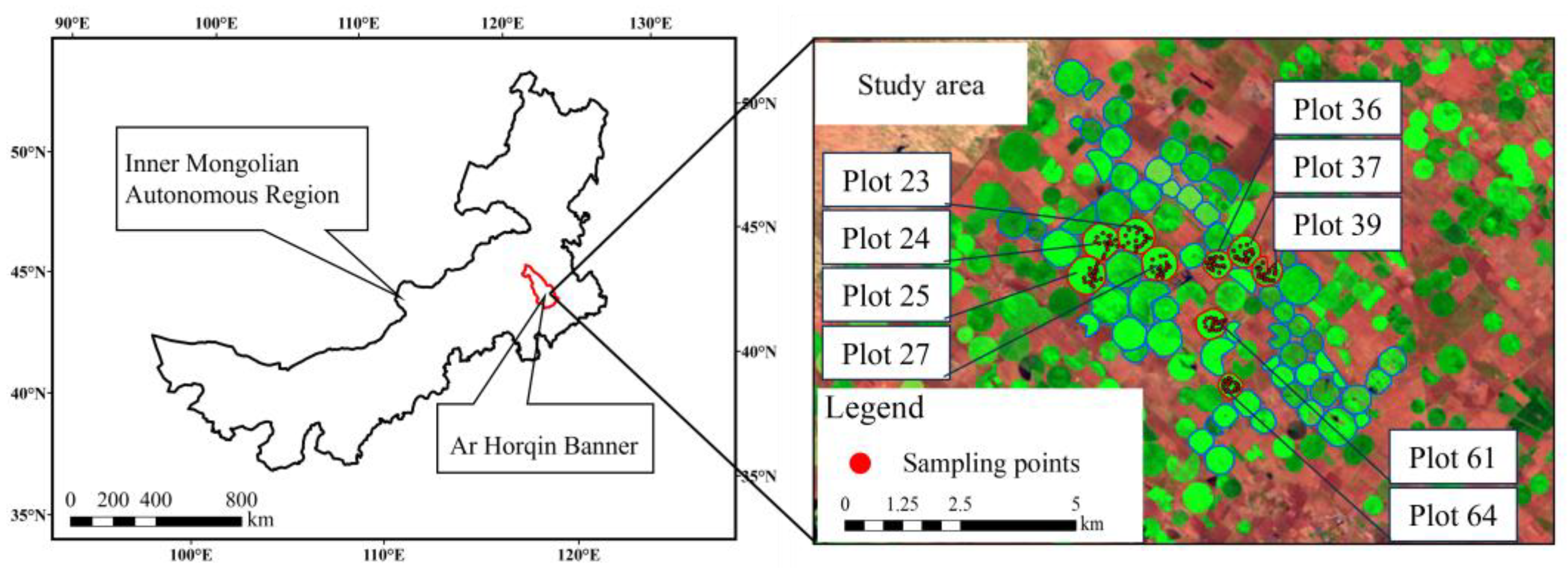
The study area was located in the southern part of Ar Horqin Banner, Chifeng City, Inner Mongolia Autonomous Region, China (Figure 1), which has a temperate continental climate, with an annual average temperature of approximately 6 °C, an extreme maximum temperature above 40 °C, an extreme minimum temperature below −30 °C, and an annual precipitation between 300 and 400 mm. Animal husbandry is the main economic pillar of Ar Horqin Banner, and alfalfa and oats (Avena sativa L.) are the most widely planted forage species. Ar Horqin Banner is also an alfalfa-planting standardization demonstration area.

2.2. Data

2.2.1. Field Survey Data

In this study, 9 alfalfa plots with different growth conditions covering an area of 0.20–0.60 km² were selected. The field survey was conducted from May to August in 2022, and the alfalfa was harvested three times. Notably, the alfalfa AGB is the aboveground biomass of alfalfa plants, and the AGB before the harvest of alfalfa is the alfalfa forage yield. Considering that there may be saturation when using the vegetation indices to invert alfalfa forage yield, the alfalfa AGB was measured between the first- and second-harvest times and between the second and third-harvest times when the alfalfa AGB was low. The alfalfa forage yield and AGB were measured five times, and seven 1 m × 1 m sampling squares were set up in each sampling plot using portable GPS to record latitude and longitude. Then, the aboveground parts of alfalfa plants in the sampling plots were cut off, and the fresh AGB was weighed and brought back to the laboratory. The samples were placed in an oven at 105 °C for 30 min, dried at 65 °C until reaching a constant weight, and then weighed to determine the dry weight. A total of 314 valid sampling points (Figure 1) were obtained.

2.2.2. Satellite Remote Sensing Data

MODIS surface reflectance products (MOD09GQ, 250 m spatial resolution) were used to study the alfalfa dynamic growth characteristics, which were obtained from the National Aeronautics and Space Administration (NASA; https://ladsweb.modaps.eosdis.nasa.gov, accessed on 12 November 2022), and the MODIS images were reprojected and converted into Georeferenced Tagged Image File (GeoTIFF) with the HDF-EOS to GeoTIFF Conversion Tool (HEG). Sentinel-2 MSI Level-2A products (20 m spatial resolution) were used to study the inversion model of alfalfa forage yield, which were obtained from the European Space Agency (ESA; https://scihub.copernicus.eu, accessed on 12 November 2022). The remote sensing image processing and vegetation index calculations were implemented using ENVI 5.3 software.

2.3. Methods

2.3.1. Vegetation Indices

In this study, 10 vegetation indices (

Table 1. Vegetation index calculation formula.

Index Name	Formula	Sentinel Bands	Reference
NDVI	$\frac{\mathrm{N}\mathrm{I}\mathrm{R}-\mathrm{R}\mathrm{E}\mathrm{D}}{\mathrm{N}\mathrm{I}\mathrm{R}+\mathrm{R}\mathrm{E}\mathrm{D}}$	4, 8A	[29]
EVI	$\frac{2.5\times \left(\mathrm{N}\mathrm{I}\mathrm{R}-\mathrm{R}\mathrm{E}\mathrm{D}\right)}{\mathrm{N}\mathrm{I}\mathrm{R}+6\mathrm{R}\mathrm{E}\mathrm{D}-7.5\mathrm{B}\mathrm{L}\mathrm{U}\mathrm{E}+1}$	2, 4, 8A	[30]
NDWI	$\frac{\mathrm{G}\mathrm{R}\mathrm{E}\mathrm{E}\mathrm{N}-\mathrm{N}\mathrm{I}\mathrm{R}}{\mathrm{G}\mathrm{R}\mathrm{E}\mathrm{E}\mathrm{N}+\mathrm{N}\mathrm{I}\mathrm{R}}$	3, 8A	[31]
NDPI	$\frac{\mathrm{N}\mathrm{I}\mathrm{R}-\left(0.74\times \mathrm{R}\mathrm{E}\mathrm{D}+0.26\times \mathrm{S}\mathrm{W}\mathrm{I}\mathrm{R}\right)}{\mathrm{N}\mathrm{I}\mathrm{R}+\left(0.74\times \mathrm{R}\mathrm{E}\mathrm{D}+0.26\times \mathrm{S}\mathrm{W}\mathrm{I}\mathrm{R}\right)}$	8A, 11	[32]
SAVI	$\left(1+\mathrm{L}\right)\frac{\mathrm{N}\mathrm{I}\mathrm{R}-\mathrm{R}\mathrm{E}\mathrm{D}}{\mathrm{N}\mathrm{I}\mathrm{R}+\mathrm{R}\mathrm{E}\mathrm{D}+\mathrm{L}}\mathrm{L}=0.25$	4, 8A	[33]
MSAVI	$\frac{1}{2}\times \left[\left(2\times \mathrm{N}\mathrm{I}\mathrm{R}+1\right)-\left(\sqrt{{\left(2\times \mathrm{N}\mathrm{I}\mathrm{R}+1\right)}^2-8\times \left(\mathrm{N}\mathrm{I}\mathrm{R}-\mathrm{R}\mathrm{E}\mathrm{D}\right)}\right)\right]$	4, 8A	[34]
NDII	$\frac{\mathrm{N}\mathrm{I}\mathrm{R}-\mathrm{S}\mathrm{W}\mathrm{I}\mathrm{R}1}{\mathrm{N}\mathrm{I}\mathrm{R}+\mathrm{S}\mathrm{W}\mathrm{I}\mathrm{R}1}$	8A, 11	[35]
GVMI	$\frac{\left(\mathrm{N}\mathrm{I}\mathrm{R}+0.1\right)-\left(\mathrm{S}\mathrm{W}\mathrm{I}\mathrm{R}+0.02\right)}{\left(\mathrm{N}\mathrm{I}\mathrm{R}+0.1\right)+\left(\mathrm{S}\mathrm{W}\mathrm{I}\mathrm{R}+0.02\right)}$	8A, 11	[36]
NDVIRE	$\frac{\mathrm{N}\mathrm{I}\mathrm{R}-\mathrm{R}\mathrm{E}1}{\mathrm{N}\mathrm{I}\mathrm{R}+\mathrm{R}\mathrm{E}1}$	8A, 5	[37]
ND705	$\frac{\mathrm{R}\mathrm{E}2-\mathrm{R}\mathrm{E}1}{\mathrm{R}\mathrm{E}2+\mathrm{R}\mathrm{E}1}$	5, 6	[38]

Note: GREEN, BLUE, RED, NIR, RE, RE1, RE2, and SWIR are the surface reflectance values for green, blue, red, near-infrared, red edge 1 (center wavelength is 705 nm), red edge 2 (center wavelength is 740 nm) and shortwave infrared waves, respectively.

) were selected, including the red band, green band, blue band, near-infrared band, shortwave infrared band, and red edge. These vegetation indices can be divided into multiple types, some of which are sensitive to water, such as the NDWI; those that can enhance vegetation information, such as the enhanced vegetation index (EVI); and those that can reduce the influence of the soil background, such as the SAVI and modified soil adjusted vegetation index (MSAVI). There are widely used indices, such as the NDVI; some are more sensitive to vegetation condition change, such as the normalized difference red-edge index (NDVIRE) and red-edge normalized difference red-edge index (ND705); and there are newer vegetation indices, such as the normalized difference phenology index (NDPI).

2.3.2. Alfalfa Forage Yield Inversion Model

The alfalfa forage yield inversion model was constructed by remote sensing, which used the alfalfa forage yield field survey data three times, the AGB data two times between different harvest times, and Sentinel-2 MSI image data. The main research content included the following:

① The correlations among reflectance in different bands, vegetation indices, and alfalfa forage yield/AGB

Ten vegetation indices were calculated based on the reflectance of different bands of Sentinel-2 MSI images, and the correlation between the reflectance and alfalfa forage yield/AGB was analyzed. This included the first-harvest alfalfa forage yield, the second-harvest alfalfa forage yield, the third-harvest alfalfa forage yield, the AGB between the first- and second-harvest time points, and the AGB between the second- and third-harvest time points.

② Alfalfa forage yield inversion model based on a single parameter

A single-parameter alfalfa forage yield inversion model was constructed by the selected vegetation indices using the Exp, LR, RF, SVM, and ANN algorithms.

③ Alfalfa forage yield inversion model based on multiple parameters

The multiple-parameter alfalfa forage yield inversion model was constructed by the different reflectance bands and vegetation indices using the SLR, PLSR, RF, SVM, and ANN algorithms.

④ Model simulation and accuracy evaluation

In this study, field survey data from 2022 was used for model training and accuracy evaluation. All AGB data from the first- to the second-harvest and the second- to the third-harvest; moreover, 70% of the first-harvest, second-harvest, and third-harvest alfalfa forage yield data were used as training sets, and 30% of the first-harvest, second-harvest and third-harvest alfalfa forage yield data were used as the validation set. The simulation accuracy of the model was evaluated by three indicators: R², RMSE, and bias. The model was repeated 100 times, and the average value was taken. The closer the R² value is to 1, the better the model correlation, and the smaller the RMSE and bias values are, the smaller the model simulation error. The calculation formula is as follows:

$$R^2=1-\frac{\sum _{\mathrm{i}=1}^{\mathrm{n}}{\left({\mathrm{Y}}_{\mathrm{i}}-{\mathrm{X}}_{\mathrm{i}}\right)}^2}{\sum _{\mathrm{i}=1}^{\mathrm{n}}{\left({\mathrm{X}}_{\mathrm{i}}-\overline{\mathrm{X}}\right)}^2}$$

(1)

$$\mathrm{RMSE}=\sqrt{\frac{{\sum }_{\mathrm{i}=1}^{\mathrm{n}}{\left({\mathrm{Y}}_{\mathrm{i}}-{\mathrm{X}}_{\mathrm{i}}\right)}^2}{\mathrm{n}}}$$

(2)

$$\mathrm{Bias}=\frac{1}{\mathrm{n}}{\sum }_{\mathrm{i}=1}^{\mathrm{n}}\left({\mathrm{Y}}_{\mathrm{i}}-{\mathrm{X}}_{\mathrm{i}}\right)$$

(3)

where ${\mathrm{Y}}_{\mathrm{i}}$ is the model prediction value, ${\mathrm{X}}_{\mathrm{i}}$ is the observation value, $\overline{\mathrm{X}}$ is the mean of the observation values, and n is the number of samples in the training or validation dataset.

3. Results

3.1. Alfalfa Forage Yield and AGB Variation Characteristics

3.1.1. Alfalfa Forage Yield of the Different Alfalfa Sampling Plots

The alfalfa forage yield at different harvest times in 9 sampling plots is shown in

Table 2. Average fresh weight, average dry weight, and standard deviation of the different alfalfa sampling plots.

	Index	Plot 23	Plot 24	Plot 25	Plot 27	Plot 36	Plot 37	Plot 39	Plot 61	Plot 64
First-harvest time	Average fresh weight (g/m2)	2462.71	2289.00	1817.29	1806.57	1973.57	1127.86	1001.67	1752.86	1844.29
	Fresh weight standard deviation (g/m2)	331.29	177.82	272.37	269.32	376.96	233.57	162.99	221.73	319.01
	Average dry weight (g/m2)	435.62	376.53	354.35	291.94	346.77	212.17	195.12	304.75	354.99
	Dry weight standard deviation (g/m2)	39.30	41.51	38.32	45.47	63.90	37.02	28.81	31.83	43.18
Second-harvest time	Average fresh weight (g/m2)	1978.57	1860.00	1941.43	2175.57	1673.57	1721.43	1686.86	1997.86	2311.43
	Fresh weight standard deviation (g/m2)	183.27	207.65	174.78	266.47	139.93	90.82	173.13	233.45	175.42
	Average dry weight (g/m2)	258.88	251.11	261.68	287.63	233.44	245.74	268.61	306.84	314.17
	Dry weight standard deviation (g/m2)	21.40	27.21	22.38	32.29	28.60	29.97	32.28	38.28	19.87
Third-harvest time	Average fresh weight (g/m2)	1407.14	1388.57	1197.14	1285.71	1239.29	1141.43	1098.57	1502.86	1325.00
	Fresh weight standard deviation (g/m2)	75.55	173.68	212.68	142.84	142.72	55.05	114.88	153.29	158.22
	Average dry weight (g/m2)	245.44	248.82	213.88	215.41	202.02	194.00	175.68	244.52	238.52
	Dry weight standard deviation (g/m2)	20.62	28.15	26.75	30.03	28.10	17.60	24.91	23.93	16.64
Total	Fresh weight (g/m2)	5848.42	5537.57	4955.86	5267.85	4886.43	3990.72	3787.10	5253.58	5480.72
	Dry weight (g/m2)	939.94	876.46	829.91	794.98	782.23	651.91	639.41	856.11	907.68

. From the perspective of annual alfalfa forage yield, there were significant differences among the different sampling plots. The highest average fresh weight of the alfalfa was 5848.42 g/m² (average dry weight 939.94 g/m²), and the lowest was 3787.10 g/m² (average dry weight 639.41 g/m²). From the perspective of alfalfa forage yield at different harvest times, the alfalfa forage yield at the first and second-harvest times was slightly different overall. The average fresh weight of the second-harvest was 141.21 g/m² higher than that of the first-harvest, but the average dry weight yield decreased by 49.35 g/m². Due to the influence of sampling time, the water content of the second-harvest alfalfa was higher than that of the first-harvest alfalfa. The alfalfa forage yield of the third harvest decreased significantly compared to that of the previous two harvests, with an average fresh weight of approximately 500 g/m² lower than that of the first-harvest and approximately 640 g/m² lower than that of the second-harvest.

3.1.2. Temporal Variation Characteristics of Alfalfa AGB in Different Sampling Plots

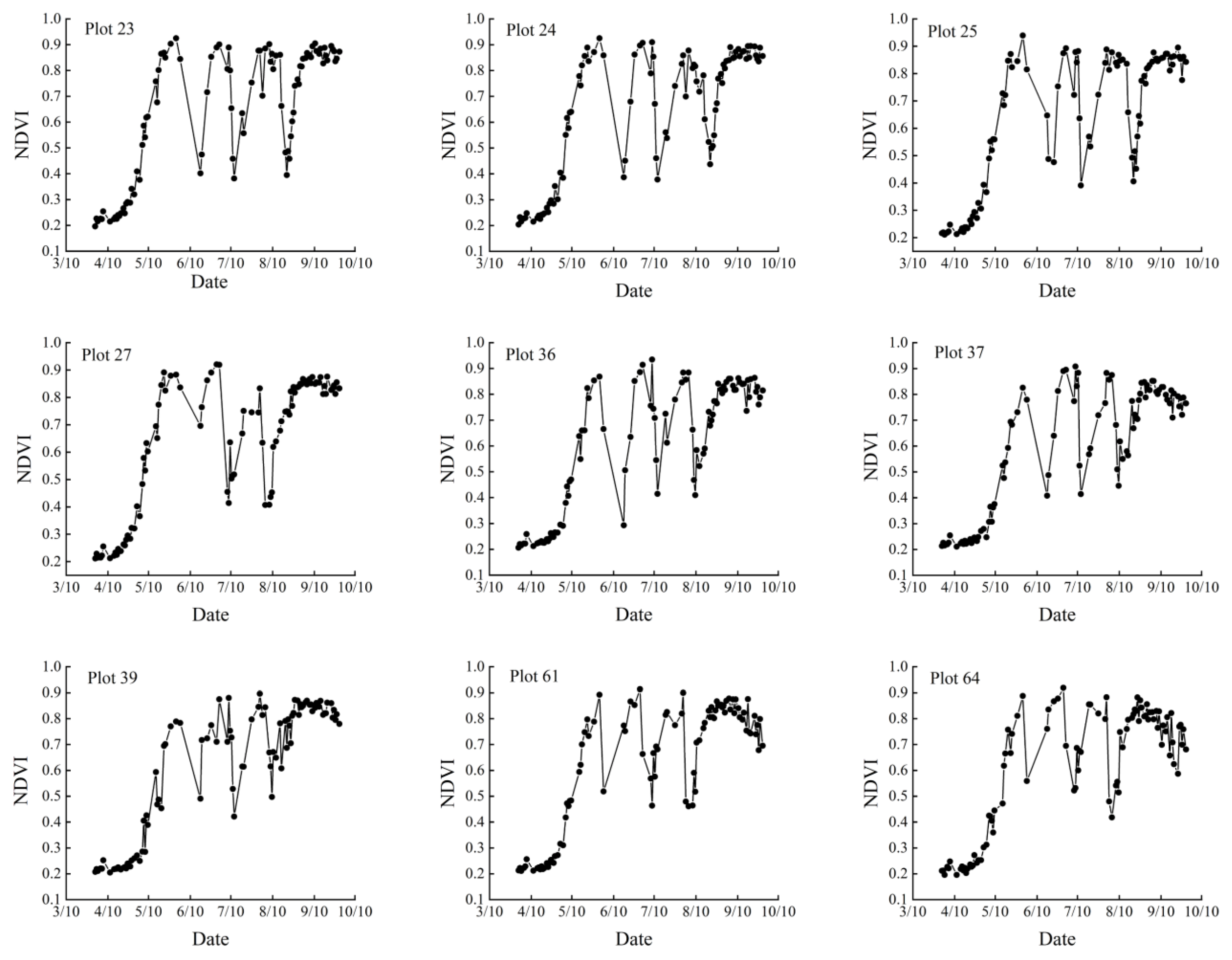
Due to the correlation between the NDVI and vegetation growth status, this study utilized the NDVI to reflect the spatiotemporal variation characteristics of the different alfalfa sampling plots. Based on MODIS MOD09GQ 250 m surface reflectance, the NDVI values of the different alfalfa sampling points from April to September 2022 were calculated, and the results are shown in Figure 2. The alfalfa began to leaf out and started to grow in April, and the NDVI values of the different alfalfa sampling points continued to increase over time. From June to August, the NDVI values suddenly decreased in the different alfalfa sampling plots due to the alfalfa being cut. Different alfalfa sampling plots experienced three wave troughs, indicating a total of three alfalfa harvests. After each alfalfa harvest, the NDVI value gradually increased due to the regenerative characteristics of alfalfa.

3.1.3. Spatial Variation Characteristics of Alfalfa AGB in Different Sampling Plots

The alfalfa spatial variation characteristics were analyzed using NDVI data sourced from Sentinel-2 20 m multispectral data. To maintain the pure pixels involved in the analysis, the analysis range was narrowed inward. The first alfalfa was harvested from the end of May to early June 2022, and the image from 3 June was selected for this study. Overall, there were significant differences in spatial distribution among different alfalfa sampling plots. Compared to other plots, plots 61 and 64 had lower NDVI values due to earlier harvesting; there were also significant differences among other unharvested plots, such as plot 39. Even within the same sampling plot, there were significant spatial differences, such as with plots 36, 37, and 39. The second alfalfa was harvested from the end of June to early July 2022, and the 8 July image was selected for this study. Plots 27, 61, and 64 were harvested earlier than the other plots, with lower NDVI values. The growth of other alfalfa sampling plots was relatively uniform, and the line graph shows that the NDVI values tended to overlap between different alfalfa sampling plots. The third alfalfa harvest was from the end of July to early August, and the 2 August image was selected for this study. Plots 61 and 64 were harvested earlier, with lower NDVI values. The NDVI spatial differences in the alfalfa sampling plots were lower than that of the first-harvest time and larger than that of the second-harvest time (Figure 3).

3.2. Correlation between Different Remote Sensing Indices and Alfalfa Forage Yield/AGB

In 2022, a total of 314 alfalfa field survey samples were collected, and 278 alfalfa sampling points were ultimately selected, with factors such as image date, sampling date matching, and cloud interference considered. This section analyzes the correlations among different band reflectances, vegetation indices, and alfalfa forage yield/AGB, which were obtained from Sentinel-2 MSI images.

3.2.1. Correlation between Different Band Reflectances and Alfalfa Forage Yield/AGB

The correlations among different band reflectances and alfalfa forage yield/AGB are shown in Figure 4. Considering all the alfalfa forage yield/AGB data, the correlation coefficients between different band reflectances and the alfalfa fresh weight were basically above 0.60, and higher correlation coefficients were found in B07 (RE3, central wavelength 783 nm) and B8A (NIR, central wavelength 865 nm), with correlation coefficients above 0.80. The correlations among different band reflectances and alfalfa dry weight were lower than those of fresh weight overall, among which the correlation coefficients were higher in B03 (green, central wavelength 560 nm), B05 (RE1, central wavelength 705 nm), B07 and B8A, with correlation coefficients above 0.70. Overall, based on the alfalfa forage yield data for the three harvest times, the correlations among different band reflectances and the first-harvest alfalfa forage yield were higher than those of the second- and third-harvest times, and the yield of the second-harvest time was higher than that of the third-harvest time.

3.2.2. Correlation between Different Vegetation Indices and Alfalfa Forage Yield/AGB

The correlations among the different vegetation indices and the alfalfa forage yield/AGB are shown in Figure 5. From all alfalfa forage yield/AGB data, the correlation coefficients between the different vegetation indices and the alfalfa fresh weight were basically above 0.70, including the EVI, GNDVI, GVMI, MSAVI, NDII, NDPI, and SAVI. The correlations among different vegetation indices and alfalfa dry weight were lower than those of fresh weight, among which the EVI, GNDVI, GVMI, MSAVI, and NDII had higher correlation coefficients, with values above 0.65. Overall, based on the alfalfa forage yield data from the three harvests, the correlations among different vegetation indices and the first-harvest alfalfa forage yield were higher than those of the second and third harvests.

3.2.3. Regression Analysis of Different Vegetation Indices and Alfalfa Forage Yield/AGB

The results of the regression analysis between the vegetation indices and the alfalfa forage yield/AGB are shown in Figures S1 and S2. From the alfalfa forage yield (fresh weight) data harvested at different times, the correlation between the different vegetation indices and the first-harvest alfalfa forage yield (fresh weight) was better than that of the second- and third-harvest times, the R² values were above 0.50, and the NDWI had the best correlation, with an R² value of 0.60. The correlation between different vegetation indices and the second-harvest alfalfa forage yield (fresh weight) was best with the EVI, with an R² value of 0.33. The correlation coefficients for the other vegetation indices were all less than 0.15, indicating a poor overall correlation. The R² values between different vegetation indices and the third-harvest alfalfa forage yield (fresh weight) were all low, and the correlation was poor. From the alfalfa AGB (fresh weight) data between different harvest times, the correlation between the first and second harvest times was better than that between the second and third harvest times. The best correlation between the first and second harvest times was the EVI, with an R² value of 0.52. The correlation between the second and third harvest times was poor, with R² values less than 0.20. From the total alfalfa forage yield/AGB (fresh weight) data, the GNDVI, NDII, and NDWI had better correlations, with R² values above 0.70. The alfalfa dry weight was similar to the fresh weight, but the R² values of the dry weight were generally lower than those of the fresh weight.

3.3. Alfalfa Forage Yield Inversion Model

3.3.1. Alfalfa Forage Yield Inversion Model Based on a Single Parameter

According to previous analysis, the vegetation indices related to water content had relatively excellent correlations with alfalfa forage yield, such as the GVMI, NDWI, and NDII. Taking the alfalfa forage yield fresh weight as an example, the NDWI was selected as the input variable of the single parameter inversion model, and the alfalfa forage yield inversion models were constructed by different harvest times, including the Exp, LR, RF, SVM and ANN (

Table 3. Alfalfa forage yield inversion model based on a single parameter.

	First-Harvest Time			Second-Harvest Time			Third-Harvest Time
Model	R2	RMSE (g/m2)	Bias (g/m2)	R2	RMSE (g/m2)	Bias (g/m2)	R2	RMSE (g/m2)	Bias (g/m2)
Exp	0.60	338.67	−113.92	0.16	392.74	−146.75	0.16	273.70	186.40
LR	0.55	441.74	−223.04	0.15	413.16	−284.83	0.15	289.90	239.20
RF	0.60	328.11	−60.00	0.07	413.32	−127.80	0.13	330.88	103.65
SVM	0.61	341.99	−137.90	0.15	452.72	−145.90	0.16	259.98	4.34
ANN	0.59	373.64	−155.24	0.15	392.21	−195.20	0.16	388.80	−194.17

). The R² values of the alfalfa forage yield inversion model at the first harvest time were all above 0.55, and the best inversion results were obtained by the Exp, SVM, and RF. The R², RMSE, and bias based on Exp were 0.60, 338.67 g/m² and −113.92 g/m², respectively. The R², RMSE, and bias based on SVM were 0.61, 341.99 g/m², and −137.90 g/m², respectively. The R², RMSE, and bias based on RF were 0.60, 328.11 g/m², and −60.00 g/m², respectively. The accuracy of the alfalfa forage yield inversion model for the second- and third-harvest times was relatively low, with R² values less than 0.20.

3.3.2. Alfalfa Forage Yield Inversion Model Based on Multiple Parameters

This study took the alfalfa fresh weight as a study subject. The band reflectance and vegetation indices were selected based on the correlations among different band reflectances, vegetation indices, and alfalfa forage yield/AGB, for which the correlation coefficient values were above 0.70 (

Table 4. Input variables of the alfalfa forage yield inversion model based on multiple parameters.

	Input Variables
Variable name	NDWI	GVMI	NDII	NDVIRE	MSAVI	NDPI	B07
Correlation coefficient	−0.79	0.78	0.76	0.77	0.75	0.74	0.8

). The multiple-parameter inversion model for alfalfa forage yield was constructed using the selected 8 parameters, including SLR, PLSR, RF, SVM, and ANN.

The inversion effects of alfalfa forage yield based on SVM, and RF were generally superior to those of the other models (

Table 5. Alfalfa forage yield inversion model based on multiple parameters.

	First-Harvest Time			Second-Harvest Time			Third-Harvest Time
Model	R2	RMSE (g/m2)	Bias (g/m2)	R2	RMSE (g/m2)	Bias (g/m2)	R2	RMSE (g/m2)	Bias (g/m2)
SLR	0.55	368.52	−32.07	0.12	364.57	−118.73	0.10	250.66	94.74
PLSR	0.58	344.80	−34.13	0.12	366.19	121.04	0.10	252.39	98.27
RF	0.65	332.32	−2.24	0.31	253.21	48.74	0.11	236.75	43.73
SVM	0.65	329.74	−0.47	0.38	249.11	38.31	0.15	230.77	33.11
ANN	0.57	432.81	−214.91	0.06	421.71	−318.36	0.18	235.02	173.24

). The R² values of the alfalfa forage yield inversion model in the first-harvest time were both 0.65, with RMSEs of 329.74 g/m² and 332.32 g/m² and biases of −0.47 g/m² and −2.24 g/m², respectively. The SVM had a relatively good inversion effect on the second-harvest time, with an R² of 0.38, an RMSE of 249.11 g/m², and a bias of 38.31 g/m²; the next was the RF model, with an R² of 0.31, an RMSE of 253.21 g/m², and a bias of 48.74 g/m². The simulation accuracy of the alfalfa forage yield inversion model for the third-harvest was relatively low, with R² values less than 0.20.

3.3.3. Accuracy Evaluation of the Annual Alfalfa Forage Yield Inversion Model

The annual alfalfa forage yield is composed of the sum of multiple single harvested yields. The study area can be harvested three times a year. This study took the alfalfa forage yield (fresh weight) as the research object, and the validation data of three harvested forage yields were used to evaluate the overall simulation accuracy of the alfalfa annual forage yield. In the annual alfalfa forage yield inversion model based on a single parameter, the Exp and SVM models had relatively high simulation accuracy, with R² values of 0.44, RMSE values of 378.46 g/m² and 436.31 g/m², respectively, and biases of −223.41 g/m² and −298.40 g/m², respectively. In the annual alfalfa forage yield inversion model based on multiple parameters, the accuracies of the SVM and RF simulations were relatively high, with R² values of 0.58, RMSE values of 338.52 g/m² and 342.52 g/m², respectively, and biases of −125.20 g/m² and −124.42 g/m², respectively. Overall, the annual alfalfa forage yield inversion model based on multiple parameters was better than that based on a single parameter, while the simulation accuracies of the SVM and RF models were higher than those of the other models (Figure 6).

4. Discussion

This study compared and analyzed remote sensing inversion models of alfalfa forage yield based on single parameters and multiple parameters by collecting alfalfa forage yield/AGB field survey data at different harvest times to select the optimal alfalfa forage yield inversion model. Water is one of the main components of plants. Gederts [39] elaborated on the importance of plant water content for plant research. Catherine et al. [40] also showed that estimating plant water content was crucial for integrating remote sensing into precision agriculture. The water content of the alfalfa plants in the study area was over 80%. There was a high correlation between the dry weight and fresh weight of the alfalfa (Figure 7). Among the 10 vegetation indices, those with high water correlations, such as the NDII, NDWI, and GVMI, had relatively high coefficients of correlation with alfalfa forage yield/AGB. Moreover, the simulation accuracy of the fresh weight inversion model was higher than that of the dry weight inversion model for both the single-parameter and multiparameter alfalfa forage yield inversion models. Based on the above research results, using vegetation indices closely related to plant water content to establish an inversion model for alfalfa forage yield is a potential approach.

The alfalfa forage yield inversion model for the first-harvest had a good simulation effect at the different harvest times, which may have been due to the differences in alfalfa overwintering ability, which led to significant differences in the growth of the different alfalfa sampling plots. The distribution range of vegetation index values was relatively large, making it suitable for establishing an alfalfa forage yield inversion model. In the later stage, the growth of the second- and third-harvest alfalfa was relatively uniform due to the intervention of manual management measures, and the distribution range of vegetation index values was relatively small and tended to be saturated. Therefore, the simulation accuracy of the alfalfa forage yield inversion model for the second- and third harvests was relatively low. The problem of vegetation index saturation directly affects the accuracy of remote sensing estimations of vegetation parameters [41,42,43]. Chen et al. [44] analyzed the relationship between AGB and band reflectance using partial least squares, combined with the band depth ratio, to improve the estimation method of AGB of high-canopy grasses. The study by Mutanga and Skidmore showed that at high canopy density, pasture biomass may be more accurately estimated by vegetation indices based on wavelengths located in the red edge compared to the standard NDVI [45]. When constructing an inversion model for alfalfa forage yield in this study, the distribution range of vegetation index values was increased by adding alfalfa AGB data between different harvest times, resulting in a higher simulation accuracy of the inversion model. Alfalfa forage yield inversion models based on statistical models and ML were compared in this study. In the alfalfa forage yield inversion model based on a single parameter, the difference in simulation accuracy between the Exp, RF and SVM inversion models was relatively small, and the statistical models could be used when there was only a single parameter to construct an alfalfa forage yield inversion model. The simulation accuracy of the alfalfa forage yield inversion model based on a single parameter was generally lower than that based on multiple parameters, and the simulation accuracy of the RF and SVM models was higher than that of the other alfalfa forage yield inversion models based on multiple parameters. Although the R² in the ANN inversion model performed well, the RMSE and bias were relatively large, which may be due to the small sample size and unsatisfactory model training results.

The study by Tedesco et al. showed that most studies on alfalfa yield estimation focused on biomass estimation [46]. In this study, we utilized the yield/AGB data at different times to construct an alfalfa forage yield inversion model using remote sensing technology, which can estimate year-round alfalfa forage yield rather than instantaneous AGB and is more suitable for actual production. Due to the alfalfa growth characteristics and management measures, the growth of a certain harvest may be relatively uniform, and there may be a saturation phenomenon of the vegetation index in constructing the inversion model, for which the accuracy is not high enough. In this study, we added low AGB data to expand the range of the vegetation index distribution to improve the accuracy of the inversion model, and this method is more suitable for estimating forage yields that are harvested multiple times a year.

5. Conclusions

This study focused on inverse algorithms for alfalfa forage yield in large-scale alfalfa production. The correlations between the reflectance of different satellite remote sensing bands, vegetation indices, and alfalfa forage yield/AGB were analyzed, the suitable bands and vegetation indices for alfalfa forage yield inversion algorithms were screened, and the performances of statistical models and ML algorithms in alfalfa forage yield inversion were comparatively analyzed. The research results indicated that (1) in the alfalfa forage yield inversion model at different harvest times, the first-harvest alfalfa had relatively large differences in growth, and the simulation accuracy of the alfalfa forage yield inversion model was higher than that of the other harvest times. The growth of the second- and third-harvest alfalfa was more homogeneous, and the simulation accuracy of the forage yield inversion model was relatively low. (2) In the alfalfa forage yield inversion model based on a single parameter, the moisture-related vegetation indices had higher coefficients of correlation with alfalfa forage yield/AGB. (3) In the alfalfa forage yield inversion model constructed with vegetation indices and band reflectance as the multiparameter variables, the RF and SVM simulation accuracy was higher than that of the alfalfa forage yield inversion model based on a single parameter. The results of this study can provide technical support for the effective and strategic production management of large-scale alfalfa.

References

- Testa, G.; Gresta, F.; Cosentino, S.L. Dry matter and qualitative characteristics of alfalfa as affected by harvest times and soil water content. Eur. J. Agron. 2011, 34, 144–152. [Google Scholar] [CrossRef]
- Jia, X.; Zhang, Z.; Wang, Y. Forage yield, canopy characteristics, and radiation interception of ten alfalfa varieties in an arid environment. Plants 2022, 11, 1112. [Google Scholar] [CrossRef]
- Arshad, M.; Feyissa, B.A.; Amyot, L.; Aung, B.; Hannoufa, A. MicroRNA156 improves drought stress tolerance in alfalfa (Medicago sativa) by silencing SPL13. Plant Sci. 2017, 258, 122–136. [Google Scholar] [CrossRef]
- Lei, Y.; Hannoufa, A.; Yu, P. The use of gene modification and advanced molecular structure analyses towards improving alfalfa forage. Int. J. Mol. Sci. 2017, 18, 298. [Google Scholar] [CrossRef]
- Wang, Q.; Zou, Y. China’s alfalfa market and imports: Development, trends, and potential impacts of the U.S.–China trade dispute and retaliations. J. Integr. Agric. 2020, 19, 1149–1158. [Google Scholar] [CrossRef]
- Bai, Z.; Lee, M.R.F.; Ma, L.; Ledgard, S.; Oenema, O.; Velthof, G.L.; Ma, W.; Guo, M.; Zhao, Z.; Wei, S.; et al. Global environmental costs of China’s thirst for milk. Glob. Chang. Biol. 2018, 24, 2198–2211. [Google Scholar] [CrossRef]
- Wang, Y.; Zhao, Y.; Xue, F.; Nan, X.; Wang, H.; Hua, D.; Liu, J.; Yang, L.; Jiang, L.; Xiong, B. Nutritional value, bioactivity, and application potential of Jerusalem artichoke (Helianthus tuberosus L.) as a neotype feed resource. Anim. Nutr. 2020, 6, 429–437. [Google Scholar] [CrossRef]
- Liu, M.; Yang, M.; Yang, H. Biomass production and nutritional characteristics of quinoa subjected to cutting and sowing date in the midwestern China. Grassl. Sci. 2020, 67, n215–n224. [Google Scholar] [CrossRef]
- Feng, L.; Zhang, Z.; Ma, Y.; Du, Q.; Williams, P.; Drewry, J.; Luck, B. Alfalfa yield prediction using uav-based hyperspectral imagery and ensemble learning. Remote Sens. 2020, 12, 2028. [Google Scholar] [CrossRef]
- Noland, R.L.; Wells, M.S.; Coulter, J.A.; Tiede, T.; Baker, J.M.; Martinson, K.L.; Sheaffer, C.C. Estimating alfalfa yield and nutritive value using remote sensing and air temperature. Field Crops Res. 2018, 222, 189–196. [Google Scholar] [CrossRef]
- Wang, R.; Shi, F.; Xu, D. The extraction method of alfalfa (Medicago sativa L.) mapping using different remote sensing data sources based on vegetation growth properties. Land 2022, 11, 1996. [Google Scholar] [CrossRef]
- Mulianga, B.; Bégué, A.; Simoes, M.; Todoroff, P. Forecasting regional sugarcane yield based on time integral and spatial aggregation of MODIS NDVI. Remote Sens. 2013, 5, 2184–2199. [Google Scholar] [CrossRef]
- Cai, Y.; Guan, K.; Peng, J.; Wang, S.; Seifert, C.; Wardlow, B.; Li, Z. A high-performance and in-season classification system of field-level crop types using time-series Landsat data and a machine learning approach. Remote Sens. Environ. 2018, 210, 35–47. [Google Scholar] [CrossRef]
- Xie, Y.; Sha, Z.; Yu, M. Remote sensing imagery in vegetation mapping: A review. J. Plant Ecol. 2008, 1, 9–23. [Google Scholar] [CrossRef]
- Jin, X.; Kumar, L.; Li, Z.; Feng, H.; Xu, X.; Yang, G.; Wang, J. A review of data assimilation of remote sensing and crop models. Eur. J. Agron. 2018, 92, 141–152. [Google Scholar] [CrossRef]
- Wang, X.; Yu, S.; Wen, Z.; Zhang, L.; Fang, C.; Jiang, L. Application of modern GIS and remote sensing technology based on big data analysis in intelligent agriculture. J. Indian Soc. Remote Sens. 2022, 1–11. [Google Scholar] [CrossRef]
- Atzberger, C. Advances in remote sensing of agriculture: Context description, existing operational monitoring systems and major information needs. Remote Sens. 2013, 5, 949–981. [Google Scholar] [CrossRef]
- Meroni, M.; Marinho, E.; Sghaier, N.; Verstrate, M.M.; Leo, O. Remote sensing based yield estimation in a stochastic framework—Case study of durum wheat in Tunisia. Remote Sens. 2013, 5, 539–557. [Google Scholar] [CrossRef]
- Mahlayeye, M.; Darvishzadeh, R.; Nelson, A. Cropping patterns of annual crops: A remote sensing review. Remote Sens. 2022, 14, 2404. [Google Scholar] [CrossRef]
- Kamble, B.; Irmak, A.; Hubbard, K.; Gowda, P. Irrigation scheduling using remote sensing data assimilation approach. Adv. Remote Sens. 2013, 02, 258–268. [Google Scholar] [CrossRef]
- Bolton, D.K.; Friedl, M.A. Forecasting crop yield using remotely sensed vegetation indices and crop phenology metrics. Agric. For. Meteorol. 2013, 173, 74–84. [Google Scholar] [CrossRef]
- Islam, M.D.; Di, L.; Qamer, F.M.; Shrestha, S.; Guo, L.; Lin, L.; Mayer, T.J.; Phalke, A.R. Rapid rice yield estimation using integrated remote sensing and meteorological data and machine learning. Remote Sens. 2023, 15, 2374. [Google Scholar] [CrossRef]
- Fan, X.; He, G.; Zhang, W.; Long, T.; Zhang, X.; Wang, G.; Sun, G.; Zhou, H.; Shang, Z.; Tian, D.; et al. Sentinel-2 images based modeling of grassland above-ground biomass using random forest algorithm: A case study on the Tibetan Plateau. Remote Sens. 2022, 12, 5321. [Google Scholar] [CrossRef]
- Bognár, P.; Ferencz, C.S.; Pásztor, S.; Molnár, G.; Timár, G.; Hamar, D.; Lichtenberger, J.; Székely, B.; Steinbach, P.; Ferencz, O.E. Yield forecasting for wheat and corn in Hungary by satellite remote sensing. Int. J. Remote Sens. 2011, 32, 4759–4767. [Google Scholar] [CrossRef]
- Weiss, M.; Jacob, F.; Duveiller, G. Remote sensing for agricultural applications: A meta-review. Remote Sens. Environ. 2020, 236, 111402. [Google Scholar] [CrossRef]
- Kayad, A.G.; Al-Gaadi, K.A.; Tola, E.; Madugundu, R.; Zeyada, A.M.; Kalaitzidis, C. Assessing the spatial variability of alfalfa yield using satellite imagery and ground-based data. PLoS ONE 2016, 11, e0157166. [Google Scholar] [CrossRef]
- Azadbakht, M.; Ashourloo, D.; Aghighi, H.; Homayouni, S.; Hahrabi, H.S.; Matkan, A.; Radiom, S. Alfalfa yield estimation based on time series of Landsat 8 and PROBA-V images: An investigation of machine learning techniques and spectral-temporal features. Remote Sens. Appl. Soc. Environ. 2022, 25, 2352–9385. [Google Scholar] [CrossRef]
- Zhou, Y.; Colton Flynn, K.; Gowda, H.P.; Wagle, P.; Ma, S.; Kakani, G.V.; Jean, L.; Steiner, J.L. The potential of active and passive remote sensing to detect frequent harvesting of alfalfa. Int. J. Appl. Earth Obs. Geoinf. 2021, 104, 102539. [Google Scholar] [CrossRef]
- Liao, L.; Song, J.; Wang, J.; Xiao, Z.; Wang, J. Bayesian method for building frequent Landsat-like NDVI datasets by integrating MODIS and Landsat NDVI. Remote Sens. 2016, 8, 452. [Google Scholar] [CrossRef]
- Huete, A.J.C.; Liu, H. Development of vegetation and soil indices for MODIS-EOS. Remote Sens. Environ. 1994, 49, 224–234. [Google Scholar] [CrossRef]
- McFeeters, S.K. The use of the Normalized Difference Water Index (NDWI) in the delineation of open water features. Int. J. Remote Sens. 2007, 17, 1425–1432. [Google Scholar] [CrossRef]
- Xu, D.; Wang, C.; Chen, J.; Shen, M.; Shen, B.; Yan, R.; Li, Z.; Karnieli, A.; Chen, J.; Yan, Y.; et al. The superiority of the normalized difference phenology index (NDPI) for estimating grassland aboveground fresh biomass. Remote Sens. Environ. 2021, 264, 112578. [Google Scholar] [CrossRef]
- Huete, A.R. A soil-adjusted vegetation index (SAVI). Remote Sens. Environ. 1988, 25, 295–309. [Google Scholar] [CrossRef]
- Guo, S.; Ruan, B.; Chen, H.; Guan, X.; Wang, S.; Xu, N.; Li, Y. Characterizing the spatiotemporal evolution of soil salinization in Hetao Irrigation District (China) using a remote sensing approach. Int. J. Remote Sens. 2018, 39, 6805–6825. [Google Scholar] [CrossRef]
- Sow, M.; Mbow, C.; Hély, C.; Fensholt, R.; Sambou, B. Estimation of herbaceous fuel moisture content using vegetation indices and land surface temperature from MODIS data. Remote Sens. 2013, 5, 2617–2638. [Google Scholar] [CrossRef]
- Ceccato, P.; Gobron, N.; Flasse, S.; Pinty, B.; Tarantola, S. Designing a spectral index to estimate vegetation water content from remote sensing data: Part 1Theoretical approach. Remote Sens. Environ. 2002, 82, 188–197. [Google Scholar] [CrossRef]
- Ettehadi Osgouei, P.; Kaya, S.; Sertel, E.; Alganci, U. Separating built-up areas from bare land in mediterranean cities using Sentinel-2A imagery. Remote Sens. 2019, 11, 345. [Google Scholar] [CrossRef]
- Gitelson, A.; Merzlyak, M.N. Spectral reflectance changes associated with autumn senescence of Aesculus hippocastanum L. and Acer platanoides L. Leaves. spectral features and relation to Chlorophyll estimation. J. Plant Physiol. 1994, 143, 286–292. [Google Scholar] [CrossRef]
- Ievinsh, G. Water Content of Plant Tissues: So Simple That Almost Forgotten? Plants 2023, 12, 1238. [Google Scholar] [CrossRef]
- Catherine, M.; Karl, S.; Abdou, B.; Heather, M.; Jean-Claude, D. Validation of a hyperspectral curve-correlationting model for the estimation of plant water content of agricultural canopies. Remote Sens. Environ. 2003, 87, 148–160. [Google Scholar] [CrossRef]
- Aklilu Tesfaye, A.; Gessesse Awoke, B. Evaluation of the saturation property of vegetation indices derived from sentinel-2 in mixed crop-forest ecosystem. Spat. Inf. Res. 2021, 29, 109–121. [Google Scholar] [CrossRef]
- Todd, S.W.; Hoffer, R.M.; Milchunas, D.G. Biomass estimation on grazed and ungrazed rangelands using spectral indices. Int. J. Remote Sens. 1988, 19, 427–438. [Google Scholar] [CrossRef]
- Thenkabail, P.S.; Smith, R.B.; De Pauw, E. Hyperspectral vegetation indices and their relationships with agricultural crop characteristics. Remote Sens. Environ. 2000, 71, 158–182. [Google Scholar] [CrossRef]
- Chen, J.; Gu, S.; Shen, M.; Tang, Y.; Matsushita, B. Estimating aboveground biomass of grassland having a high canopy cover: An exploratory analysis of in situ hyperspectral data. Int. J. Remote Sens. 2009, 30, 6497–6517. [Google Scholar] [CrossRef]
- Mutanga, O.; Skidmore, A.K. Narrow band vegetation indices overcome the saturation problem in biomass estimation. Int. J. Remote Sens. 2004, 25, 3999–4014. [Google Scholar] [CrossRef]
- Tedesco, D.; Nieto, L.; Hernández, C.; Rybecky, J.F.; Min, D.; Sharda, A.; Hamilton, K.J.; Ciampitti, I.A. Remote sensing on alfalfa as an approach to optimize production outcomes: A review of evidence and directions for future assessments. Remote Sens. 2022, 14, 4940. [Google Scholar] [CrossRef]
Figure 1.
Location of the study area and field sampling points.
Figure 2.
The alfalfa temporal variation characteristics in different sampling plots.