Assessment of the Spatial Variability and Uncertainty of Shreddable Pruning Biomass in an Olive Grove Based on Canopy Volume and Tree Projected Area

Abstract

Olive pruning residues are a by-product that can be applied to soil or used for energy production in a circular economy model. Its benefits depend on the amount of pruning, which varies greatly within farms. This study aimed to investigate the spatial variability of shreddable olive pruning in a traditional olive grove in Córdoba (Spain) with an area of 15 ha and trees distanced 12.5 m from each other. To model the spatial variability of shreddable olive pruning, geostatistical methods of stochastic simulation were applied to three correlated variables measured on sampled trees: the crown projected area (n = 928 trees), the crown volume (n = 167) and the amount of shreddable pruning (n = 59). Pearson’s correlation between pairs of variables varied from 0.71 to 0.76. The amount of pruning showed great variability, ranging from 7.6 to 76 kg tree⁻¹, with a mean value of 37 kg tree⁻¹. Using exponential and spherical variogram models, the spatial continuity of the variables under study was established. Shreddable dry pruning weight values showed spatial autocorrelation up to 180 m. The spatial uncertainty of the estimation was obtained using sequential simulation algorithms. Stochastic simulation algorithms provided 150 possible images of the amount of shreddable pruning on the farm, using tree projected area and crown volume as secondary information. The interquartile range and 90% prediction interval were used as indicators of the uncertainty around the mean value. Uncertainty validation was performed using accuracy plots and the associated G-statistic. Results indicate with high confidence (i.e., low uncertainty) that shreddable dry pruning weight in the mid-western area of the farm will be much lower than the rest of the farm. In the same way, results show with high confidence that dry pruning weight will be much higher in a small area in the middle east of the farm. The values of the G-statistic ranged between 0.89 and 0.90 in the tests performed. The joint use of crown volume and projected areas is valuable in estimating the spatial variability of the amount of pruning. The study shows that the use of prediction intervals enables the evaluation of farm areas and informed management decisions with a low level of risk. The methodology proposed in this work can be extrapolated to other 3D crops without requiring modifications. On a larger scale, it can be useful for predicting optimal locations for biomass plants, areas with high potential as carbon sinks or areas requiring special soil protection measures.

1. Introduction

Olive trees, widely cultivated across the globe, cover a vast surface area that exceeds 10 Mha [1]. Olive groves in the Mediterranean basin are particularly relevant, accounting for approximately 95% of the total global cultivation area and contributing to over 85% of the world’s olive oil production [1]. In Spain, the primary olive-producing country, olives are the most important crop, occupying more than 2.7 Mha and yielding a production surpassing 6 Mt [2]. With the exception of Cantabria and Asturias, which have cool and rainy summers, olive production occurs in all Spanish regions [3].

Although native to the Mediterranean region, the olive tree is a crop with broad adaptability. Generally, the olive tree has modest soil requirements and can thrive in a wide range of soils, many of which are marginal for other crops [4]. Currently, olive trees are cultivated in all regions of the globe between 30° and 45° latitude in both hemispheres, from desert areas to more humid climates [5]. They tolerate slightly acidic soils (pH levels above 6) as well as alkaline soils. However, very acidic or highly alkaline soils can adversely affect nutrient availability and tree health. Well-drained and moderately fertile soils are recommended [4].

Tillage is the most common soil management practice in olive groves, particularly in Mediterranean Europe [6]. In this system, the soil is kept bare of vegetation for most of the year through tillage. Various implements are used for this purpose, such as cultivators, vibrocultivators (a type of cultivator that utilizes vibration for soil preparation) and spiked harrows [7]. The depth of tillage has decreased over time due to higher production costs and a growing awareness of the negative impacts of excessive soil disturbance. Until the second half of the last century, tillage did not represent a serious threat to olive orchard sustainability since the extent of agricultural mechanization was limited. However, the widespread use of tractors and new, more powerful agricultural machinery, coupled with tillage intensification, has resulted in soil degradation [7].

Olive groves, often cultivated on steep slopes, are prone to severe water erosion due to unprotected soils and intense rainfall. These erosive processes lead to significant soil loss [8], causing damage to both on-farm and off-farm areas [9]. Despite the recent expansion of olive tree cultivation in flatter terrains, erosion continues to pose a significant challenge in olive groves. Notably, a substantial portion of agricultural land in Spain, approximately 13%, is confronted with the imminent threat of severe or very severe erosion [10].

The Mediterranean climate is characterized by xeric humidity [11]. It does not favor the maintenance of a persistent vegetation canopy, particularly following the prolonged and sweltering summer season, during which natural wildfires are frequent. This climate experiences a cold and wet period during the autumn and winter months, which accounts for approximately 80% of the total annual precipitation, followed by a very arid and hot period in the spring and summer.

A practical solution against soil loss is the establishment of sown groundcovers or spontaneous vegetation, with low implantation costs. They provide valuable ecosystem services [12]. However, they compete for water with the crop and are not very durable once killed by mowing or herbicides [13,14].

The mulching of shreddable pruning residues is a very good alternative to protecting the soil while simultaneously improving its physical, chemical and biological properties [15,16,17]. Pruning mulch is effective in soil and water conservation [18,19], and provides longer protection than herbaceous groundcovers [20]. Chopping the residues improves soil fertility [21], partially prevents the development of ruderal flora [22], may reduce the use of herbicides, and does not pose a phytopathological problem on any farm with proper phytosanitary status [23].

The utilization of pruning residues generated in olive orchards as organic soil amendment has been demonstrated as an effective approach to enhancing the soil capacity to sequester carbon continuously [24,25], thus contributing to the mitigation of CO₂ emissions [26]. In a six-year experiment, Nieto et al. [26] observed a carbon increment of 0.5 t C ha⁻¹ yr⁻¹, which is consistent with the findings reported by Mairech et al. [24].

The establishment of pruning mulch, or a concomitant application of pruning mulch and spontaneous grasses, exerts a significant impact on predator and parasitoid species linked to distinct olive pests. This combination has been documented to stimulate the heterogeneity and richness of advantageous arthropods, which play a pivotal role in the domain of biological pest management [27].

The use of chopped pruning residues by farmers has been increasing [28]. According to the recent “Law 7/2022, of April 8, on waste and contaminated soils for a circular economy” [29], these residues cannot be burned, except for authorized exceptions. Likewise, their use as an inert cover is one of the objectives of the Common Agricultural Policy 2023–2027, which has recently come into effect (Official State Bulletin, number 308, 24/12/22, Spain). Therefore, an increase in the area of olive groves managed with pruning mulch is expected.

The source of this cover is the pruning of the crop, generally performed annually or biannually. Significant amounts of ligneous biomass can be obtained from the pruning operations, ranging between 1.3 and 3.0 t ha⁻¹ yr⁻¹ [30]. This biomass is typically piled and burned on the farm, either to reduce the hazard of accidental fires or to prevent the transmission of diseases and pests. This implies a significant workload and a source of CO₂ emission. Alternatively, pruning residues can be used as biomass or in biorefineries as an energy source, although their potential use is largely limited by the spatial extent of agricultural activities, temporal supply fluctuations and technical difficulties, such as collecting and processing [31].

The potential of chopped mulch, either to improve soil properties [32] or for use as biomass, will depend on the available amount of pruning. The quantity of pruning biomass is strongly linked to the size of the olive trees [19], resulting in varying densities of mulch in fields with trees of different sizes. Accurate knowledge of the amount of shreddable pruning is crucial for efficient farm management. However, direct measurement of pruning biomass through in situ weighing is prohibitively expensive. Hence, it is important to explore the use of auxiliary variables that can aid in estimation and are easily obtainable through field sampling or image analysis [33].

In this sense, crown volume and projected area of the olive trees are found to be correlated [34], and a linear relationship between crown volume and shreddable pruning weight has been reported [19]. There are several methods to obtain tree crown volumes. Its conventional estimation can be accomplished by field work—the only option available to the farmer [35]. Allometric equations can be used to calculate crown volume or even pruning quantities based on dendrometric parameters, although there is some discussion about their application to fruit trees [36]. In general, the use of proximal multiparametric sensors [37], LiDAR, or terrestrial laser scanning [38] can facilitate the estimation of available biomass through rapid, nondestructive methods. Additionally, geographic information system software can serve as a valuable tool for managing and analyzing geographic data related to the localization of pruning residues, particularly in the planning of the energy supply chain [39].

In a more detailed analysis, LiDAR can be classified into ground-based, airborne and satellite systems. The first group includes terrestrial laser scanners and mobile terrestrial laser scanners (MTLS), which are commonly applied in agriculture [38]. However, they have limitations when it comes to large plots, such as the one presented in this study [40]. Furthermore, they are expensive, requiring several scanning stations to ensure complete coverage of tree surfaces, which can be time-consuming [41]. Additionally, substantial computing resources are needed to handle the large datasets. Limitations have also been reported for MTLS systems mounted on moving vehicles in terms of data registration inside tree crowns [42]. Airborne LiDAR systems enable the registration of all trees within a plot, including those planted very close together, which can be challenging to measure using other LiDAR techniques. Nevertheless, there are drawbacks associated with aircraft-based systems, such as limited data acquisition from the lower parts of the canopy.

Unmanned Aerial Vehicle (UAV) systems equipped with LiDAR sensors offer a cost-effective and efficient solution for collecting data from specific plots. A study conducted by Dalla et al. [43] found good correlations between Terrestrial Laser Scanning and UAV-LiDAR data for stems and branches with diameters exceeding 30 cm. However, it was observed that the accuracy of UAV-LiDAR data was lower for young trees. However, fruit trees typically have thinner stems compared to those found in forested areas. They often exhibit leaning characteristics and irregularities due to growth or pruning, and rarely reach the height at which Diameter at Breast Height (DBH) is typically measured (1.30 m). Although these systems can offer valuable data for extracting tree and height models, additional analysis is necessary to precisely determine trunks and three-dimensional crown structures. Currently, only the 3D points of the outermost parts of the canopies are captured.

Therefore, there are a wide variety of options for the determination of canopy volume and, occasionally, available biomass. However, to the best of our knowledge, there are no published works about methods to estimate the shreddable pruning biomass in crops and its spatial uncertainty using stochastic simulation algorithms. Sequential simulation algorithms can use data obtained from any of the above-mentioned technologies while simultaneously incorporating their spatial information, such as autocorrelation and cross-correlation.

In this sense, to make farm management decisions, it is crucial to have information on the spatial patterns of tree attributes that allow estimating the spatial variation of pruning biomass on a farm. As stated by Cambardella et al. [44] and Rodríguez-Lizana et al. [19], the amount of pruning residue on an agricultural farm exhibits spatial autocorrelation. Beyond estimation, stochastic sequential simulation algorithms, such as Gaussian sequential simulation or direct sequential simulation, can be utilized to quantify and map the spatial uncertainty of predictions (estimations) in unsampled areas [45,46]. Assessing the uncertainty of a variable is usually a preliminary step to evaluating the risk associated with any decision-making process [47].

The current study proposes using tree projected area and crown volume as auxiliary variables to estimate the amount of shreddable pruning biomass per tree in a traditional olive orchard, and specifically aims to: (i) assess the spatial variability of the amount of shreddable pruning per tree, tree projected areas and crown volumes in a traditional olive orchard, (ii) estimate the average amount of shreddable pruning on a farm incorporating the spatial dimension and (iii) determine the spatial uncertainty of this amount through stochastic simulation algorithms conditioned on the available data.

2. Materials and Methods

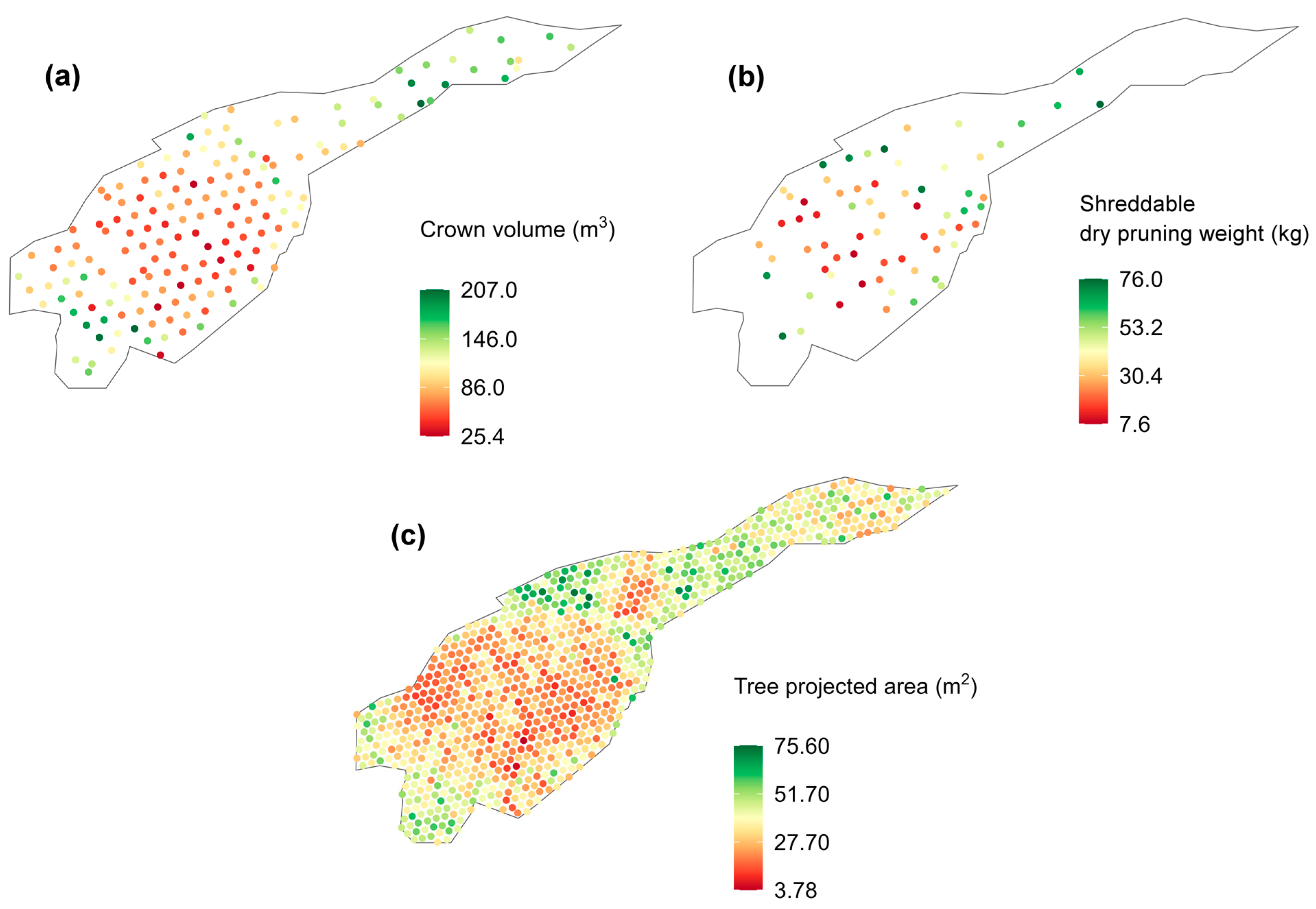
2.1. Study Area and Field Sampling

The research was conducted in a rainfed olive grove located in Fernán-Núñez (Córdoba, Spain) (Figure 1A), with an area of 15 ha and 928 olive trees. Soil corresponds to a Vertic haploxerept according to the Soil Survey Staff’s (2014) classification. The soil textural class is characterized as silty clay. Detailed physical and chemical properties of the soil are presented in

Table 1. Physicochemical characteristics of the soil.

Depth (cm)	pH (H2O)	pH (Cl2Ca)	Sand (%)	Silt (%)	Clay (%)	OC (g kg−1)	CaCO3 (%)	CEC (cmolc kg−1)
0–10	8.2	7.8	6.2	44.7	49.1	7.7	28.6	25
10–20	8.2	7.8	10.3	40.4	49.3	6.8	28.9	22
20–40	8.4	7.8	8.1	42.9	49.0	6.1	30.7	24
40–60	8.5	7.8	8.5	43.0	48.5	5.7	32.5	22

OC: organic carbon; CEC: cation exchange capacity.

.

This soil is very suitable for olive cultivation. It is a soil with a high clay content that is partially expansive, which gives it certain vertic characteristics such as moisture retention, an aspect of interest given the climate of the area. It has a high calcium carbonate content, and the olive trees are well adapted to calcareous soils. The calcium carbonate buffers the pH to values slightly higher than 8, which are ideal for this plant. It has no internal drainage limitations or waterlogging, making it less susceptible to fungal diseases. It does not exhibit textural contrasts, thus making it suitable for this plant [4].

The study area (Figure 1B) is located in a Mediterranean region with a climatic pattern characterized by arid summers accompanied by high temperatures and wet winters. The climate of the area is optimal for the growth of olive trees, as it is inherently adapted to it. The predominant climate in this region corresponds to the Csa classification of the Köppen-Geiger system [48]. Therefore, it has a temperate climate, as denoted by the first letter (C) of the classification. The second letter, “s”, indicates that it has a dry summer, as the precipitation of the driest month in summer is less than 40 mm and less than one-third of the precipitation of the wettest month in winter. Finally, the third letter, “a”, signifies that it has a hot summer, with average monthly temperatures exceeding 22 °C.

Mean annual precipitation is 507 mm. According to the data from AEMET [49], the relative humidity is 60%, with an insolation of 242 h month⁻¹. There are 5 months of frost risk.

Table 2. Monthly minimum, mean and maximum temperature and rainfall in the Santaella weather station. Period: 2000–2022.

	Jan	Feb	Mar	Apr	May	Jun	Jul	Aug	Sep	Oct	Nov	Dec
Rainfall (mm)	49.1	51.8	70.7	51.8	36.0	6.0	0.5	5.0	22.2	64.5	71.7	77.6
	Monthly temperature (°C)
Maximum	14.6	16.4	19.4	22.6	27.4	32.7	36.5	36.2	30.9	25.6	18.4	15.5
Mean	9.2	10.6	13.0	15.8	19.9	24.4	27.5	27.5	23.4	19.0	12.9	10.3
Minimum	4.2	5.1	7.3	9.8	12.8	16.2	18.6	19.2	16.8	13.4	7.9	5.7

shows the monthly average data of precipitation and minimum, mean and maximum temperatures collected from 2000 to the present by the Santaella weather station (37°31′25″ N, 4°53′3″ W; 207 m above sea level) belonging to the “Consejería de Agricultura, Pesca y Desarrollo Rural de Andalucía”.

The plantation pattern is quincunx, with trees distanced 12.5 m from each other. The trees are over 50 years old, and almost all of them have between two and four trunks. This olive plantation well represents the traditional olive groves in the area.

Pruning of the trees on the farm was carried out between 2/2/21 and 12/2/21. Measurements of tree crown volume (Figure 2a) were taken before pruning, between 20/1/21 and 28/1/21. A total of 167 trees were randomly selected, covering the entire study area. The crown volume was determined using the ellipsoid volume method, widely used in isolated trees [19,35]. This method consists of the measurement of three semiaxes of the olive tree, after which the volume is obtained according to Equation (1):

V_E = 4π/3 × E_a × E_b × E_c

(1)

E_a and E_b correspond to the canopy length and width semiaxes, respectively. To obtain the semiaxis E_c, the tree height and the height of the first leaves were measured with a ruler. E_c was calculated as the semidifference between both.

After pruning the plantation, 59 trees were randomly selected (Figure 2b), and their pruning was weighed with the use of a manual scale. Only pruning branches smaller than 8 cm in diameter (shreddable pruning material) were included. Branches greater than 8 cm in diameter were cut with a chainsaw and removed before chopping with agricultural machinery, following the manufacturer’s recommendations. Five samples of the material to be chopped were taken to the laboratory, where they were placed in an oven at 80º until they reached a constant weight in order to determine their moisture content and estimate the dry weight of the samples.

Likewise, the projected areas of all the trees in the plantation were determined by image analysis (Figure 2c), using ImageJ software using a two-phase procedure, as detailed in Rodríguez-Lizana et al. [34].

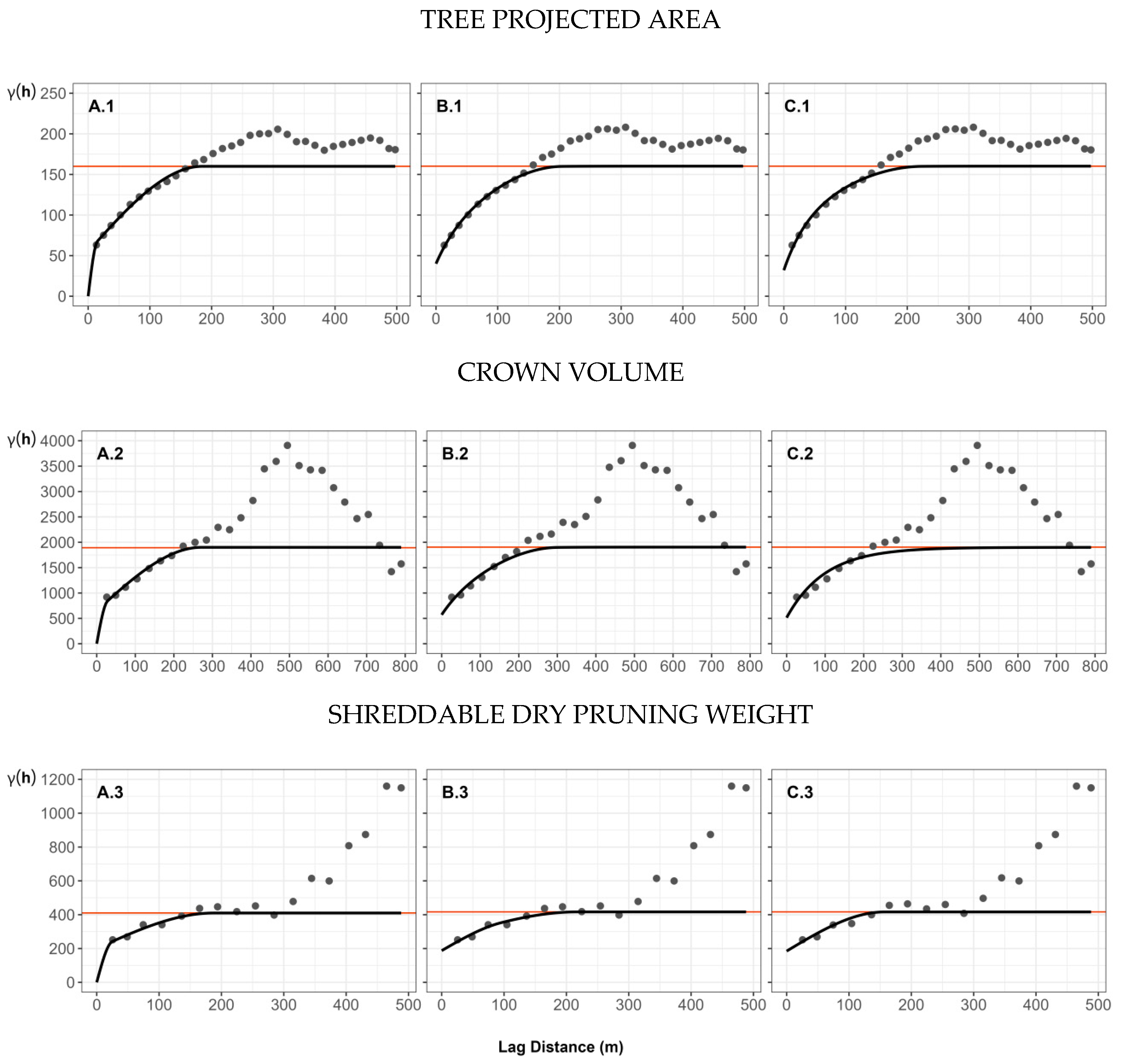
2.2. Geostatistical Analysis

Univariate descriptive statistics and Pearson’s correlation coefficients between pairs of variables were estimated for shreddable dry pruning material, tree projected area and crown volume using field and laboratory data. Geostatistical methods and algorithms were then applied for the analysis and modeling of the spatial correlation of each variable, to estimate their mean values at every location and to assess the impacts of spatial uncertainty on the estimated values. The spatial autocorrelation of variables i, $Z_i$, was quantified with an empirical semivariogram ${\widehat{\gamma }}_{z_i}\left(h\right)$, which was obtained from $n$ data observations $z_i\left(s_{\alpha }\right)$ located at coordinates $s_{\alpha }$ separated by a distance $h$ and represents average dissimilarity values at discrete distance intervals (2).

$${\widehat{\gamma }}_{z_i}\left(h\right)=\frac{1}{2n}{\displaystyle \sum }_{\alpha =1}^n{\left[z_i\left(s_{\alpha }\right)-z_i\left(s_{\alpha }+h\right)\right]}^2$$

(2)

To estimate the spatial autocorrelation for any distance (and not only for discrete distance intervals), semivariogram models belonging to the family of positive definite functions were fitted to their empirical estimates. Widely used in environmental sciences applications are the exponential, Gaussian and spherical functions [50]. In this work, instead of fitting individual semivariogram models, linear combinations of semivariograms (nested models) were considered improving the fit. It is well known that the sum of positive definite functions is also a positive definite function [51], so the inclusion of any linear combination of the above-referred models can be used. The mathematical expression for the nested function with $M$ semivariogram models can be summarized as follows (3):

$${\gamma }_{z_i}\left(h\right)=c_0+{\displaystyle \sum }_{m=1}^M{\gamma }_{z_i, m}\left(h;c_m, a_m\right)$$

(3)

where $c_0$ is a parameter representing the nugget-effect, and ${\gamma }_{z_i, m}\left(h;c_m;a_m\right)$ is the semivariogram model $m$ for variable $Z_i$, which is a function of distance with parameters range ($a_m$), and partial sill ($c_m$). For variable $Z_i$, the semivariogram parameters ($c_0, c_m,a_m$) with $m=1,\dots ,M$, were estimated with a nonlinear weighted least squares estimator. The number and type of nested functions chosen to fit empirical semivariograms are user decisions. Depending on the variable chosen, three different combinations of nested models with spherical and exponential functions were considered appropriate for an accurate fit, reflecting as closely as possible the spatial structure found in the observed data.

To estimate mean values at every location and quantify the spatial uncertainty of the estimated values for shreddable dry pruning material, stochastic simulation algorithms were applied to each variable over a dense simulation grid (1 × 1 m) covering the study area. First, observed (conditioning) data of tree projected area variable and its nested models fitted previously were used with the direct sequential simulation (DSS) algorithm [45] to estimate local mean and variances at every grid node (n = 149,338). Then, a direct sequential cosimulation (coDSS) algorithm was used with a Markov-type approximation [51] to derive crown volume. As input, the algorithm required not only the observed data for crown volume and the nested semivariogram model, but also the collocated values previously simulated for tree projected area and the Pearson’s correlation coefficient between them. In a final step, for shreddable dry pruning material, a similar cosimulation algorithm was applied, but now using the collocated values previously simulated for crown volume and their Pearson’s correlation coefficient.

Once the simulations of dry pruning weight for each of the three nested models were generated, the analysis of different spatial patterns of uncertainty was performed with the visualization of different quantile maps (e.g., 5-th, 25-th, 50-th, 75-th or 95-th quantiles) drawn from simulations. For assessment and selection of the “best”uncertainty results (as they differ in the fitted semivariogram model), the accuracy plot and the associated G-statistic were computed as proposed by Deutsch [52]. The accuracy plot consists of a scatterplot that compares the proportion of times true (observed) values fall into the symmetric p-probability interval, with expected probability p. A diagonal line is drawn to guide the interpretation of results: the closer the points are to the line, the better the uncertainty model is. The computation of G-statistic complements this plot, by quantifying the closeness with the following integral (4):

$$G=1-{{\displaystyle \int }}_0^1\left[3*a\left(p\right)-2\right]\left[\overline{\xi }\left(p\right)-p\right]dp$$

(4)

where $\overline{\xi }\left(p\right)$ is the proportion of observed values falling in the symmetric p-probability interval, and $a\left(p\right)=1$ if $\overline{\xi }\left(p\right)>p$ and 0 otherwise.

2.3. Software

R was employed for descriptive statistical analysis of the variables shreddable dry pruning weight, crown volume and tree projected area. It was also used for variogram calculation, to check the performance of DSS and CoDSS outputs, and to preview and create the maps [53]. ImageJ [54] was employed to determine tree projected areas of the farm. Stochastic simulations were generated with a script written in C++. An R routine was developed to evaluate the goodness of fit of the spatial uncertainty model, as well as to determine descriptive statistics per pixel, interquartile range and 90% prediction interval.

3. Results and Discussion

3.1. Statistics of Field and Laboratory Variables

The variables studied show strong field variability, as evidenced by their coefficients of variation, which range between 0.36 and 0.55 (

Table 3. Descriptive statistics of the field and laboratory variables.

	Mean ± SE	Coefficient of Variation	Minimum	Lower Quartile	Median	Upper Quartile	Maximum
Shreddable dry pruning weight (kg)	37.2 ± 2.51	0.55	7.6	19.3	32.6	50.1	76
Tree projected area (m2 tree−1)	34.9 ± 0.41	0.36	3.8	25.2	33.4	44.1	75.6
Crown volume (m3 tree−1)	94.5 ± 3.37	0.46	25.4	61.8	81.4	123.5	207

). Thus, the projected areas vary between 3.8 and 75.6 m² tree⁻¹. Similarly, crown volumes range between 25.4 and 207 m³tree⁻¹. Likewise, the shreddable dry pruning weight shows a very important within-farm variation, with values between 7.6 and 76 kg tree⁻¹. This implies a significant deviation from the mean values, making them unsuitable for characterizing the variables at the farm level.

The variables under study are closely correlated, with a Pearson’s correlation coefficient of r_xy = 0.71 between tree projected area and crown volume and r_xy = 0.76 between shreddable dry pruning weight and crown volume. This fact, in addition to the spatial continuity shown by the variables, makes it necessary to conduct a study to examine the amount of shreddable pruning obtained in the different parts of the field.

The lowest values of the variable tree projected area are concentrated mainly in the mid-western part of the farm, where they present a high degree of spatial continuity (Figure 2c). Small projected areas are also observed at the eastern end of the farm, although with a greater dispersion of values. Canopy volume sampling shows a similar pattern (Figure 2a), especially in the mid-western area of the farm, due to its linear correlation with tree projected area. Again, the results of shreddable dry pruning weights show that the area of low tree projected values provides a small amount of shreddable pruning (Figure 2b). On the other hand, in the extreme west and middle east zones of the farm, the values obtained for the different variables tend to range from medium to high. This fact and the correlation coefficients obtained between the variables under study suggest important variations in the amount of shreddable pruning at the farm.

The most common values for crown volumes are between 60 and 75 m³ tree⁻¹, although 17% of the trees have more than 150 m³. The presence of large trees is common in these planting frames [34,55]. This high variation frequently occurs in fruit crops, such as orange trees [56]. Similarly, it should be taken into account that there are trees that die and must be replaced, so that trees of different ages and therefore different levels of development coexist in the plantation. In our case, the age of each of the olive trees, which could have contributed to a better explanation of the variance in the data, is not available.

The use of trunk diameter can be an alternative to crown volume measurement to estimate shreddable pruning weight, taking advantage of tree crown allometry [57]. Tree crown allometry describes scaling relationships between crown dimensions and other more easily measurable variables, such as trunk diameter. Trunk diameter is cheaper to measure than crown volume, so it is of great interest for future measurement campaigns.

The pruning weight of an olive tree depends on numerous factors, such as its age, presence or absence of irrigation, pruning frequency, variety and height [58]. Likewise, Castillo et al. [59] reported that larger trees provided greater amounts of pruning in a study in a rainfed olive grove with a plantation pattern very similar to that of this research. Therefore, significant variation is to be expected both between farms and within a single field.

The average shreddable pruning weight obtained per tree, considering the plantation distance, resulted in a density of residues equal to 2876 kg ha⁻¹. These results are slightly lower than those reported by Velázquez-Martí et al. with 3.02 t ha⁻¹ [58], and by Moreno et al. [30] with 3.90 t ha⁻¹, both in biennial pruning.

3.2. Spatial Autocorrelation of Field and Laboratory Variables

The variogram models (

Table 4. Variants of normalized variograms fitted to shreddable dry pruning weight, tree projected area and crown volume.

		Shreddable Dry Pruning Weight (kg)	Tree Projected Area (m2 tree−1)	Crown Volume (m3 tree−1)
Variant A	Variogram sill	C1 = 0.49; C2 = 0.51	C1 = 0.34; C2 = 0.66	C1 = 0.34; C2 = 0.66
	Variogram range (m)	a1 = 25; a2 = 188	a1 = 15; a2 = 185	a1 = 28; a2 = 271
	Model	Sph 1; Sph	Sph; Sph	Sph; Sph
Variant B	Variogram sill	Co = 0.45; C1 = 0.15; C2 = 0.40	Co = 0.25; C1 = 0.30; C2 = 0.45	Co = 0.30; C1 = 0.25; C2 = 0.45
	Variogram range (m)	ao = 0 3; a1 = 100; a2 = 200	ao = 0; a1 = 15; a2 = 185	ao = 0; a1 = 28; a2 = 271
	Model	Sph; Sph	Sph; Sph	Sph; Exp 2
Variant C	Variogram sill	Co = 0.45; C1 = 0.15; C2 = 0.40	Co = 0.20; C1 = 0.45; C2 = 0.35	Co = 0.45; C1 = 0.40; C2 = 0.15
	Variogram range (m)	ao = 0; a1 = 50; a2 = 157	ao = 0; a1 = 50; a2 = 180	ao = 0; a1 = 15, a2 = 100
	Model	Exp; Sph	Exp; Sph	Exp; Exp

¹ spherical model; ² exponential model; ³ 0 m range refers to nugget effect (C_o).

, Figure 3) were determined using Equation (3). They were obtained based on nonlinear weighted least squares estimator. Omnidirectional spherical and exponential nested models with different parameters (sill, ranges and nugget effect) were used to generate three variants. Each of the variants has a variogram of crown volume, shreddable dry pruning weight and tree projected area. It should be noted that no samples closer than 12.5 m may be taken in this research due to the spacing of the trees in the plantation.

Crown volume presented the greatest spatial continuity among the variables studied, with a maximum range of 270–300 m. The double scale of spatial variation in this variable may be due to a short range influenced by the presence of diseases or pests and a larger range that depends to a greater extent on variations in soil type [60]. Studies on the spatial continuity of this variable are scarce. Colaço et al. [60] reported ranges between 66 and 118 m in five orange orchards, while Rodriguez Lizana et al. [34] indicated ranges of 150 m in olive trees with lower plantation distances than in this work.

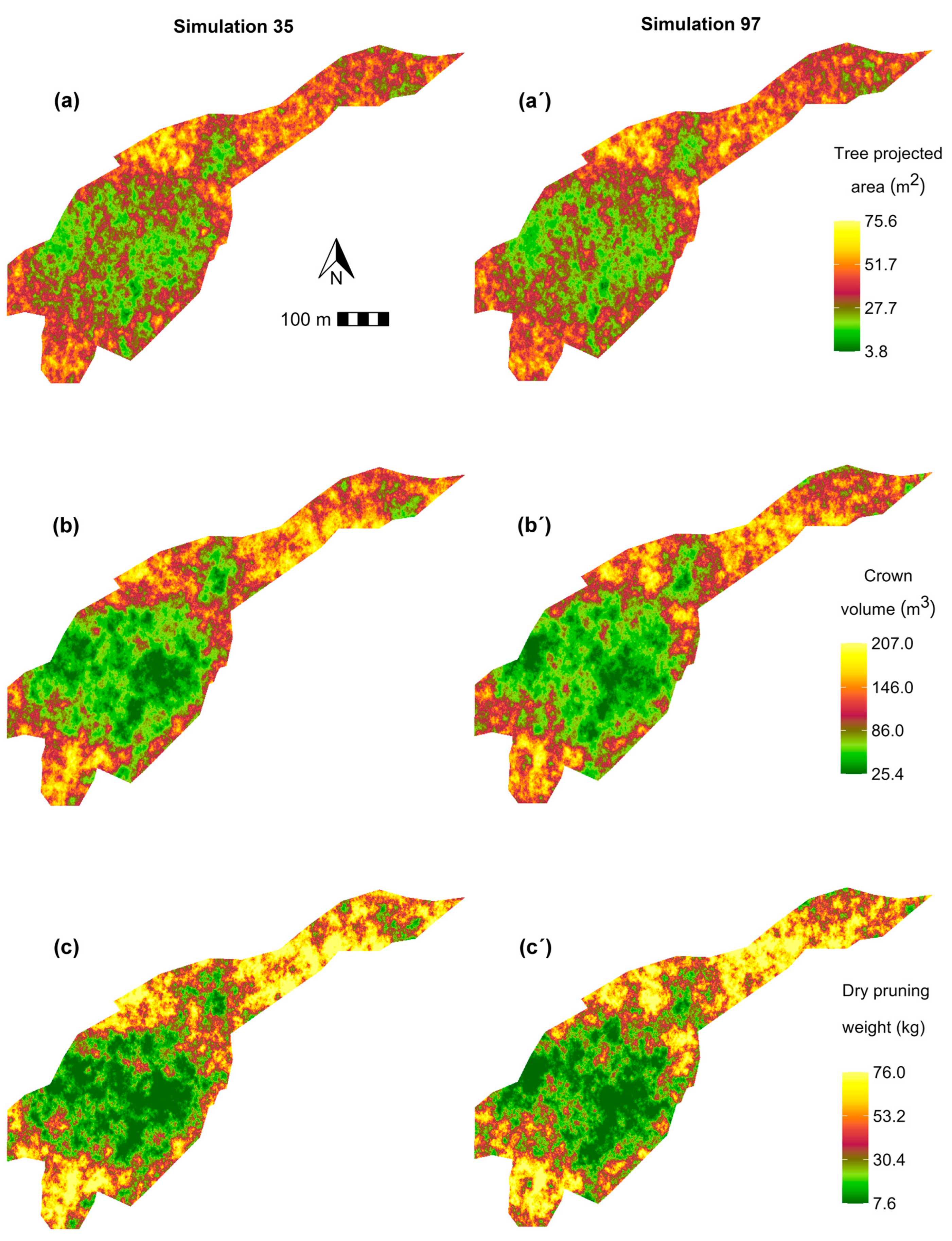
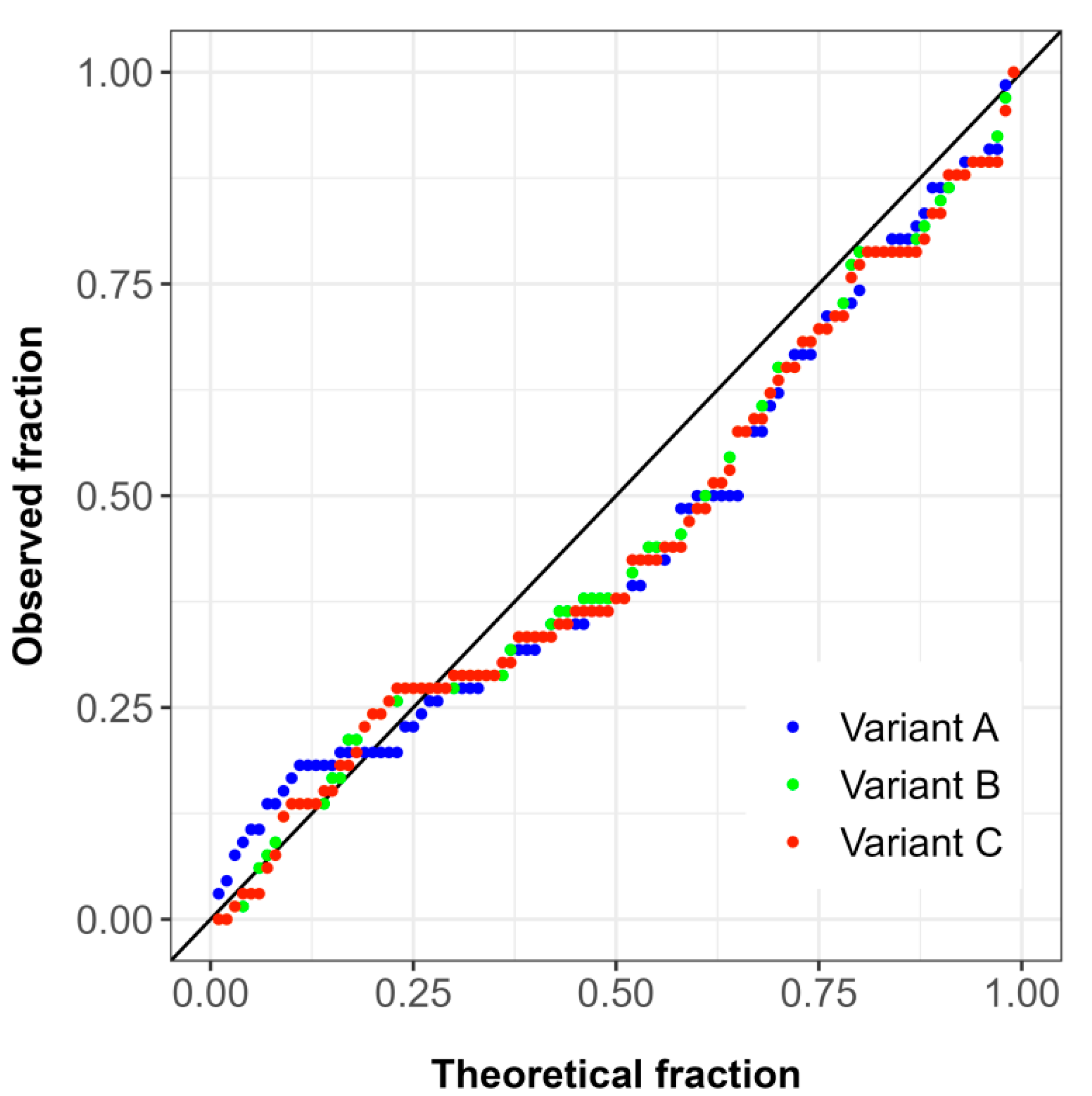
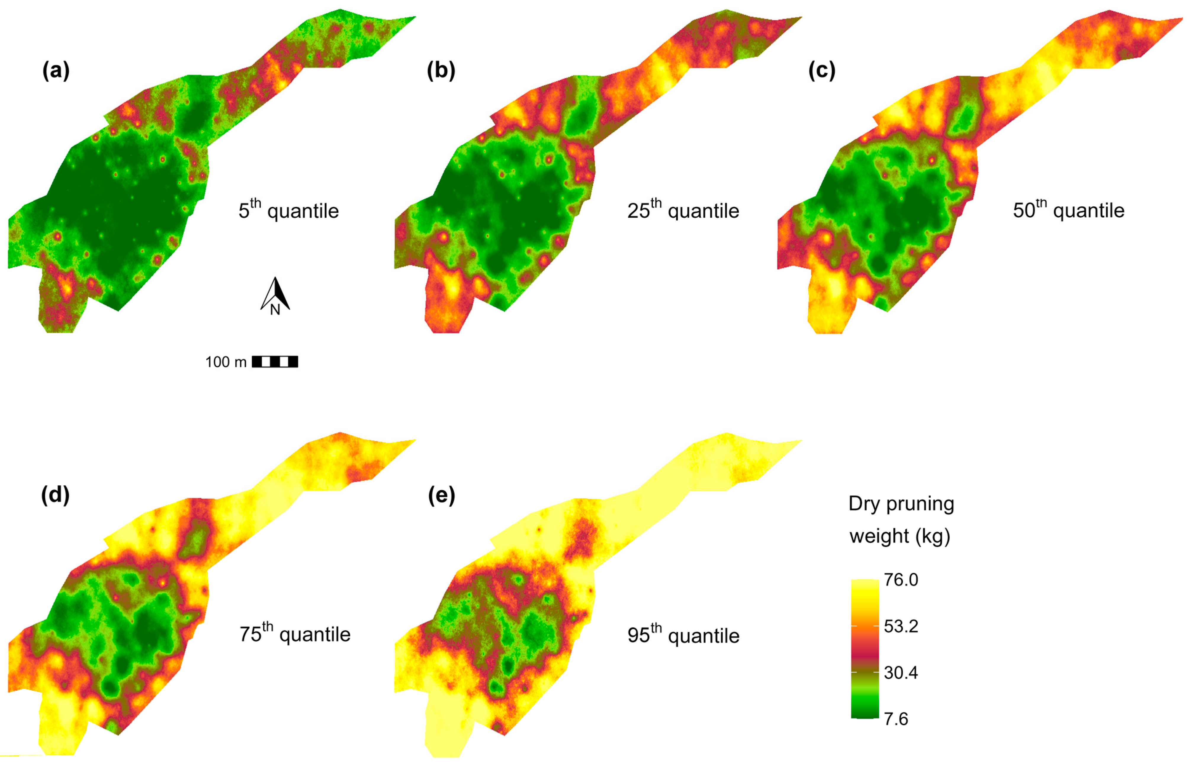
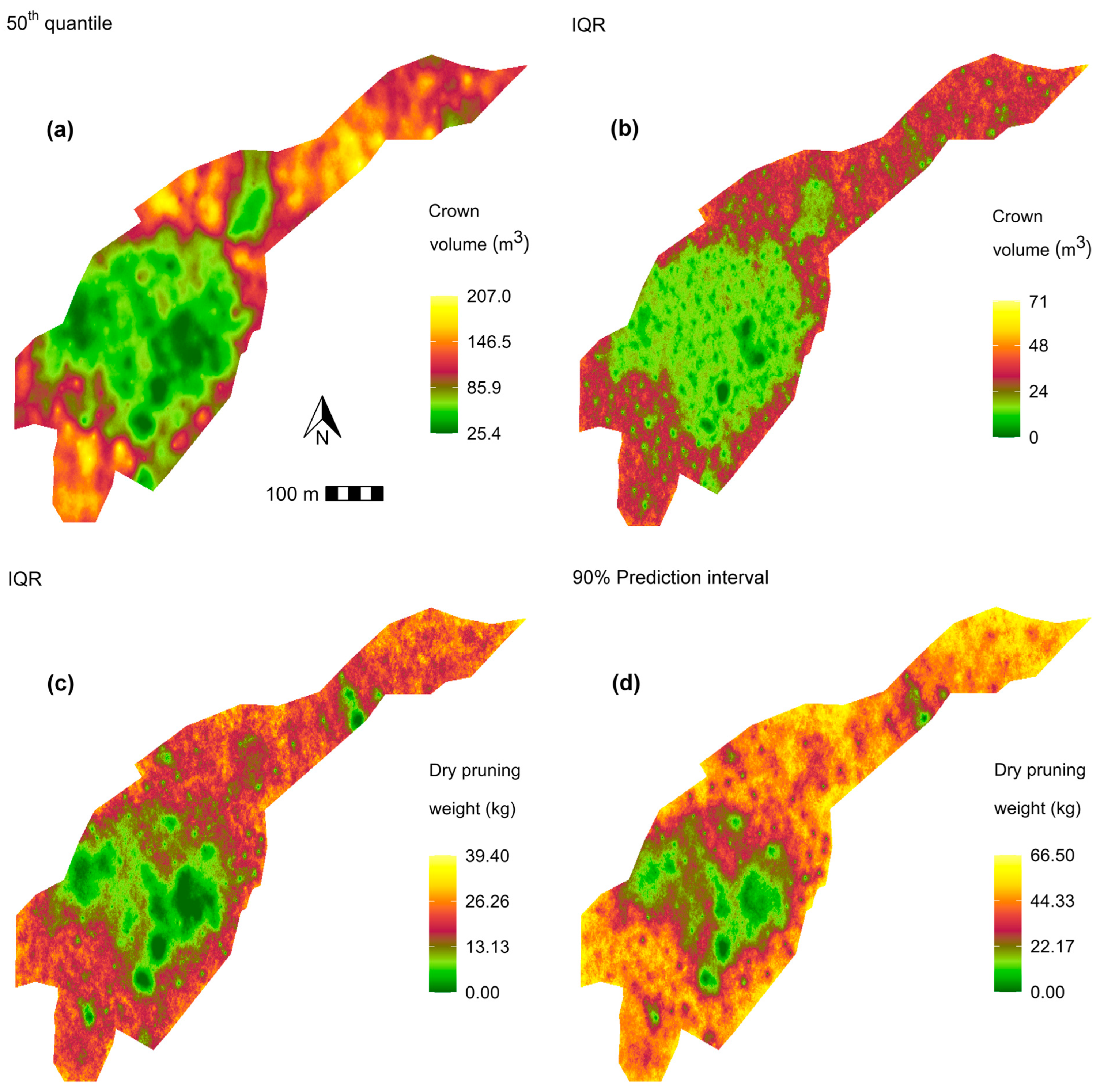
3.3. Spatial Uncertainty of Variables and Validation of Results

Stochastic simulations of the tree projected area were performed using DSS for variants A, B and C. CoDSS was used to generate images of the crown volume of the farm. Subsequently, the crown volume images were used as secondary information to obtain shreddable dry pruning weight images. DSS and CoDSS algorithms aim to reproduce the sample histogram and the variogram model of each variable, honoring conditioning data [45]. Figure 4 shows, by illustration, two realizations of the variables tree projected area (a, a′), crown volume (b, b′) and shreddable dry pruning weight (c, c′), obtained with the variograms of variant A. The visual similarity between images is due to the correlation coefficient between variables estimated from the field samples.

A total of one hundred and fifty images per variant were obtained for shreddable dry pruning weight. Techniques based on geostatistical simulation, intended to model spatial uncertainty, can be useful to get reliable information in those areas not sampled through the conditional cumulative distribution function at any node of the simulation grid [61,62].

Figure 5 shows the validation of the uncertainty quantifications using the accuracy plots for variants A, B and C, which present the scattergram of the estimated versus expected fractions. The quantification is found to be acceptable for the three sets of proposed variograms because the bisector is closely matched. The higher the value of G, the closer the observed and expected fractions will be [52]. Ideally, its value should be equal to one. The values of the goodness-of-fit statistic G were equal to 0.89, 0.90 and 0.89 for variants A, B and C, respectively. The variants show similar behavior for theoretical fractions higher than 0.25, although variant A performs somewhat better for large theoretical fractions. Thus, variant A was selected.

In this case, we have chosen to differentiate between underestimation and overestimation with different weights, following Deutsch [52] and later works. Szatmári et al. [63] propose to use the same weight in both cases because they understand that this benefits the purpose of using the G-statistic (Equation (4)). As additional information for the statistic, Wadoux et al. [47] determined the proportions of overestimation and underestimation based on the absolute deviation from the bisector.

The determination of the uncertainty related to the expected average values is of great importance in assessing risks in agronomic and environmental decision-making. Although the primary interest of map users often lies in the prediction map, relying solely on the visualization of the prediction can be misleading and may impart a false impression of the map’s quality. This can subsequently lead to biased decision-making processes. It is essential to quantify the uncertainty associated with the prediction to obtain a comprehensive understanding of the map’s quality. For this reason, the quantification of uncertainty is as important as the prediction itself [47]. If the uncertainty associated with the prediction is too large, users may choose to invest in acquiring a more accurate map.

The use of pruning images produced by stochastic simulation algorithms makes it possible to obtain a series of quantiles to be used for uncertainty estimation. Figure 6 shows the 5-th, 25-th, 50-th, 75-th and 95-th quantiles of the variable shreddable dry pruning weight. These quantiles allow for the use of prediction intervals (PI) [61,64,65,66]. The narrower the prediction intervals are, the lower the uncertainty of the estimate. The width of the 90% PI is a useful measure of the prediction uncertainty. The 90% PI reports the range of values within which the true value is expected to occur 9 times out of 10. Similarly, those areas where the difference between the quantiles is wider will reveal areas where there is less confidence in the estimate. Validating the uncertainty estimate is crucial and provides reliable information about the map’s quality. It is necessary for users to make informed decisions [47].

Figure 7a,b show the point predictions of crown volume in the study area, along with the quantified uncertainty of the predictions based on the interquartile range. Figure 7c,d show the quantified uncertainty for shreddable dry pruning weight, which is measured using the interquartile range as well as 90% PI.

It can be observed that both the interquartile range and the 90% PI of the shreddable dry pruning weight variable are small in the mid-western part of the farm and in a small area in the middle east. This may have implications for management decisions since in these locations there is high certainty that pruning weight will be much lower (mid-western area) or much higher (small area in the middle east) than in the rest of the farm (Figure 6c and Figure 7c,d). The figures also show areas where further investment in additional sampling may be necessary since the information is less reliable, for example, the eastern end of the farm. That happens because there is a propagation of uncertainty since the projected areas have high variability (Figure 2c), which results in a high interquartile range in the crown volume variable (Figure 7b) and, in turn, a high uncertainty of the estimate of shreddable dry pruning weight in that area (Figure 7c,d).

3.4. Agronomic and Energy Implications of the Spatial Distribution and Uncertainty of the Canopy Volume and Shreddable Pruning Material

The median value of the predicted crown volume per pixel in the farm is shown in Figure 7a. Understanding the spatial distribution of canopy volume is crucial for various agronomic applications, including the determination of appropriate doses for woody crop treatments [34,67], soil conservation [19], site-specific fertilization [56] and yield estimations [68]. In this sense, Örn [68] and Underwood et al. [69] indicated that the volume of the tree is the most important property for predicting fruit count. Likewise, variations in crown volume can affect harvesting efficiency [70], which makes it advisable to adapt the agricultural machinery to the canopy [71].

The median shreddable dry pruning weight is shown in Figure 6c. Olive pruning is a byproduct of the agro-industrial supply chain and not a virgin resource. Pruning can have two possible and opposing uses as a circular economy model. On the one hand, it can be applied to the soil to protect it and improve its properties, increasing soil C content, helping the climate with regulation and improving ecosystem services. On the other hand, it can be used for renewable energy generation, with the advantage of no additional soil demand, no negative impact on existing biodiversity and carbon neutrality. In this case, the service of pruning residues is provided outside the ecosystem where they were generated. This is the dilemma that Libuti et al. [72] refer to as “pruning to soil” or “pruning to energy”. As the authors point out, an impressive amount of energy can be obtained from pruning residues on a European scale. It is estimated that up to 3 Mt yr⁻¹ can be produced per year in Andalusia (Spain) [73].

For either of these two uses, it is necessary to know the potential amount of pruning on the farms. Estornell et al. [33] indicated that the use of airborne LiDAR sensors is feasible for pruning estimation in olive groves in a trial with 25 trees and two varieties of olive trees. Their pruning amounts ranged from 2.1 to 31 kg tree⁻¹, compared to the 7.6 to 76 kg tree⁻¹ in this study. However, it is necessary to determine its usefulness in large areas with different crops and plantation distances in isolated trees, as it would be helpful for the spatial determination of areas with higher or lower pruning rates in an agricultural field. Fernández-Sarría et al. [38] evaluated the amount of pruning in a sample of 32 trees, with strong relationships between residual biomass and crown volume parameters measured by TLS. The use of technologies such as satellite imagery, airborne LiDAR and UAVs allow for the estimation of dendrometric parameters and the determination of volume variation before and after pruning on a farm [35], which can be used as an auxiliary variable in dry pruning weight estimation. However, pruning biomass ground measurements are needed for field validation.

Similarly, it is necessary to obtain a measure of the associated uncertainty of shreddable pruning weight, which is fundamental when dealing with precision agriculture, as uncertainty varies from point to point and provides an idea of the confidence in the values obtained and the potential errors. Previous work [58] proposed linear regression models to estimate pruning quantities using some variables measured on the ground. However, they do not consider the spatial dimension as presented in this work. Thus, Velázquez et al. [58] and Fernández-Sarría et al. [38] present a global error in their models, which does not allow for establishing measures of uncertainty or zoning the farm.

In regards to “pruning to energy”, the knowledge of the areas with the highest biomass production potential could be used to locate biomass production plants, as stated by Torquati et al. [39]. In the last decade, the use of olive tree chips as fuel for electricity generation has experienced a significant increase due to the improved profitability for the service companies that commercialize it [73]. It is well-received as it is considered a green technology [74].

However, its use should be subject to careful economic and environmental analysis, as reported by Oyegoke et al. [75]. Several factors need to be considered, such as the spatial fragmentation of the crop, transportation costs, transfer costs, possible subsidies and legislation, in order to carefully analyze the economic and environmental impact of using olive tree chips as fuel. Studies have shown contrasting results on the economic profitability of these plants [39,75,76]. The Andalusian Government states that the profitability of biomass electricity generation is currently limited by existing legislation [73]. Nevertheless, in certain areas, acquiring olive pruning chips is more affordable than acquiring forest biomass, which has led to an increase in its consumption.

Regarding “pruning to soil”, pruning mulches have notable positive effects on soil. They improve the overall soil quality, increase soil organic C content [25] and porosity [77], reduce erosion and runoff, as well as diffuse pollution in runoff and sediments, increase soil infiltration capacity and reduce the appearance of weeds [22]. Recently, González-Ruiz et al. [27] have shown, using the olive moth (Prays oleae) as a bioindicator species, that the use of a spontaneous cover with pruning residues increases the diversity and abundance of beneficial insects, providing better results than conventional management or a spontaneous cover.

Similarly, pruning mulch results in the release of macronutrients, such as N, P and K [21]. Knowledge of the spatial variation in the amount of shreddable pruning provides insight into the variability of nutrients released at the farm level. This has implications for calculating fertilizer doses [78], which is crucial for crop productivity, both in terms of quantifying the amount of nutrients removed during pruning and the potential release of these nutrients over time. Understanding the spatial variability of factors that influence production is relevant for any precision system in olive groves [79].

However, the potential effects of mulch are often dependent on the mulching rate [77]. Thus, the increase in organic matter may be limited by the density of residues or may not be appreciable with small amounts of shreddable pruning. Taguas et al. [80] indicate that a minimum threshold of 7.5 $t{\mathrm{ha}}_{\mathrm{cover}}^{-1}$ is needed to observe the benefits of mulching on soil moisture. Likewise, a threshold of 15 $t{\mathrm{ha}}_{\mathrm{cover}}^{-1}$ of shreddable pruning residues to significantly increase soil C at 0–20 cm depth is needed [80]. For this reason, these authors recommend accumulating the mulch in rows with densities greater than 15 $t{\mathrm{ha}}_{\mathrm{cover}}^{-1}$ instead of using uniform distributions of greater width. The achievement of one or the other density will be conditioned by the amount of shreddable pruning available, as well as by the width of the cover. Similarly, the distribution of pruning in all rows of the plantation or in alternate rows alters the density in a 1:2 relationship. The latter is a common practice among farmers to increase the field performance of the shredding operation with agricultural machinery.

Knowledge of the amount of shreddable pruning residues existing in an agricultural field is also of interest for the proper use of agricultural machinery. The energy requirement of the agricultural chopping operation, its field performance and the size of the chopped residues depend largely on the amount of pruning biomass, as studied by Ortí [81] in citrus wood. Shredders or chippers require power between 70 and 150 kW [82]. Even though the average power is relatively low, the instantaneous torque peaks that appear in the shredding operation require high driving power. Thus, the superficial density of the mulch to be shredded will also influence the power required for the work, the speed of the machine’s advance and the working capacity of the shredding operation [59].

Likewise, a greater amount of shreddable pruning per tree implies greater soil coverage and therefore a higher sediment trapping efficiency [8]. The threshold value established in conservation agriculture to adequately maintain soil protection is 30% [83].

Therefore, given the presence of a series of thresholds for soil protection, agricultural mechanization, soil moisture and SOC, pruning mulches may be more useful in some areas of the farm than in others. Geostatistical techniques allow for zoning of the field based on these thresholds [61] using probabilistic determinations. This can enable the generation of simultaneous maps for various environmental variables related to the amount of mulch. In this way, it would be possible to determine in which parts of a farm this type of mulch could be especially beneficial.

4. Conclusions

There is significant natural variability in shreddable pruning amounts within farms. Tree crown volume, tree projected areas and shreddable pruning biomass are well correlated and display spatial autocorrelation. Thus, utilizing canopy volume and tree projected areas improves the spatial estimation of shreddable dry pruning weight, which is valuable for olive growers seeking to understand pruning variability on their farms.

However, relying solely on estimation can lead to biased decision-making. Incorporating prediction intervals provides complementary information for decision-making. A key finding of this study was the application of geostatistical methods and stochastic simulations to model the spatial variability and quantify the spatial uncertainty of olive pruning weight. This approach generates actionable information for olive growers. For instance, in the mid-western area of the farm, results indicate with high accuracy (narrow prediction interval) that shreddable dry pruning weight is significantly lower compared to other areas. Additionally, it is possible to confidently identify areas with a substantial amount of pruning mulch, which benefits olive growers by maintaining tree productivity, mitigating soil loss and runoff damage and improving soil quality.

The proposed methodology offers two advantages. Firstly, it integrates with any existing tree data measurement system, incorporating spatial patterns for more appropriate data treatment and providing spatial uncertainty assessment for the variables under study. This enhances a more robust analysis of the data and a better understanding of their spatial characteristics. Secondly, it can be scaled up to larger geographical areas by incorporating additional spatial data (such as measurements from other environmental factors related to pruning biomass) [84] and expanding geostatistical modeling with machine learning algorithms [64]. These expanded models can be applied to large regions, enabling the identification of areas with high biomass production and varying spatial uncertainty while avoiding fine-scale inference in regions with high uncertainty.

References

1. FAO Agricultural Statistics. Available online: http://faostat.fao.org (accessed on 23 January 2023).
2. Ministerio de Agricultura, Pesca y Alimentación. Anuario de Estadística. 2020. Available online: https://www.mapa.gob.es/es/estadistica/temas/publicaciones/anuario-de-estadistica/2020/default.aspx?parte=3&capitulo=07&grupo=12 (accessed on 3 June 2023).
3. Lucena, B.; Manrique, T.; Méndez, M.A. La olivicultura en el mundo y en España. In El Cultivo Del Olivo; Barranco, D., Fernández-Escobar, R., Rallo, L., Eds.; Ediciones MundiPrensa: Madrid, Spain, 2017; pp. 1–34. ISBN 9788484767145. [Google Scholar]
4. Parra, M.A. Suelo. In El Cultivo Del Olivo; Barranco, D., Fernández Escobar, R., Rallo, L., Eds.; Mundi-Prensa: Madrid, Spain, 2017; pp. 251–288. ISBN 9788484767145. [Google Scholar]
5. Fernández-Escobar, R.; de la Rosa, R.; León, L.; Gómez, J.A.; Testi, L.; Orgaz, F.; Gil-Ribes, J.A.; Quesada-Moraga, E.; Trapero, A.; Msallem, M. Sistemas de producción en olivicultura. Olivae Rev. Of. Cons. Oleícola Int. 2012, 118, 55–68. [Google Scholar]
6. Ministerio de Agricultura, Pesca y Alimentación. ESYRCE. Available online: https://www.mapa.gob.es/es/estadistica/temas/estadisticas-agrarias/agricultura/esyrce/ (accessed on 19 March 2023).
7. Saavedra, M.M.; Pastor, M. Sistemas de Cultivo en Olivar. Manejo de Malas Hierbas y Herbicidas; Editorial Agrícola Española: Madrid, Spain, 2002; ISBN 84-85441-65-6. [Google Scholar]
8. Espejo-Pérez, A.J.; Rodríguez-Lizana, A.; Ordóñez, R.; Giráldez, J.V. Soil Loss and Runoff Reduction in Olive-Tree Dry-Farming with Cover Crops. Soil Sci. Soc. Am. J. 2013, 77, 2140–2148. [Google Scholar] [CrossRef] [Green Version]
9. Cerdà, A.; Lavee, H.; Romero-Díaz, A.; Hooke, J.; Montanarella, L. Soil erosion and degradation in Mediterranean-type ecosystems. L. Degrad. Dev. 2010, 21, 71–74. [Google Scholar] [CrossRef]
10. Panagos, P.; Borrelli, P.; Poesen, J.; Ballabio, C.; Lugato, E.; Meusburger, K.; Montanarella, L.; Alewell, C. The new assessment of soil loss by water erosion in Europe. Environ. Sci. Policy 2015, 54, 438–447. [Google Scholar] [CrossRef]
11. Ordóñez-Fernández, R.; Repullo-Ruibérriz de Torres, M.A.; Márquez-García, J.; Moreno-García, M.; Carbonell-Bojollo, R.M. Legumes used as cover crops to reduce fertilisation problems improving soil nitrate in an organic orchard. Eur. J. Agron. 2018, 95, 1–13. [Google Scholar] [CrossRef]
12. Torrús-Castillo, M.; Domouso, P.; Herrera-Rodríguez, J.M.; Calero, J.; García-Ruiz, R. Aboveground Carbon Fixation and Nutrient Retention in Temporary Spontaneous Cover Crops in Olive Groves of Andalusia. Front. Environ. Sci. 2022, 10, 868410. [Google Scholar] [CrossRef]
13. Rodríguez-Lizana, A.; Repullo-Ruibérriz De Torres, M.A.; Carbonell-Bojollo, R.; Alcántara, C.; Ordóñez-Fernández, R. Brachypodium distachyon, Sinapis alba, and controlled spontaneous vegetation as groundcovers: Soil protection and modeling decomposition. Agric. Ecosyst. Environ. 2018, 265, 62–72. [Google Scholar] [CrossRef]
14. Alcántara, C.; Pujadas, A.; Saavedra, M. Management of cruciferous cover crops by mowing for soil and water conservation in southern Spain. Agric. Water Manag. 2011, 98, 1071–1080. [Google Scholar] [CrossRef]
15. Rodríguez-Lizana, A.; Repullo-Ruibérriz de Torres, M.A.; Carbonell-Bojollo, R.M.; Moreno-García, M.; Ordóñez-Fernández, R. Study of C, N, P and K Release from Residues of Newly Proposed Cover Crops in a Spanish Olive Grove. Agronomy 2020, 10, 1041. [Google Scholar] [CrossRef]
16. Repullo-Ruibérriz de Torres, M.A.; Carbonell-Bojollo, R.M.; Moreno-García, M.; Ordóñez-Fernández, R.; Rodríguez-Lizana, A. Soil organic matter and nutrient improvement through cover crops in a Mediterranean olive orchard. Soil Tillage Res. 2021, 210, 104977. [Google Scholar] [CrossRef]
17. Hao, X.; Abou, M.; Steenwerth, K.L.; Nocco, M.A.; Basset, C.; Daccache, A. Are there universal soil responses to cover cropping? A systematic review. Sci. Total Environ. 2023, 861, 160600. [Google Scholar] [CrossRef]
18. Rodríguez-Lizana, A.; Espejo-Pérez, A.J.; González-Fernández, P.; Ordóñez-Fernández, R. Pruning residues as an alternative to traditional tillage to reduce erosion and pollutant dispersion in olive groves. Water Air Soil Pollut. 2008, 193, 165–173. [Google Scholar] [CrossRef]
19. Rodríguez-Lizana, A.; Pereira, M.J.; Ribeiro, M.C.; Soares, A.; Márquez-García, F.; Ramos, A.; Gil-Ribes, J. Assessing Local Uncertainty of Soil Protection in an Olive Grove Area with Pruning Residues Cover: A Geostatistical Cosimulation Approach. Land Degrad. Dev. 2017, 28, 2086–2097. [Google Scholar] [CrossRef]
20. Repullo, M.A.; Carbonell, R.; Hidalgo, J.; Rodríguez-Lizana, A.; Ordóñez, R. Using olive pruning residues to cover soil and improve fertility. Soil Tillage Res. 2012, 124, 36–46. [Google Scholar] [CrossRef]
21. Ordóñez-Fernández, R.; Repullo-Ruibérriz de Torres, M.A.; Román-Vázquez, J.; González-Fernández, P.; Carbonell-Bojollo, R. Macronutrients released during the decomposition of pruning residues used as plant cover and their effect on soil fertility. J. Agric. Sci. 2015, 153, 615–630. [Google Scholar] [CrossRef]
22. Henry, G.M.; Hoyle, J.A.; Beck, L.L.; Cooper, T.; Montague, T.; Mckenney, C. Evaluation of Mulch and Preemergence Herbicide Combinations for Weed Control in High-density Olive (Olea europaea L.) Production. HortScience 2015, 50, 1338–1341. [Google Scholar] [CrossRef]
23. López-Escudero, F.J.; Mercado-Blanco, J. Verticillium wilt of olive: A case study to implement an integrated strategy to control a soil-borne pathogen. Plant Soil 2011, 344, 1–50. [Google Scholar] [CrossRef] [Green Version]
24. Mairech, H.; López-Bernal, Á.; Moriondo, M.; Dibari, C.; Regni, L.; Proietti, P.; Villalobos, F.J.; Testi, L. Is new olive farming sustainable? A spatial comparison of productive and environmental performances between traditional and new olive orchards with the model OliveCan. Agric. Syst. 2020, 181, 102816. [Google Scholar] [CrossRef]
25. Gómez-Muñoz, B.; Valero-Valenzuela, J.D.; Hinojosa, M.B.; García-Ruiz, R. Management of tree pruning residues to improve soil organic carbon in olive groves. Eur. J. Soil Biol. 2016, 74, 104–113. [Google Scholar] [CrossRef]
26. Nieto, O.M.; Castro, J.; Fernández, E.; Smith, P. Simulation of soil organic carbon stocks in a Mediterranean olive grove under different soil-management systems using the RothC model. Soil Use Manag. 2010, 26, 118–125. [Google Scholar] [CrossRef]
27. González-Ruiz, R.; Gómez-Guzmán, A.; Martínez-Rojas, M.; García-Fuentes, A.; Cordovilla, M.; Sainz-Pérez, M.; Sánchez-Solana, A.; Rodríguez-Lizana, A. The Influence of Mixed Green Covers, a New Trend in Organic Olive Growing, on the Efficiency of Predatory Insects. Agriculture 2023, 13, 785. [Google Scholar] [CrossRef]
28. Calatrava, J.; Franco, J.A. Using pruning residues as mulch: Analysis of its adoption and process of diffusion in Southern Spain olive orchards. J. Environ. Manag. 2011, 92, 620–629. [Google Scholar] [CrossRef]
29. Boletín Oficial del Estado. Ley 7/2022, de 8 de Abril, de Residuos y Suelos Contaminados Para Una Economía Circular; State Agency Official State Gazette: Madrid, Spain, 2022; pp. 1–136. [Google Scholar]
30. Moreno-García, M.; Repullo-Ruibérriz de Torres, M.A.; Carbonell-Bojollo, R.M.; Ordóñez-Fernández, R. Management of pruning residues for soil protection in olive orchards. Land Degrad. Dev. 2018, 29, 2975–2984. [Google Scholar] [CrossRef]
31. Manzanares, P.; Ruiz, E.; Ballesteros, M.; Negro, M.J. Residual biomass potential in olive tree cultivation and olive oil industry in Spain: Valorization proposal in a biorefinery context. Span. J. Agric. Res. 2017, 15, 6. [Google Scholar] [CrossRef] [Green Version]
32. Li, R.; Li, Q.; Pan, L. Review of organic mulching effects on soil and water loss. Arch. Agron. Soil Sci. 2021, 67, 136–151. [Google Scholar] [CrossRef]
33. Estornell, J.; Ruiz, L.A.; Velázquez-Martí, B.; López-Cortés, I.; Salazar, D.; Fernández-Sarría, A. Estimation of pruning biomass of olive trees using airborne discrete-return LiDAR data. Biomass Bioenergy 2015, 81, 315–321. [Google Scholar] [CrossRef]
34. Rodríguez-Lizana, A.; Pereira, M.J.; Ribeiro, M.C.; Soares, A.; Azevedo, L.; Miranda-Fuentes, A.; Llorens, J. Spatially variable pesticide application in olive groves: Evaluation of potential pesticide-savings through stochastic spatial simulation algorithms. Sci. Total Environ. 2021, 778, 146111. [Google Scholar] [CrossRef]
35. Jiménez-Brenes, F.M.; López-Granados, F.; Castro, A.I.; Torres-Sánchez, J.; Serrano, N.; Peña, J.M. Quantifying pruning impacts on olive tree architecture and annual canopy growth by using UAV-based 3D modelling. Plant Methods 2017, 13, 55. [Google Scholar] [CrossRef] [Green Version]
36. Velàzquez-Martì, B.; Cortès, I.L.; Salazar-Hernàndez, D.M. Dendrometric analysis of olive trees for wood biomass quantification in Mediterranean orchards. Agrofor. Syst. 2014, 88, 755–765. [Google Scholar] [CrossRef]
37. Assirelli, A.; Romano, E.; Bisaglia, C.; Lodolini, E.M.; Neri, D.; Brambilla, M. Canopy Index Evaluation for Precision Management in an Intensive Olive Orchard. Sustainability 2021, 13, 8266. [Google Scholar] [CrossRef]
38. Fernández-Sarría, A.; López-Cortés, I.; Estornell, J.; Velázquez-Martí, B.; Salazar, D. Estimating residual biomass of olive tree crops using terrestrial laser scanning. Int. J. Appl. Earth Obs. Geoinf. 2019, 75, 163–170. [Google Scholar] [CrossRef]
39. Torquati, B.; Marino, D.; Venanzi, S.; Porceddu, P.R.; Chiorri, M. Using tree crop pruning residues for energy purposes: A spatial analysis and an evaluation of the economic and environmental sustainability. Biomass Bioenergy 2016, 95, 124–131. [Google Scholar] [CrossRef]
40. Fernández-Sarría, A.; López-Cortés, I.; Martí, J.; Estornell, J. Estimation of Walnut Structure Parameters Using Terrestrial Photogrammetry Based on Structure-from-Motion (SfM). J. Indian Soc. Remote Sens. 2022, 50, 1931–1944. [Google Scholar] [CrossRef]
41. Méndez, V.; Pérez-Romero, A.; Sola-Guirado, R.R.; Miranda-Fuentes, A.; Manzano-Agugliaro, F.; Zapata-Sierra, A.; Rodríguez-Lizana, A. In-Field Estimation of Orange Number and Size by 3D Laser Scanning. Agronomy 2019, 9, 885. [Google Scholar] [CrossRef] [Green Version]
42. Escolà, A.; Martínez-Casasnovas, J.A.; Rufat, J.; Arnó, J.; Arbonés, A.; Sebé, F.; Pascual, M.; Gregorio, E.; Rosell-Polo, J.R. Mobile terrestrial laser scanner applications in precision fruticulture/horticulture and tools to extract information from canopy point clouds. Precis. Agric. 2017, 18, 111–132. [Google Scholar] [CrossRef] [Green Version]
43. Dalla Corte, A.P.; Rex, F.E.; Roberti, D.; De Almeida, A.; Sanquetta, C.R.; Silva, C.A.; Moura, M.M.; Wilkinson, B.; Maria, A.; Zambrano, A.; et al. Measuring Individual Tree Diameter and Height Using GatorEye High-Density UAV-Lidar in an Integrated Crop-Livestock-Forest System. Remote Sens. 2020, 12, 863. [Google Scholar] [CrossRef] [Green Version]
44. Cambardella, C.A.; Moorman, T.B.; Novak, J.M.; Parkin, T.B.; Karlen, D.L.; Turco, R.F.; Konopka, A.E. Field-scale variability of soil properties in Central Iowa soils. Soil Sci. Soc. Am. J. 1994, 58, 1501–1511. [Google Scholar] [CrossRef]
45. Soares, A. Direct Sequential Simulation and Cosimulation. Math. Geol. 2001, 33, 911–926. [Google Scholar] [CrossRef]
46. Horta, A.; Soares, A. Direct sequential Co-simulation with joint probability distributions. Math. Geosci. 2010, 42, 269–292. [Google Scholar] [CrossRef]
47. Wadoux, A.M.J.; Brus, D.J.; Heuvelink, G.B.M. Accounting for non-stationary variance in geostatistical mapping of soil properties. Geoderma 2018, 324, 138–147. [Google Scholar] [CrossRef]
48. Peel, M.; Fynlaison, B.; McMahon, T. Updated world map of the Köppen-Geiger classification. Hydrol. Earth Syst. Sci. 2007, 11, 1633–1644. [Google Scholar] [CrossRef] [Green Version]
49. Agencia Estatal de Meteorología. Valores Climáticos Normales. Available online: https://www.aemet.es/es/serviciosclimaticos/datosclimatologicos/valoresclimatologicos (accessed on 15 June 2023).
50. Panagiotou, C.F.; Kyriakidis, P.; Tziritis, E. Application of geostatistical methods to groundwater salinization problems: A review. J. Hydrol. 2022, 615, 128566. [Google Scholar] [CrossRef]
51. Goovaerts, P. Geostatistics for Natural Resources Evaluation; Oxford University Press: Oxford, UK, 1997. [Google Scholar]
52. Deutsch, C. V Direct assessment of local accuracy and precision. In Proceedings of the Geostatistics Wollongong ’96, Wollongong, Australia, 2–6 September 1996; Baafi, E.Y., Schofield, N.A., Eds.; Kluwer Academic Publishing: Dordrecht, The Netherlands, 1997; pp. 115–125. [Google Scholar]
53. R Core Team R: A Language and Environment for Statistical Computing 2019; R Foundation for Statistical Computing: Vienna, Austria. Available online: https://www.R-project.org/ (accessed on 3 June 2023).
54. Schneider, C.A.; Rasband, W.S.; Eliceiri, K.W. Historical commentary NIH Image to ImageJ: 25 years of image analysis. Nat. Methods 2012, 9, 671–675. [Google Scholar] [CrossRef] [PubMed]
55. Miranda-Fuentes, A.; Llorens, J.; Gamarra-Diezma, J.; Gil-Ribes, J.; Gil, E. Towards an Optimized Method of Olive Tree Crown Volume Measurement. Sensors 2015, 15, 3671–3687. [Google Scholar] [CrossRef] [PubMed] [Green Version]
56. Schumman, A.; Hostler, K.; Buchanon, S.; Zaman, Q. Relating citrus canopy size and yield to precision fertilization. Proc. Fla. State Hortic. Soc. 2006, 119, 148–154. [Google Scholar]
57. Jopaul, G.; Panzou, L.; Fayolle, A.; Jucker, T.; Phillips, O.L.; Bohlman, S.; Banin, L.F.; Lewis, S.L.; Luciana, K.A.; Cécile, F.A.; et al. Pantropical variability in tree crown allometry. Glob. Ecol. Biogeogr. 2021, 30, 459–475. [Google Scholar]
58. Velázquez-Martí, B.; Fernández-González, E.; López-Cortés, I.; Salazar-Hernández, D.M. Quantification of the residual biomass obtained from pruning of trees in Mediterranean olive groves. Biomass Bioenergy 2011, 35, 3453–3464. [Google Scholar] [CrossRef]
59. Castillo-Ruiz, F.J.; Sola-Guirado, R.; Castro-García, S.; González-Sánchez, E.J.; Colmenero-Martínez, J.T.; Blanco-Roldán, G.L. Scientia Horticulturae Pruning systems to adapt traditional olive orchards to new integral harvesters. Sci. Hortic. 2017, 220, 122–129. [Google Scholar] [CrossRef]
60. Colaço, A.F.; Molin, J.P.; Rosell-Polo, J.R.; Escolà, A. Spatial variability in commercial orange groves. Part 1: Canopy volume and height. Precis. Agric. 2019, 20, 805–822. [Google Scholar] [CrossRef] [Green Version]
61. Goovaerts, P. Geostatistical modelling of uncertainty in soil science. Geoderma 2001, 103, 3–26. [Google Scholar] [CrossRef]
62. Chilès, J.-P.; Delfiner, P. Geostatistics. Modelling Spatial Uncertainty, 2nd ed.; John Wiley & Sons, Inc.: Hoboken, NJ, USA, 2012; ISBN 978-0-470-18315-1. [Google Scholar]
63. Szatmári, G.; Bakacsi, Z.; Laborczi, A.; Petrik, O.; Pataki, R.; Tóth, T.; Pásztor, L. Elaborating Hungarian Segment of the Global Map of Salt-Affected Soils (GSSmap): National Contribution to an International Initiative. Remote Sens. 2020, 12, 4073. [Google Scholar] [CrossRef]
64. Szatmári, G.; Pásztor, L.; Heuvelink, G.B.M. Estimating soil organic carbon stock change at multiple scales using machine learning and multivariate geostatistics. Geoderma 2021, 403, 115356. [Google Scholar] [CrossRef]
65. Sun, X.L.; Zhao, Y.G.; Wu, Y.J.; Zhao, M.S.; Wang, H.L.; Zhang, G.L. Spatio-temporal change of soil organic matter content of Jiangsu Province, China, based on digital soil maps. Soil Use Manag. 2012, 28, 318–328. [Google Scholar] [CrossRef]
66. Allocca, C.; Castrignanò, A.; Nasta, P.; Romano, N. Geoderma Regional-scale assessment of soil functions and resilience indicators: Accounting for change of support to estimate primary soil properties and their uncertainty. Geoderma 2023, 431, 116339. [Google Scholar] [CrossRef]
67. Miranda-Fuentes, A.; Llorens, J.; Rodríguez-Lizana, A.; Cuenca, A.; Gil, E.; Blanco-Roldán, G.L.; Gil-Ribes, J.A. Assessing the optimal liquid volume to be sprayed on isolated olive trees according to their canopy volumes. Sci. Total Environ. 2016, 568, 296–305. [Google Scholar] [CrossRef]
68. Örn, S. Estimating Light Interception of Orchard Trees Using LiDAR and Solar Models; Linköoping University: Linköping, Sweden, 2016. [Google Scholar]
69. Underwood, J.P.; Hung, C.; Whelan, B.; Sukkarieh, S. Mapping almond orchard canopy volume, flowers, fruit and yield using lidar and vision sensors. Comput. Electron. Agric. 2016, 130, 83–96. [Google Scholar] [CrossRef]
70. Maldera, F.; Vivaldi, G.A.; Iglesias-castellarnau, I.; Camposeo, S. Two Almond Cultivars Trained in a Super-High Density Orchard Show Different Growth, Yield Efficiencies and Damages by Mechanical Harvesting. Agronomy 2021, 11, 1406. [Google Scholar] [CrossRef]
71. Sola-Guirado, R.R.; Bayano-Tejero, S.; Rodríguez-Lizana, A.; Gil-Ribes, J.A.; Miranda-Fuentes, A. Assessment of the Accuracy of a Multi-Beam LED Scanner Sensor for Measuring Olive Canopies. Sensors 2018, 18, 4406. [Google Scholar] [CrossRef] [Green Version]
72. Libutti, A.; Rita, A.; Cammerino, B.; Monteleone, M. Management of Residues from Fruit Tree Pruning: A Trade-Off between Soil Quality and Energy Use. Agronomy 2021, 11, 236. [Google Scholar] [CrossRef]
73. De Andalucía, J. La bioenergia en Andalucía; Sevilla, Spain. 2020. Available online: https://www.agenciaandaluzadelaenergia.es/sites/default/files/Documentos/3_2_0068_20_LA_BIOENERGIA_EN_ANDALUCIA.PDF (accessed on 23 January 2023).
74. Adeleke, A.A.; Ikubanni, P.P.; Orhadahwe, T.A.; Christopher, C.T.; Akano, J.M.; Agboola, O.O.; Adegoke, S.O.; Balogun, A.O.; Ibikunle, R.A. Heliyon Sustainability of multifaceted usage of biomass: A review. Heliyon 2021, 7, e08025. [Google Scholar] [CrossRef]
75. Oyegoke, T.; Obadiah, E.; Mohammed, S.Y.; Bamigbala, O.A.; Owolabi, O.A.; Oyegoke, A.; Onadeji, A.; Mantu, A.I. Papers of the 29th European Biomass Conference Setting the course for a biobased economy. In Proceedings of the Exploration Of Biomass for the Production of Bioethanol: “Economic Feasibility and Optimization Studies of Transforming Maize Cob into Bioethanol as a Substitute for Fossil Fuels” Conference, Online, 26–29 April 2021; Mauguin, P., Scarlat, N., Grassi, A., Eds.; pp. 1270–1275. [Google Scholar]
76. Palmieri, N.; Suardi, A.; Alfano, V.; Pari, L. Circular Economy Model: Insights from a Case Study in South Italy. Sustainability 2020, 12, 3466. [Google Scholar] [CrossRef] [Green Version]
77. Jordán, A.; Zavala, L.M.; Gil, J. Catena Effects of mulching on soil physical properties and runoff under semi-arid conditions in southern Spain. Catena 2010, 81, 77–85. [Google Scholar] [CrossRef]
78. Rodrigues, M.Â.; Ferreira, I.Q.; Marília, A.; Arrobas, M. Scientia Horticulturae Fertilizer recommendations for olive based upon nutrients removed in crop and pruning. Sci. Hortic. 2012, 142, 205–211. [Google Scholar] [CrossRef]
79. Silveira, C.; Almeida, A.; Ribeiro, C. Technological Innovation in the Traditional Olive Orchard Management: Advances and Opportunities to the Northeastern Region of Portugal. Water 2022, 14, 4081. [Google Scholar] [CrossRef]
80. Taguas, V.; Marín-Moreno, V.; Barranco, D.; Rafael, P.; García-ferrer, A. Opportunities of super high-density olive orchard to improve soil quality: Management guidelines for application of pruning residues. J. Environ. Manage. 2021, 293, 112785. [Google Scholar] [CrossRef]
81. Ortí, E. Determinación y Análisis de Las Condiciones Óptimas de Trabajo de Una Trituradora de eje Horizontal Sobre Restos de Poda de Cítricos; Universidad Politécnica de Valéncia: València, Spain, 2001. [Google Scholar]
82. Pari, L.; Suardi, A.; Santangelo, E.; García-galindo, D.; Scarfone, A.; Alfano, V. Biomass and Bioenergy Current and innovative technologies for pruning harvesting: A review. Biomass Bioenergy 2017, 107, 398–410. [Google Scholar] [CrossRef]
83. Conservation Tillage Information Center Tillage Type Definitions. Available online: https://www.extension.purdue.edu/extmedia/ct/ct-1.html (accessed on 27 March 2023).
84. Buttafuoco, G.; Caloiero, T.; Coscarelli, R. Spatial uncertainty assessment in modelling reference evapotranspiration at regional scale. Hydrol. Earth Syst. Sci. 2010, 14, 2319–2327. [Google Scholar] [CrossRef] [Green Version]
Figure 1. (A) Location of field trial in Córdoba (south of Spain). (B) Study domain: traditional olive grove farm.
Agronomy 13 01697 g001
Figure 2. Spatial location of the field samples—crown volume (a) and shreddable dry pruning weight (b)—and laboratory measurements—tree projected area (c)—in the study area.
Agronomy 13 01697 g002
Figure 3. Experimental semiovariograms (dots) and fitted models (black solid lines) for tree projected area, crown volume and shreddable dry pruning weight. For each variable, the letters A, B and C refer to each of the 3 variants used in the study. The numbers 1, 2 and 3 refer to the variables tree projected area, crown volume and shreddable dry pruning weight, respectively.
Agronomy 13 01697 g003
Figure 4. Two examples of simulated images of tree projected area (a,a′), crown volume (b,b′) and shreddable dry pruning weight (c,c′).
Agronomy 13 01697 g004
Figure 5. Accuracy plot for shreddable dry pruning weight in variants A, B and C. The plot shows the graphical technique used to check if the proportions of simulated values with each variant (y-axis) match the theoretical quantiles within a specified probability (x-axis). If the proportions of simulated values were similar to observed ones in all quantiles, the points would fall along the bisecting line (45-degree reference line).
Agronomy 13 01697 g005
Figure 6. Spatial uncertainty of shreddable dry pruning weight in the study domain based on direct sequential cosimulation images. The maps show the spatial distribution of shreddable dry pruning weight in the study domain for the (a) 5-th, (b) 25-th, (c) 50-th, (d) 75-th and (e) 95-th quantiles.
Agronomy 13 01697 g006
Figure 7. Spatial uncertainty derived from direct sequential cosimulation images of field variables: (a,b) 50-th quantile and interquartile range of crown volume; and (c,d) interquartile range and 90% prediction interval of shreddable dry pruning weight.
Agronomy 13 01697 g007