Leveraging Hyperspectral Images for Accurate Insect Classification with a Novel Two-Branch Self-Correlation Approach

Abstract

Insect recognition, crucial for agriculture and ecology studies, benefits from advancements in RGB image-based deep learning, yet still confronts accuracy challenges. To address this gap, the HI30 dataset is introduced, comprising 2115 hyperspectral images across 30 insect categories, which offers richer information than RGB data for enhancing classification accuracy. To effectively harness this dataset, this study presents the Two-Branch Self-Correlation Network (TBSCN), a novel approach that combines spectrum correlation and random patch correlation branches to exploit both spectral and spatial information. The effectiveness of the HI30 and TBSCN is demonstrated through comprehensive testing. Notably, while ImageNet-pre-trained networks adapted to hyperspectral data achieved an 81.32% accuracy, models developed from scratch with the HI30 dataset saw a substantial 9% increase in performance. Furthermore, applying TBSCN to hyperspectral data raised the accuracy to 93.96%. Extensive testing confirms the superiority of hyperspectral data and validates TBSCN’s efficacy and robustness, significantly advancing insect classification and demonstrating these tools’ potential to enhance precision and reliability.

1. Introduction

Accurately identifying insects has profound significance in contemporary society, particularly within the realms of agriculture and economy, as it influences strategies for pest management, crop protection, and sustainable economic development. Firstly, insects are the most diverse and widely distributed biological community on earth [1], playing an important role in the stability and function of ecosystems. Secondly, accurately identifying insects can help develop better strategies to reduce risks, protect crops, and ensure sustainable economic growth. More specifically, it helps agricultural workers take timely and appropriate measures to protect crops from pests and reduce crop losses. On the other hand, beneficial insects such as bees and ladybugs promote agricultural production and need to be recognized. Furthermore, by judging whether insects are beneficial to human society based on their value, policymakers and economists can make wise decisions in pest control, resource allocation, and risk management [2]. For example, identifying invasive species, preventing the spread of pests and diseases, and controlling fruit flies or weevils in food cannot only prevent pollution but also help ensure food safety.

In the pre-technology era, people mainly relied on the professional knowledge of entomologists to identify insects. The methods employed by experts to identify and classify insects were reliable but slow, observing the morphological characteristics of insects, such as wing shape, color, and antennae. Based on existing visual insect recognition research in recent years, with the development of visual insect recognition research, this study briefly divides these works into legal computer vision technology-based and deep learning-based methods. Traditional computer vision methods, exemplified by works such as [3,4], rely on feature extraction and automated classification, but they often exhibit lower accuracy or limited generalization. By contrast, applying deep learning based on convolutional neural networks (CNNs) to insect recognition can more accurately identify insects without the need for manual feature extraction. However, insect recognition methods based on deep learning require high-quality datasets. In the field of agricultural pest and disease control, much work has been devoted to constructing and researching relevant datasets [5,6,7,8,9,10,11,12]. However, some works only focus on specific species or domains, such as Tiger Beetle [9], Deng et al. [5], Alfaris et al. [6], and Kusrini et al. [11]. The most prominent example among these tasks is IP102 [7], which provides a dataset source or baseline for many insect classification algorithms [13,14]. Acquiring data on insects poses challenges, and currently, insect classification usually only considers RGB to identify insects. The reliance on RGB data, which only captures information across three channels (red, green, and blue), inherently limits the depth of spectral information that can be gathered. Given the subtle variations in texture and color among different insect species, RGB-based classification methods may struggle to effectively distinguish between them. However, hyperspectral imaging provides a solution by providing rich spectral information in multiple bands. This allows for a more comprehensive representation of insect features; even with the same number of samples, richer features can be extracted.

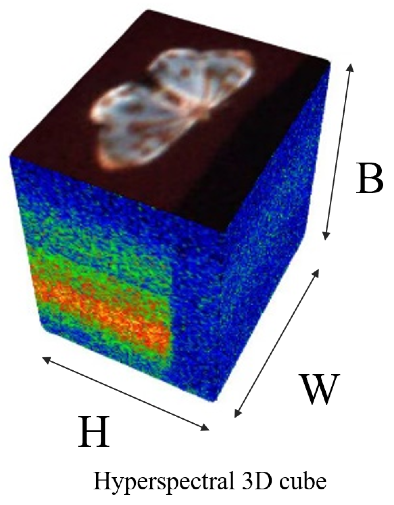
Spectra are the intensities of light reflected, emitted, or projected by an object at different wavelengths. Unlike traditional color imaging techniques, hyperspectral imaging captures the spectral information of a target object in hundreds of consecutive and dense spectra, thus providing a continuous spectral profile or spectral signature (Spectral signature means that the molecular structure of each substance has unique absorption and reflection properties for specific wavelengths of light, which gives rise to the “spectral signature”) for each pixel. A three-dimensional (3D) data cube can be obtained through hyperspectral equipment. Two spatial dimensions represent the width and height of the image, while the third dimension represents the spectral dimension (wavelength). Each spatial pixel has a spectral vector representing its reflectance, emissivity, and projection characteristics at all wavelengths, as seen in Figure 1.

Hyperspectral image classification typically refers to the classification of pixels in hyperspectral images based on their spectral characteristics in multiple narrow and continuous spectral bands. Common strategies in hyperspectral classification tasks include feature selection [15], feature extraction [16], grayscale co-occurrence matrix [17], and Gabor filters [18]. Techniques like tLTSL [19] and $L_{2,p}$-RER [20] introduce innovative techniques for feature extraction and dimensionality reduction in hyperspectral imagery, overcoming the curse of dimensionality and noise issues, validated by thorough experimentation. Although manual feature extraction has significant effects and applications, it requires domain expertise and has poor universality. Machine learning tools including Support Vector Machines (SVM) [21], K Nearest Neighbors [22], Random Forests [23], and Logistic Regression [24], have shown efficacy in hyperspectral image classification. Concurrently, deep learning-based hyperspectral classification methods [25,26,27,28] are emerging as research trends, offering new insights and techniques for spectral data processing and analysis. Based on the above content, researchers are able to distinguish objects that appear the same in traditional RGB images based on rich spectral information, which can be used for non-destructive chemical and biological analysis. Therefore, hyperspectral technology has been used in multiple fields such as agriculture and precision agriculture [29], mineral exploration [30], chili pepper root rot detection [31], and rice variety identification [32], etc.

In recognition of the limitations in RGB data and the demonstrated superiority of hyperspectral imaging—coupled with its extensive applicability—some studies have emerged in this domain. Xiao et al. [33] applied hyperspectral imaging to insect classification tasks in their research in this field, utilizing only nine insect samples in a single field of view. They mainly conducted a pixel segmentation task based on spectral information. However, this method has evident shortcomings in sample size and analysis depth, which constrain the generalization ability and credibility of the research results. Another pertinent study involves a flower classification dataset named HFD100 [34], comprising 100 species. A comparison of the classification results of common methods on artificially selected 3 and 31 channels, lacking credibility to a certain extent, indicates that the more channels there are, the greater the information content.

Considering the limitations of traditional RGB models in hyperspectral classification tasks, the research community has begun exploring innovative approaches to overcome these challenges. Confronted with the challenge of limited labeled samples in hyperspectral data, Yonghao Xu et al. [35] proposed the Random Patch Network (RPNet) as a cost-effective method to enrich information by associating random patches of a given input, eliminating the need for three-dimensional scanning. The goal of RPNet is to achieve robust results in limited sample situations by integrating shallow and deep features. Later researchers made a series of improvements based on this foundation. Cheng Chunbo et al. [36] considered spectral information, stacked the features extracted from SSRPNet layer by layer into high-dimensional vectors, and then used a graph-based learning model for classification. Qu Shenming et al. [37] also used Gabor filters, which combine two-dimensional and three-dimensional features. However, as mentioned earlier, this work differs from traditional hyperspectral classification, which focuses on pixel-level classification using one-dimensional vectors. On the contrary, we focus on the classification of three-dimensional vectors and stand out in the utilization of spectral information. Considering the distinctions between hyperspectral data and RGB data, along with the fundamental differences between our task and traditional hyperspectral classification tasks, we propose a straightforward and effective processing method, termed TBSCN, for insect image classification utilizing hyperspectral data.

The main contributions of this article can be summarized as follows:

• A new benchmark hyperspectral dataset for the classification of insect species is established, captured via a line-scanning hyperspectral camera, consisting of 2115 samples across 30 insect species. This dataset is publicly available to the community at: https://github.com/Huwz95/HI30-dataset (accessed on 12 April 2024). To the best of our knowledge, this is the first work to use hyperspectral images for insect classification.
• This paper develops a novel algorithm, TBSCN, which merges PCA dimensionality reduction with correlation processing, tailored for efficient classification of insect hyperspectral images. By combining spectral and spatial information, this method significantly enhances classification accuracy while maintaining processing speed.
• A thorough evaluation is provided, comparing original and PCA-compressed hyperspectral data, as well as raw hyperspectral versus derived RGB data. This comparative analysis underscores the effects of hyperspectral data on classification efficiency and potential, offering crucial insights for the advancement of future algorithms and their applications.

2. Materials and Methods

2.1. Dataset

2.1.1. Data Collection

Hyperspectral Imaging System The hyperspectral imaging system used for the data collection is shown in Figure 2, composing of a SOC710-VP (The other parameters of this device include a spectral range of 376.9 nm to 1050.16 nm and a lens type of C-Mount) imaging spectrometer, a variable focal length lens, a halogen lamp, a flat stage and a profiling computer. The spectrometer covers wavelength from 377 nm to 1050 nm (binned in 128 bands), recording 12-bit $696\times 520$ images.

Data Collection Over 2000 samples of 30 species were collected via placing on the imaging stage, in batches. The illuminant source, halogen lamp, is fixed through the whole collecting process for data uniformity. Three narrow bands representing RGB triplet are selected for visualization. Using the Labelimg tool (https://github.com/HumanSignal/labelImg (accessed on 15 August 2023)) to mark the bounding boxes of insects. Each insect is cropped from its respective hyperspectral cube and then resized to a consistent size of $128\times 128\times 128$, only spatially. The data are stored in the format following ImageNet [38].

2.1.2. Dataset Construction and Labeling

Pest Taxonomy The HI30 dataset is organized according to the biological taxonomic system, following the hierarchical tree structure shown in Figure 3. The chart provides a clear representation of the detailed classification of the dataset, which includes 30 species, 25 families, and 9 orders (Species represents the most fundamental unit of classification, while family is the most commonly used unit. As we move from the highest level, “kingdom”, to “species” at the lower level, the characteristics of the grouped organisms become increasingly similar). The orders include Hemiptera, Lepidoptera, Coleoptera, Diptera, Hymenoptera, Orthoptera, Dermaptera, Odonata, and Isoptera Brullé. Each order serves as a super-class. There are corresponding sub-classes below, for example, under the super-class of Hemiptera, there are two sub-classes: Pentatomidae and Fulgoridae, and Pentatomidae includes species such as Nezara viridula and Erthesina fullo. Each insect species belongs to a sub-class, and each sub-class is classified under the corresponding super-class based on the insect order.

Data Filtering and Expert Annotation Eight experienced insect experts were assigned to contribute to data filtering and annotation. To enhance objective accuracy, the annotation strategy involves two phases: initial classification of insects based on physical appearance and shape, followed by verification of their names, families, genera and Latin names. For the insect samples that couldn’t be classified confidently, we set them aside temporarily and invited eight professional entomologists for more detailed and in-depth classification to ensure accuracy of information. Experts thoroughly analyzed samples that posed challenges in classification. In instances where identification proved difficult, such samples were meticulously reviewed, and if classification remained elusive, they were excluded from the dataset. Following this procedure, a total of 2115 insect samples were categorized into 30 classes, which is of significant importance for the overall quality and readability of the dataset.

Once classified, the HI30 dataset consisted of 2115 insect images distributed across 30 categories. In order to achieve more reliable test results, it was necessary for each category in the test set to have an adequate number of samples. An approximate 7:3 split ratio at the sub-class level was employed for dividing the dataset into training and testing sets. Specifically, the HI30 was divided into 1502 training images and 613 testing images for the classification task. More detailed information about HI30 can be found in

Table A1. This is the comprehensive information of HI30 dataset. “–” indicates that the expert identified the sample only up to the level of “family”.

	Order	Genus	Species	Amount
HI30	Hemiptera	Pentatomidae	Nezara viridula (Linnaeus)	139
			Erthesina fullo (Thunberg)	63
		Fulgoridae	Lycorma delicatula	50
	Lepidoptera	Arctiinae	Nyctemera adversata Walker	112
			Spilarctia subcarnea (Walker)	60
		Gelechiidae	Sweetpotato leaf folder	46
		Pyralidae	Diaphania indica (Saun-ders)	84
			–	100
		Noctuidae	Ctenoplusia albostriata (Bremer et Grey)	55
			Athetis furvula	55
			Prodenia litura (Fabricius)	83
			–	127
		Hesperiidae	Parnara guttata (Bremer et Grey)	53
		Lycaenidae	Deudorix dpijarbas Moore	48
		Pieridae	Pieris rapae	56
		Nymphalidae	Polygonia c-album (Linnaeus)	60
	Coleoptera	Scarabaeoidea	Melolontha	56
	Diptera	Tephritidae	–	35
		Syrphidae	–	119
		Calliphoridae	–	66
	Hymenoptera	Vespidae	–	48
		Apidae	Apis cerana cerana Fabricius	132
	Dermaptera	Forficulidae	–	74
	Odonata	Platycnemididae	–	56
		Gomphidae	–	48
	Orthoptera	Gryllidae	–	65
		Oedipodidae	–	60
		Gryllotalpidae	Gryllotalpa orientalis Burmeister	45
		Acrididae	Atractomorpha sinensis Bolivar	48
	Isoptera Brullé	Termitidae	Odontotermes formosanus Shiroki	72

.

2.2. Methods

2.2.1. Framework

The sample consisted of 3D cube data. Most datasets used in previous classification tasks were collected in the same scene. Despite efforts to ensure a data acquisition environment free from other interferences, to fully utilize the low information on the spectrum, a spectral library was created to complement each sample with spectral information. The introduction of a preprocessing net was first given, followed by classifiers for the final decision.

A data processing method with a two-branch architecture was developed, as illustrated in Figure 4. Beginning with the original spectral input, the approach employed two network branches designed for extracting features from distinct perspectives: one focused on random spatial correlation and the other on random spectral correlation. The fusion of spectral and spatial information involved concatenating these two types and then performing PCA to extract features and downscale them. The original hyperspectral data could be seamlessly integrated into traditional methods or deep learning networks for subsequent feature extraction and classification.

Random spatial correlation involves selecting $c^p$ patches from itself as convolution kernel weights and performing convolution operations with these kernels, yielding $c^p$ feature maps, followed by L iterations. In contrast, random spectral correlation involves choosing and spatially averaging $c^s$ patches to create kernels, resulting in $c^s$ feature maps post-convolution. The resulting PCA-transformed data, along with the original PCA data obtained by reducing the dimensionality of the original data in the spectral domain, were combined and fed into the classifier.

2.2.2. PCA

Since the original hyperspectral data are high-dimensional, redundant, and noise-prone, it is common to apply PCA to reduce dimension before further processing.

For the original image $I_o\in {\mathbb{R}}^{W\times H\times B}$, where W, H, and B refer to the width, height, and number of spectral channels, respectively, PCA projected the original data into a new set of orthogonal coordinates ordered with the corresponding variance and selected the top M channels to obtain the squeezed $I_p\in {\mathbb{R}}^{W\times H\times M}$. As seen in Figure 5, hyperspectral samples of the Pieris rapae, Gryllidae, Nyctemera adversata Walker, and Melolontha are displayed separately. After dimensionality reduction to 10 channels using PCA, the visualization of each channel is presented.

2.2.3. Random Spectrum Correlation

Random Spectrum Correlation borrows the idea from the task of illumination chromaticity estimation or auto white balance [39], which refers to the method of estimating illumination property and color-correct the processed image.

In the experiment context, the described method serves as a treatment for looking for a “normalized” illumination setting and data augmentation in a spectrum manner. Given a spectral input with B channels, with a random location on the background (using object mask), we extract a square patch with a shape of (h,w) and average the patch spatially to obtain a vector with a length of B. Repeat this operation N times on each training sample to obtain a so-called spectral library (in Figure 4, the spectral library is of the shape of (1,1,B,N)).

Before training, for an input $I_o\in {\mathbb{R}}^{W\times H\times B}$, the spectral correlation operation is formulated as:

$$Z_i^s=\sum _{j=1}^N{I_o}^j*S_i^j,i\in \{1,\dots ,c^s\},$$

(1)

where * denotes the 2D convolution operator, $Z_i^s\in {\mathbb{R}}^{W\times H}$ is the resulted ith feature map, ${I_o}^j\in {\mathbb{R}}^{W\times H}$ the jth dimension of the input, $S_i^j\in {\mathbb{R}}^{1\times 1\times K}$ the jth dimension of the ith random vector. $Z^s=\mathrm{concat}(Z_1^s,Z_2^s,\dots ,Z_{c^s}^s)\in {\mathbb{R}}^{W\times H\times c^s}$ represents the output.

2.2.4. Random Patch Correlation

It was first introduced by Yonghao Xu et al. [35], which treats random patches extracted from images as convolutional kernels. It originates from random projection, where edges between different classes are well-preserved, and it is training-free. Different from the hyperspectral segmentation tasks above, this work addresses the global classification task. The target is generally located in the middle of the image; thus, the selection of the random patch is based on the Gaussian distribution with its mean in the middle.

Specifically, for the obtained $I_p\in {\mathbb{R}}^{W\times H\times M}$, following the Gaussian distribution, we select $c^p$ points (for $c^p$ patches) around the image center point, and crop $c^p$ size-k patches. The process involves convoluting input with a random patch kernel as described:

$$Z_i^p=\sum _{j=1}^N{I_p}^j*W_i^j,i\in \{1,\dots ,c^p\},$$

(2)

where * denotes the 2D convolution operator, $Z_i^p\in {\mathbb{R}}^{W\times H}$ is the resultant ith feature map, ${I_p}^j\in {\mathbb{R}}^{W\times H}$ the jth dimension of the input, $W_i^j\in {\mathbb{R}}^{k\times k\times N}$ the jth dimension of the ith random patch. $Z^p=\mathrm{concat}(Z_1^p,Z_2^p,\dots ,Z_{c^p}^p)\in {\mathbb{R}}^{W\times H\times c^p}$ represents the output.

Then, whitening is performed to shift the per-channel mean and rescale the standard deviation, followed by a ReLU, which is formulated as:

$$F=\sigma \left(\mathrm{Norm}\right(Z\left)\right),$$

(3)

$F\in {\mathbb{R}}^{W\times H\times c^p}$, and the $\sigma$ means the Relu operation. Repeating the operations above L times yields a list of feature maps $[F_1,F_2,\dots ,F_L]$$\in {\mathbb{R}}^{W\times H\times \left(L·c_p\right)}$, representing the spatial information. Such spatial information can be fused with the spectral information $Z^p$ as complementary information to $I_p$ in conjunction with it to inform the classifier.

2.2.5. The Classifier

Selection of two classifiers for evaluation, a non-linear SVM classifier and deep learning classifier.

Support Vector Machine (SVM)

The core idea of SVM, originally proposed by Cortes and Vapnik in 1995, is to find an optimal hyperplane in a transformed feature space that maximizes the interval between two categories. Direct application of SVM on spectral input or rendered RGB images is impractical. A deep net was employed to extract fewer-channel features, which were then processed by a non-linear SVM. The apparatus served as a feature extractor in combination with SVM, following the training of the deep classification network for classifying all data.

Deep Net Classification Layer The CNN evolved into a strong image classifier due to its back-propagation capability. A list of representative classification networks was selected to benchmark the performance of HI30. ResNet [40], proposed in 2016, solved the degeneracy problem in deep networks by introducing residual blocks and has been the cornerstone of many subsequent studies. DenseNet [41], proposed in 2017, further enhances feature propagation by connecting each layer to all previous layers. Mobilenetv2 [42] aims to provide efficient CNNs for mobile and embedded devices, proposed by Howard in 2017, it uses deeply separable convolutions to reduce computation and model size without sacrificing much performance.

3. Results

3.1. Experimental Setup and Evaluation Metrics

In order to scientifically compare the effectiveness of the hyperspectral data versus RGB data, and to establish the superiority of hyperspectral information, the processing [43] was adopted to convert the hyperspectral data into corresponding RGB representations. Traditional classification tasks utilize the commonly employed SVM, which has been implemented using the publicly available framework [44]. The performance of advanced deep convolutional networks was evaluated, namely ResNet18 [40], ResNet34 [40], MobileNetv2 [42], and DenseNet121 [41]. Recently, for classification tasks, it has become common practice to pre-train models on large-scale datasets and fine-tune them using downstream task data, as demonstrated by the effectiveness of pre-trained models on IP102 [7] after being pre-trained on the ImageNet [38] dataset. Given that common visual network architectures are designed for RGB images, hyperspectral data, with their significantly higher dimensionality compared to RGB, possesses inherent differences. Therefore, during the training stage, models were trained from scratch, avoiding the utilization of dataset pre-training.

During the training of deep networks, the batch size is 64. The AdamW optimizer was chosen with an initial learning rate of 0.001 and a decay rate of 0.0001, using cosine annealing. While keeping the basic architectures of these deep models unchanged, the only modification made involves adjusting the output of the last fully connected layer from 1000 to the number of classes. The experiments based on deep features were implemented using PyTorch2.0 and executed on an NVIDIA RTX 3060 GPU with 12 GB memory.

In the experiments, four evaluation metrics widely used in classification tasks were used for quantitative evaluation, including Accuracy, Recall, F1-score, and Kappa coefficient. Accuracy quantifies the ratio of the number of samples correctly predicted by the model to the total number of samples. Recall metric quantifies the model’s capacity to recognize positive classes, defined as the proportion of correctly classified positive instances over all actual positive ones. The F1-score, a balanced blend of precision and recall, provides a more comprehensive performance metric than accuracy alone, particularly in scenarios with imbalances in positive and negative categories. Kappa coefficient is a performance metric that goes deeper than simple accuracy and takes into account stochastic prediction. Kappa coefficients usually take values in the range of [0, 1], with higher values implying higher model classification accuracy, as well as a more comprehensive representation of the model’s classification performance across categories. The formulas for these evaluation metrics are as follows:

$$Accuracy=\frac{TP+TN}{TP+TN+FP+FN},$$

(4)

$$Recall=\frac{TP}{TP+FN},$$

(5)

$$Precision=\frac{TP}{TP+FP},$$

(6)

$$F1-score=\frac{2\times Precision\times Recall}{Precision+Recall},$$

(7)

$$Kappa=\frac{p_o-p_e}{1-p_e}.$$

(8)

TP, TN, FP, and FN stand for true positive, true negative, false positive, and false negative samples, respectively. $p_o$ and $p_e$ represent the observed accuracy and the expected accuracy, respectively.

3.2. Results and Analysis

Accuracy is the most intuitive performance metric, indicating the percentage of correct classifications. As shown in

Table 1. Comparison of Classification $Accuracy$ (Acc) and $Kappa$ score (multiplied by 100, denoted as $\kappa$) for different methods on varying input: rendered RGB, the original spectral data, and dimension-reduced PCA feature. “PCA_i” refers to the i-dimension PCA feature. Model abbreviations: RN18 (ResNet18), RN34 (ResNet34), MobileV2 (MobilenetV2), and Dense (Densenet121). A dash (—) means “not available”. Color convention: best, 2nd-best.

	Classifiers	RGB		Original		PCA_3		PCA_10		TBSCN
		Acc. (%)	$\mathit{\kappa }$	Acc. (%)	$\mathit{\kappa }$	Acc. (%)	$\mathit{\kappa }$	Acc. (%)	$\mathit{\kappa }$	Acc. (%)	$\mathit{\kappa }$
DL	RN18	58.40	56.69	88.25	87.78	78.63	77.76	87.93	87.44	89.72	89.30
	RN34	59.87	58.21	84.99	84.38	80.27	79.45	88.09	87.60	89.23	88.79
	MobileV2	64.44	62.97	84.50	83.88	81.07	80.31	84.50	83.87	88.74	88.29
	Dense121	71.77	70.62	90.05	89.64	87.28	87.60	91.68	91.34	93.96	93.72
DL + SVM	RN18 + SVM	58.70	56.73	89.23	88.79	89.56	89.13	90.54	90.15	89.39	88.97
	RN34 + SVM	56.42	55.36	85.97	85.40	87.44	86.92	87.92	87.44	91.57	91.18
	Mobile + SVM	63.49	61.56	84.99	84.38	82.38	81.66	86.30	85.74	89.23	88.80
	Dense + SVM	71.17	70.49	91.19	90.83	87.60	87.10	92.50	92.19	92.49	92.19
HandScraft + SVM	Gabor + SVM	43.28	43.28	__	__	52.37	52.37	__	__	__	__
	SIFT + SVM	28.06	24.77	__	__	29.36	26.40	__	__	__	__
	Histogram + SVM	58.78	56.14	__	__	71.45	70.30	__	__	__	__

, it demonstrates the image classification accuracy of RGB data and hyperspectral data under different processing conditions using the same method, as well as Kappa.

Table 1 reveals that hyperspectral experiments show a much higher accuracy (the accuracy exceeding 80% for each network, reaching up to 90% for DenseNet, while RGB data only achieved 70%). This clearly confirms the significant advantages of the hyperspectral modality in insect applications and also confirms the necessity of HI30. Specifically, we compared the classification performance between original hyperspectral data and RGB data across various categories using DenseNet121, as seen in

Table 2. The classification performance of different categories was compared using original hyperspectral data and RGB data on the DenseNet121. In the ‘Species’ column, only the first word of each species name is displayed. For complete names, please refer to Appendix A. Moreover, bolded items indicate cases where it was observed that RGB data performed worse than half of the original hyperspectral data. “$Acc$.” stands for $Accuracy$.

Species	RGB Data				Hyperspectral Data
	$\mathit{Acc}.$  (%)	$\mathit{Recall}$	$\mathit{F}\mathbf{1}-\mathit{Score}$		Acc. (%)	Recall	$\mathit{F}\mathbf{1}-\mathit{Score}$
Polygonia	100	1.00	0.97		100	1.00	1.00
Ctenoplusia	31	0.31	0.42		62	0.62	0.77
Oedipodidae	64	0.65	0.65		82	0.82	0.82
Pieris	93	0.94	0.91		87	0.88	0.88
Nezara	97	0.98	0.99		100	1.00	1.00
Gryllotalpa	76	0.77	0.77		69	0.69	0.78
Atractomorpha	64	0.64	0.64		71	0.71	0.74
Lycorma	85	0.86	0.83		100	1.00	1.00
Nyctemera	87	0.88	0.86		93	0.94	0.94
Sweetpotato	76	0.77	0.80		100	1.00	1.00
Diaphania	52	0.52	0.63		96	0.96	0.98
Odontotermes	66	0.67	0.70		95	0.95	0.93
Vespidae	57	0.57	0.53		64	0.64	0.72
Calliphoridae	89	0.89	0.83		100	1.00	0.95
Erthesina	83	0.83	0.73		100	1.00	1.00
Pyralidae	89	0.90	0.81		89	0.90	0.93
Forficulidae	77	0.77	0.77		86	0.86	0.90
Spilarctia	94	0.94	0.76		100	1.00	0.94
Melolontha	87	0.88	0.76		100	1.00	1.00
Platycnemididae	81	0.81	0.79		93	0.94	0.91
Syrphidae	48	0.49	0.47		100	1.00	1.00
Tephritidae	30	0.30	0.43		70	0.70	0.78
Gomphidae	100	1.00	0.90		100	1.00	0.93
Athetis	43	0.44	0.48		100	1.00	0.94
Deudorix	71	0.71	0.77		92	0.93	0.96
Prodenia	54	0.54	0.53		91	0.92	0.83
Gryllidae	26	0.26	0.36		78	0.79	0.79
Lycaenidae	67	0.68	0.63		97	0.97	0.96
Parnara	46	0.47	0.54		93	0.93	0.82
Apis	74	0.74	0.74		100	1.00	0.99

. Hyperspectral data perform well in almost all categories, with the majority achieving an accuracy rate surpassing 80%, and 12 categories even achieving 100% accuracy. In contrast, while RGB data perform admirably in specific categories, their performance falters in others, reaching only about half of that observed with hyperspectral data.

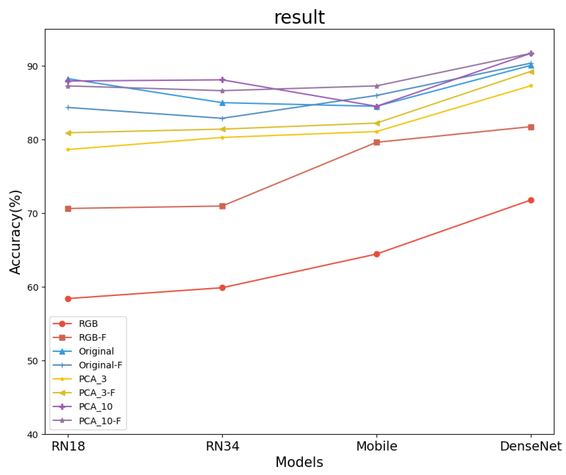
Given the challenges associated with collecting hyperspectral data and ensuring equitable data acquisition, we opted to pre-train neural networks on the comprehensive ImageNet dataset, which contains over 14 million labeled images across more than 20,000 categories, while maintaining consistent training parameters. This pre-training approach is widely recognized for enhancing accuracy and is extensively utilized in prior research. As illustrated in Figure 6, we compare experimental results between networks with and without pre-training. Although pre-training on ImageNet improves classification accuracy for RGB data, it still underperforms compared to hyperspectral data across all networks. As shown in Table 1 and

Table 3. Comparison of Classification $Accuracy$ ($Acc.$), $Recall$ (multiplied by 100), $F1-Score$ (F1, multiplied by 100), and $Kappa$ Score ($\kappa$, multiplied by 100) among neural networks fine-tuned on ImageNet pre-trained weights using varied inputs: dimension-reduced PCA features. “PCA_i” represents the i-dimensional PCA feature. Model abbreviations: RN18 (ResNet18), RN34 (ResNet34), MobileV2 (MobilenetV2), and Dense (Densenet121). Color convention: best and second best.

		RGB	Original	PCA_3	PCA_10
RN18	$Acc,$. (%)	70.63	84.34	80.91	87.27
	$\kappa$	69.42	83.71	80.13	86.75
	Recall	69.06	83.08	78.84	85.74
	F1	68.82	82.70	79.04	85.72
RN34	$Acc,$. (%)	70.96	82.87	81.40	86.62
	$\kappa$	69.77	82.18	80.62	86.08
	Recall	69.87	82.23	79.49	85.16
	F1	69.70	81.73	79.78	85.18
MobileV2	$Acc,$. (%)	79.61	85.97	82.22	87.27
	$\kappa$	78.78	85.40	81.49	86.75
	Recall	77.52	84.69	80.33	85.88
	F1	77.76	84.64	80.64	86.37
Dense	$Acc,$. (%)	81.73	90.53	89.23	91.68
	$\kappa$	80.98	90.15	88.79	91.34
	Recall	80.83	88.68	87.98	90.68
	F1	81.32	88.87	88.20	90.85

, DenseNet121 achieves the highest RGB data accuracy of 81.73% after ImageNet pre-training. In contrast, unprocessed hyperspectral data without pre-training reach an accuracy of 90.05%, marking an 8.32% increase, which represents a substantial gap in classification performance. Additionally, some hyperspectral-based networks exhibit decreased performance when pre-trained on ImageNet, likely due to the spatial distribution discrepancies between RGB and higher-dimensional data. This mismatch suggests the need for alternative technical adaptations. However, reducing data to three-dimensional PCA, closely resembling RGB data, slightly enhances performance in certain networks.

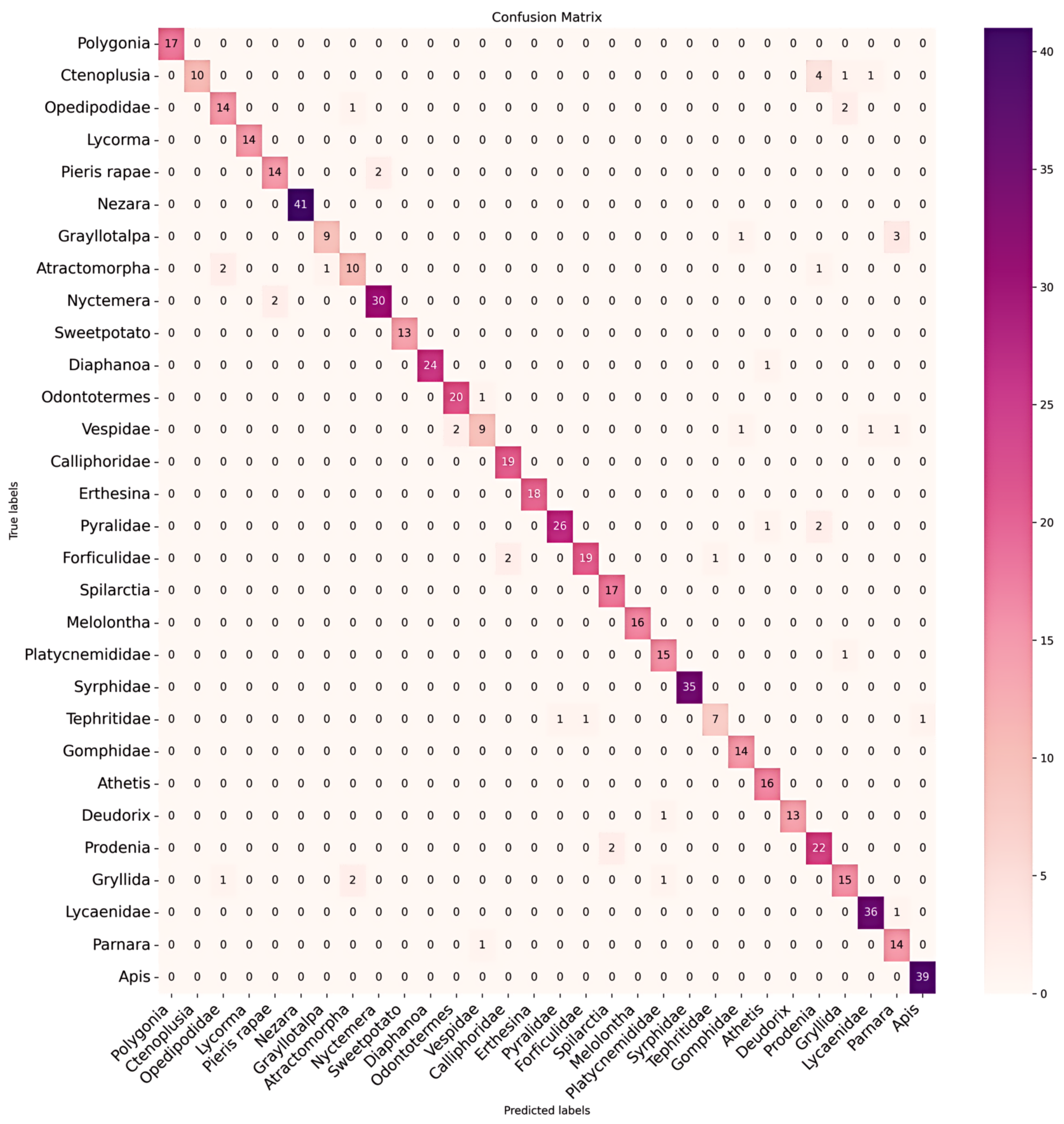
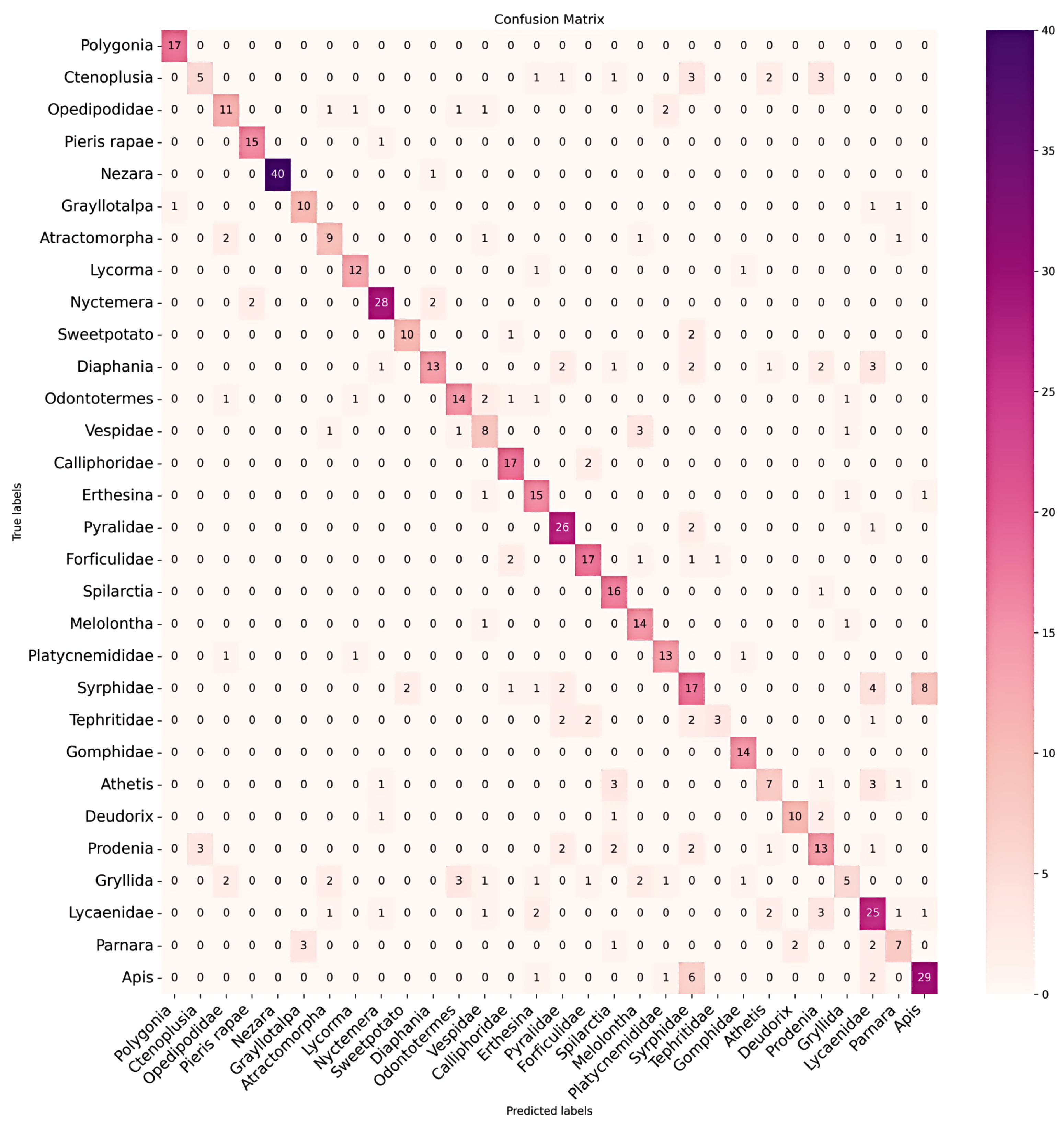
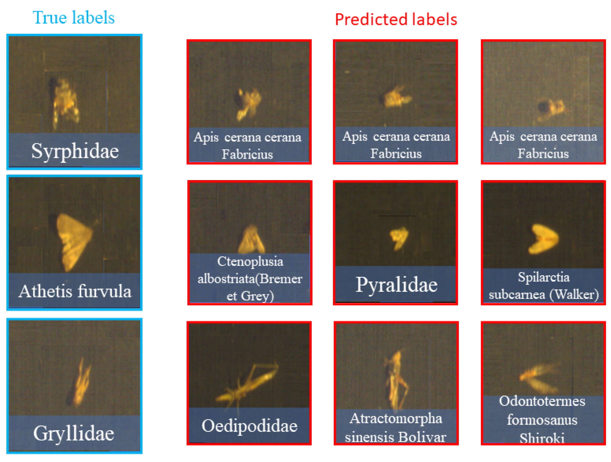
The confusion matrix diagrams in Figure 7 and Figure 8 provide a detailed comparison of classification between original hyperspectral and RGB data. They highlight the differences in true and predicted categories, emphasizing the superior classification accuracy of hyperspectral data. This advantage is particularly evident in categories where RGB data struggle due to morphological resemblances or taxonomic similarities among species. As seen in Figure 8, Syrphidae is incorrectly identified as Apis cerana cerana Fabricius, and similar errors occur with other species like Athetis fulvula and Prodenia litura (Fabricius). Notably, RGB data also confuse Grylidae for species with transparent wings and slender bodies, such as Oedipodidae, Atratomorpha sinensis Bolivar, and Vespidae (see Figure 9). Therefore, this underscores RGB’s limitations in accurately classifying related species and validates the superior efficacy of hyperspectral data in such classifications.

The noteworthy observation is that, with the hyperspectral channels reduced to three, equating to the same memory footprint as RGB data, the achieved results surpass those obtained with RGB data. We believe the regime behind the improvement is that the axes PCA provides are more canonical aligned. Among the various methods we tested, the most naive one was the traditional “sift + SVM” approach, only obtaining 28.06% accuracy. This is significantly lower compared to the other two manually extracted feature methods. While the histogram-based algorithm performs close to deep learning in terms of feature extraction and classification performance, overall, manual feature extraction methods fall short of the effectiveness achieved by deep learning-based ones. We further operated on hyperspectral data in Table 1, in three different settings for the input channel: the untouched original data preserving all channels, three PCA-ed channels, and ten PCA-ed channels. More channels were tested, showing no noticeable difference. It is obvious that shrinking the original data to a 3-PCA-ed channel format yields superior classification accuracy compared to RGB opponents across various metrics. However, the performance notably deteriorates when compared to the full-spectrum original data. This gap is particularly pronounced when utilizing the ResNet neural network architecture. In this context, the method with three PCA-ed channels reports a significant performance drop, which is over a 10 percent reduction in accuracy. This could be due to the loss of information when reducing from 128 channels to 3 channels. Furthermore, with 10 PCA-ed channels, better results were achieved compared to the full-spectrum original data. This indicates that the shrunken data exhibit a “denoising” effect, effectively disregarding the noise present in the full hyperspectral input and accelerating the entire inference process.

A $Recall$ score higher than the $F1-Score$ signifies the model’s strength in detecting positive instances while potentially conceding lower precision. This gap may be attributable to the model’s predisposition to designate more cases as positive—a factor that inflates $Recall$ but conversely amplifies the instances misclassified as positive. As observed in

Table 4. Comparison of classification $Recall$ (multiplied by 100), $F1-Score$ ($F1$, multiplied by 100) among different methods on varying inputs: rendered RGB, the original spectral data, and dimension-reduced PCA feature. “PCA_i” refers to the i-dimension PCA feature. Model abbreviations: RN18 (ResNet18), RN34 (ResNet34), MobileV2 (MobilenetV2), and Dense (Densenet121). A dash — means “not availiable”. Color convention: best, 2nd-best.

	Classifiers	RGB		Original		PCA_3		PCA_10		TBSCN
		$\mathit{Recall}$	$\mathit{F}\mathbf{1}$	$\mathit{Recall}$	$\mathit{F}\mathbf{1}$	$\mathit{Recall}$	$\mathit{F}\mathbf{1}$	$\mathit{Recall}$	$\mathit{F}\mathbf{1}$	$\mathit{Recall}$	$\mathit{F}\mathbf{1}$
DL	RN18	55.67	55.25	86.15	85.59	77.08	78.00	86.00	86.00	88.26	88.24
	RN34	58.41	59.05	86.27	82.74	78.00	78.20	86.34	86.31	87.6	87.76
	MobileV2	63.41	63.80	83.82	83.55	80.15	79.96	81.74	82.12	87.79	87.76
	Dense121	70.66	70.01	88.61	88.47	86.84	86.72	89.89	90.13	93.12	92.91
DL + SVM	RN18 + SVM	55.93	55.72	87.09	87.23	88.48	89.13	88.57	88.53	87.97	87.92
	RN34 + SVM	56.75	57.73	84.28	84.35	86.33	86.68	86.59	86.35	90.74	90.60
	Mobile + SVM	61.32	60.86	84.03	84.17	80.43	80.96	85.12	85.08	88.14	88.06
	Dense + SVM	70.86	69.44	89.27	89.38	86.02	85.99	91.22	91.23	91.25	91.96
HandScraft + SVM	Gabor + SVM	40.43	43.28	__	__	50.17	52.37	__	__	__	__
	SIFT + SVM	24.70	23.88	__	__	28.51	28.40	__	__	__	__
	Histogram + SVM	55.68	54.51	__	__	70.14	69.72	__	__	__	__

, $Recall$ slightly overshadows the $F1-Score$ in the original data’s classification results across a range of methods. Especially with the ResNet34 classifier, $Recall$ peaks at 86.27, while $F1$ lags at 82.74.

However, following PCA, the divergence between both metrics grows smaller regardless of channel number.With TBSCN, $Recall$, and $F1-Score$ are both enhanced, and their respective values converge, suggesting that the model successfully obtains a high positive class detection rate while avoiding classification error. We can obtain more information from Figure 10, which illustrates the UMAP [45] visualization of feature-extracted data from DenseNet, comparing RGB and hyperspectral datasets. Notably, RGB data points exhibit a higher degree of scatter and lack cohesive aggregation, unlike the hyperspectral data. This disparity is particularly evident when comparing with hyperspectral data reduced to three dimensions using PCA, which, despite matching the dimensional volume of RGB data, demonstrates superior clustering efficiency. However, while the PCA-reduced (10 dimensions) hyperspectral data show promising results, their UMAP representation reveals an excessive stacking of data points, leading to blurred inter-class boundaries. This effect suggests a potential overemphasis on data similarities due to the reduction to ten dimensions, possibly hindering feature extraction. Nevertheless, the application of TBSCN mitigates this issue, likely by optimizing the redundant information inherent in the 10-dimensional PCA data.

Accordingly, this procedure refines the model’s training quality, thereby boosting its ability to accurately recognize positive instances.

A study on different deep neural net backbones is given, where DenseNet [41] leads the leaderboard no matter how many channels are given and which input format is set. ResNet ranks the second. Fewer input channels will make accuracy more dependent on the classification network. On ResNet, the performance of RGB and PCA_3 differs significantly from DenseNet. It is also viable to combine deep net (as feature extractor) and SVM (as classifier), performing slightly less accurately than pure deep solution while over-performing handcraft features.

3.3. Further Analysis

This section prevents several ablation studies to the work. All experiment adopt the PCA_10 setting without training, using the PCA_10 classification results as the baseline. Figure 11 illustrates the distinctions observed in the ablation study.

3.3.1. Ablation Study on Random Correlation Section

In order to validate the effectiveness of the spectral and spatial correlation modules, separate experiments are conducted for each type of correlation, as seen in

Table 5. Comparison of Classification $Accuracy$ (Acc), $Recall$ (multiplied by 100), $F1-Score$ ($F1$, multiplied by 100), and $Kappa$ score ($\kappa$, multiplied by 100) among different methods on varied inputs: dimension-reduced PCA features. “PCA_i” represents the i-dimensional PCA feature. “Only spatial” denotes the exclusive focus on the two-branch structure, disregarding spectral information and concentrating solely on spatial information. Model abbreviations: RN18 (ResNet18), RN34 (ResNet34), MobileV2 (MobilenetV2), and Dense (Densenet121). Conversely, “Only spectral” refers to the exclusive attention to spectral information, neglecting spatial aspects. Color convention: best, 2nd-best.

		RN18	RN34	MobileV2	Dense	RN18 + SVM	RN34 + SVM	MobileV2 + SVM	Dense + SVM
PCA_10	Acc. (%)	87.93	88.09	84.50	91.68	90.54	87.92	86.30	92.50
	$Recall$	86.00	86.34	81.74	89.89	88.57	86.59	85.12	91.22
	$F1$	86.00	86.31	82.12	90.13	88.53	86.35	85.08	91.23
	$\kappa$	87.44	87.06	83.87	91.34	90.15	87.44	85.74	92.19
only spatial	Acc. (%)	89.55	90.05	87.27	92.82	91.68	91.03	90.05	93.64
	$Recall$	87.43	88.30	84.89	90.89	90.38	89.59	89.05	92.32
	$F1$	87.97	88.50	85.60	91.13	90.23	89.57	88.92	92.29
	$\kappa$	89.13	89.64	86.75	92.53	91.34	90.66	89.65	93.38
only spectral	Acc. (%)	88.42	88.90	87.11	93.31	91.57	89.72	89.56	93.96
	$Recall$	86.20	87.08	86.40	92.32	90.19	88.50	88.22	92.97
	$F1$	86.00	87.20	86.31	92.50	90.00	88.51	88.39	92.68
	$\kappa$	87.95	88.45	86.59	93.04	91.17	89.30	89.13	93.72
TBSCN	Acc. (%)	89.72	89.23	88.74	93.96	89.39	91.57	89.23	92.49
	$Recall$	88.26	87.60	87.79	93.12	87.97	90.74	88.14	91.25
	$F1$	88.24	87.76	87.76	92.91	87.92	90.60	88.06	90.96
	$\kappa$	89.30	88.79	88.29	93.72	88.97	91.18	88.80	92.19

. In the experiment where the spectral correlation was removed, the results for almost all deep learning-based classifiers were found to be inferior to those with the spectral correlation included. Similarly, when compared to scenarios where both spectral and spatial correlations were combined, experiments focusing solely on the spatial level produced lower results. It is worth noting that in experiments exclusively involving spectral correlation on the DenseNet architecture, results surpassed those involving only spatial correlation. Notably, the integration of both types of information resulted in a significant improvement in the results, particularly in comparison to other network architectures.

3.3.2. Ablation on Fusion Way

Experiments were conducted to explore the fusion of spatial and spectral information using two additional fusion methods: element-wise addition and element-wise multiplication. Importantly, when the two types of information were added together, the results were generally even less favorable than when centering exclusively on one type of information.

This suggests that spatial and spectral information represent distinct perspectives, and their additive combination can paradoxically deteriorate data enhancement. However, when the two types of information were multiplied element-wise, it yielded promising results. In a few instances, networks were able to perform well with this fusion approach, which involved concatenating both types of information and subsequently applying PCA for dimensionality reduction. As seen in

Table 6. Comparison of Classification $Accuracy$ (Acc), $Recall$ (multiplied by 100), $F1-Score$ ($F1$, multiplied by 100), and $Kappa$ score ($\kappa$, multiplied by 100) results among different methods. Model abbreviations: RN18 (ResNet18), RN34 (ResNet34), MobileV2 (MobilenetV2), and Dense (Densenet121). “s × s” denotes dot multiplication for integration for two-branch structures, while “s + s” signifies summation two information types. “ss_i” denotes information fusion downscaled to i dimensions by PCA. Color convention: best, 2nd-best.

		RN18	RN34	MobileV2	Dense	RN18 + SVM	RN34 + SVM	MobileV2 + SVM	Dense + SVM
s + s	Acc	88.41	90.86	86.62	91.68	91.35	91.03	88.58	92.98
	$Recall$	86.99	89.42	89.44	90.00	89.87	89.42	87.12	92.27
	$F1$	86.70	89.44	84.81	90.14	89.88	89.56	87.05	92.07
	$\kappa$	87.95	90.49	86.08	91.34	91.00	90.66	88.12	92.70
s × s	Acc	90.21	87.76	86.95	93.15	91.19	87.93	88.74	91.68
	$Recall$	89.10	86.04	85.74	92.32	90.06	85.71	87.48	90.37
	$F1$	88.90	86.17	85.70	92.14	89.99	85.99	87.57	90.13
	$\kappa$	89.82	87.77	86.42	92.87	90.83	87.43	88.29	91.34
ss_15	Acc	88.79	87.93	86.79	92.99	91.35	89.56	87.60	93.15
	$Recall$	87.10	86.24	85.00	91.83	89.50	88.93	85.96	92.16
	$F1$	87.29	86.32	84.80	91.88	89.66	88.54	85.87	92.05
	$\kappa$	88.80	87.44	86.25	92.70	91.00	89.14	87.10	92.87
ss_5	Acc	87.77	88.74	88.91	92.82	90.86	89.72	88.91	93.31
	$Recall$	85.56	87.24	87.27	91.67	89.26	88.12	87.77	92.44
	$F1$	86.09	87.14	87.14	91.71	89.28	87.87	87.55	92.39
	$\kappa$	87.26	88.29	88.46	92.53	90.49	89.30	88.46	93.04

.

3.3.3. Ablation Study on Input Channel

The study concludes with the selection of channel numbers, noting that the fusion approach, akin to TBSCN, involves concatenation followed by dimensionality reduction. Post-dimensionality reduction, when reducing the number of channels to 5 and 15, both outcomes surpassed the baseline results, but they exhibited a certain degree of decline compared to the scenario where dimensionality was reduced to 10 channels.

It is observed that, regardless of reducing dimensions to 5, 10, or 15, this fusion approach outperforms the “s + s” which means direct element-wise addition of the two types of information. While certain networks, such as ResNet18, may exhibit slightly better results in the classification of “s × s” scenarios, overall, concatenating the two types of information followed by dimensionality reduction is more operationally convenient and yields effective results. As seen in Table 6.

4. Conclusions

The recognition of insects plays a crucial role in a wide range of practical applications, such as agriculture, biodiversity conservation, and environmental monitoring. However, the inherent hyperspectral characteristics of insects often render them indistinguishable to the human eye in an RGB-dominated environment, highlighting the importance of insect recognition from a practical standpoint. Advancements in deep learning have significantly propelled the field of insect identification, highlighting the importance of high-quality data to support data-driven deep learning methods in this domain. While many studies have achieved commendable results in insect recognition, they predominantly focus on RGB data and overlook the significant role of spectral information. HI30 dataset fills this gap, comprising 30 categories and 2115 samples, thereby facilitating comprehensive research into hyperspectral insect classification. Experimental results strongly affirm the effectiveness of hyperspectral data in insect classification, outperforming RGB data. TBSCN model exploits the spatial and spectral dimensions of hyperspectral data through random spatial correlation and spectral correlation, thereby enhancing classification accuracy.

In future work, we will focus on expanding the exploration of hyperspectral data use in insect classification and enhancing our dataset. This initiative includes investigating the application of hyperspectral data in categorizing distinct insect subspecies, poised to make significant contributions to the realm of fine-grained classification tasks in this field.

References

- Stork, N.E.; McBroom, J.; Gely, C.; Hamilton, A.J. New approaches narrow global species estimates for beetles, insects, and terrestrial arthropods. Proc. Natl. Acad. Sci. USA 2015, 112, 7519–7523. [Google Scholar] [CrossRef] [PubMed]
- Majeed, W.; Khawaja, M.; Rana, N.; de Azevedo Koch, E.B.; Naseem, R.; Nargis, S. Evaluation of insect diversity and prospects for pest management in agriculture. Int. J. Trop. Insect Sci. 2022, 42, 2249–2258. [Google Scholar] [CrossRef]
- Wen, C.; Guyer, D. Image-based orchard insect automated identification and classification method. Comput. Electron. Agric. 2012, 89, 110–115. [Google Scholar] [CrossRef]
- Zhang, T.; Long, C.F.; Deng, Y.J.; Wang, W.Y.; Tan, S.Q.; Li, H.C. Low-rank preserving embedding regression for robust image feature extraction. IET Comput. Vis. 2023, 18, 124–140. [Google Scholar] [CrossRef]
- Deng, L.; Wang, Y.; Han, Z.; Yu, R. Research on insect pest image detection and recognition based on bio-inspired methods. Biosyst. Eng. 2018, 169, 139–148. [Google Scholar] [CrossRef]
- Alfarisy, A.A.; Chen, Q.; Guo, M. Deep Learning Based Classification for Paddy Pests & Diseases Recognition. In Proceedings of the 2018 International Conference on Mathematics and Artificial Intelligence, ICMAI ‘18, New York, NY, USA, 9–15 July 2018; pp. 21–25. [Google Scholar] [CrossRef]
- Wu, X.; Zhan, C.; Lai, Y.K.; Cheng, M.M.; Yang, J. IP102: A Large-Scale Benchmark Dataset for Insect Pest Recognition. In Proceedings of the 2019 IEEE/CVF Conference on Computer Vision and Pattern Recognition (CVPR), Long Beach, CA, USA, 15–20 June 2019; pp. 8779–8788. [Google Scholar] [CrossRef]
- Li, Y.; Wang, H.; Dang, L.M.; Sadeghi-Niaraki, A.; Moon, H. Crop pest recognition in natural scenes using convolutional neural networks. Comput. Electron. Agric. 2020, 169, 105174. [Google Scholar] [CrossRef]
- Abeywardhana, D.L.; Dangalle, C.D.; Nugaliyadde, A.; Mallawarachchi, Y. An ultra-specific image dataset for automated insect identification. Multimed. Tools Appl. 2022, 81, 3223–3251. [Google Scholar] [CrossRef]
- Hansen, O.L.; Svenning, J.C.; Olsen, K.; Dupont, S.; Garner, B.H.; Iosifidis, A.; Price, B.W.; Høye, T.T. Species-level image classification with convolutional neural network enables insect identification from habitus images. Ecol. Evol. 2020, 10, 737–747. [Google Scholar] [CrossRef] [PubMed]
- Kusrini, K.; Suputa, S.; Setyanto, A.; Agastya, I.M.A.; Priantoro, H.; Chandramouli, K.; Izquierdo, E. Data augmentation for automated pest classification in Mango farms. Comput. Electron. Agric. 2020, 179, 105842. [Google Scholar] [CrossRef]
- Wang, J.; Li, Y.; Feng, H.; Ren, L.; Du, X.; Wu, J. Common pests image recognition based on deep convolutional neural network. Comput. Electron. Agric. 2020, 179, 105834. [Google Scholar] [CrossRef]
- Zhang, L.; Zhao, C.; Feng, Y.; Li, D. Pests Identification of IP102 by YOLOv5 Embedded with the Novel Lightweight Module. Agronomy 2023, 13, 1583. [Google Scholar] [CrossRef]
- Li, W.; Zhu, T.; Li, X.; Dong, J.; Liu, J. Recommending advanced deep learning models for efficient insect pest detection. Agriculture 2022, 12, 1065. [Google Scholar] [CrossRef]
- De Backer, S.; Kempeneers, P.; Debruyn, W.; Scheunders, P. A band selection technique for spectral classification. IEEE Geosci. Remote Sens. Lett. 2005, 2, 319–323. [Google Scholar] [CrossRef]
- Kuo, B.C.; Li, C.H.; Yang, J.M. Kernel nonparametric weighted feature extraction for hyperspectral image classification. IEEE Trans. Geosci. Remote Sens. 2009, 47, 1139–1155. [Google Scholar]
- Huang, X.; Liu, X.; Zhang, L. A Multichannel Gray Level Co-Occurrence Matrix for Multi/Hyperspectral Image Texture Representation. Remote Sens. 2014, 6, 8424–8445. [Google Scholar] [CrossRef]
- Shen, L.; Jia, S. Three-dimensional Gabor wavelets for pixel-based hyperspectral imagery classification. IEEE Trans. Geosci. Remote Sens. 2011, 49, 5039–5046. [Google Scholar] [CrossRef]
- Deng, Y.J.; Li, H.C.; Tan, S.Q.; Hou, J.; Du, Q.; Plaza, A. t-Linear Tensor Subspace Learning for Robust Feature Extraction of Hyperspectral Images. IEEE Trans. Geosci. Remote Sens. 2023, 61, 5501015. [Google Scholar] [CrossRef]
- Deng, Y.J.; Yang, M.L.; Li, H.C.; Long, C.F.; Fang, K.; Du, Q. Feature Dimensionality Reduction with L 2, p-Norm-Based Robust Embedding Regression for Classification of Hyperspectral Images. IEEE Trans. Geosci. Remote Sens. 2024, 62, 5509314. [Google Scholar] [CrossRef]
- Tarabalka, Y.; Fauvel, M.; Chanussot, J.; Benediktsson, J.A. SVM-and MRF-based method for accurate classification of hyperspectral images. IEEE Geosci. Remote Sens. Lett. 2010, 7, 736–740. [Google Scholar] [CrossRef]
- Huang, K.; Li, S.; Kang, X.; Fang, L. Spectral–spatial hyperspectral image classification based on KNN. Sens. Imaging 2016, 17, 1. [Google Scholar] [CrossRef]
- Xia, J.; Ghamisi, P.; Yokoya, N.; Iwasaki, A. Random forest ensembles and extended multiextinction profiles for hyperspectral image classification. IEEE Trans. Geosci. Remote Sens. 2017, 56, 202–216. [Google Scholar] [CrossRef]
- Khodadadzadeh, M.; Li, J.; Plaza, A.; Bioucas-Dias, J.M. A subspace-based multinomial logistic regression for hyperspectral image classification. IEEE Geosci. Remote Sens. Lett. 2014, 11, 2105–2109. [Google Scholar] [CrossRef]
- Chen, Y.; Lin, Z.; Zhao, X.; Wang, G.; Gu, Y. Deep learning-based classification of hyperspectral data. IEEE J. Sel. Top. Appl. Earth Obs. Remote Sens. 2014, 7, 2094–2107. [Google Scholar] [CrossRef]
- Chen, Y.; Zhao, X.; Jia, X. Spectral–spatial classification of hyperspectral data based on deep belief network. IEEE J. Sel. Top. Appl. Earth Obs. Remote Sens. 2015, 8, 2381–2392. [Google Scholar] [CrossRef]
- Ge, Z.; Cao, G.; Li, X.; Fu, P. Hyperspectral Image Classification Method Based on 2D–3D CNN and Multibranch Feature Fusion. IEEE J. Sel. Top. Appl. Earth Obs. Remote Sens. 2020, 13, 5776–5788. [Google Scholar] [CrossRef]
- Wu, H.; Li, D.; Wang, Y.; Li, X.; Kong, F.; Wang, Q. Hyperspectral Image Classification Based on Two-Branch Spectral–Spatial-Feature Attention Network. Remote Sens. 2021, 13, 4262. [Google Scholar] [CrossRef]
- Jin, H.; Peng, J.; Bi, R.; Tian, H.; Zhu, H.; Ding, H. Comparing Laboratory and Satellite Hyperspectral Predictions of Soil Organic Carbon in Farmland. Agronomy 2024, 14, 175. [Google Scholar] [CrossRef]
- Carrino, T.A.; Crósta, A.P.; Toledo, C.L.B.; Silva, A.M. Hyperspectral remote sensing applied to mineral exploration in southern Peru: A multiple data integration approach in the Chapi Chiara gold prospect. Int. J. Appl. Earth Obs. Geoinf. 2018, 64, 287–300. [Google Scholar] [CrossRef]
- Shao, Y.; Ji, S.; Xuan, G.; Ren, Y.; Feng, W.; Jia, H.; Wang, Q.; He, S. Detection and Analysis of Chili Pepper Root Rot by Hyperspectral Imaging Technology. Agronomy 2024, 14, 226. [Google Scholar] [CrossRef]
- Long, C.F.; Wen, Z.D.; Deng, Y.J.; Hu, T.; Liu, J.L.; Zhu, X.H. Locality Preserved Selective Projection Learning for Rice Variety Identification Based on Leaf Hyperspectral Characteristics. Agronomy 2023, 13, 2401. [Google Scholar] [CrossRef]
- Xiao, Z.; Yin, K.; Geng, L.; Wu, J.; Zhang, F.; Liu, Y. Pest identification via hyperspectral image and deep learning. Signal Image Video Process. 2022, 16, 873–880. [Google Scholar] [CrossRef]
- Zheng, Y.; Zhang, T.; Fu, Y. A large-scale hyperspectral dataset for flower classification. Knowl.-Based Syst. 2022, 236, 107647. [Google Scholar] [CrossRef]
- Xu, Y.; Du, B.; Zhang, F.; Zhang, L. Hyperspectral image classification via a random patches network. ISPRS J. Photogramm. Remote Sens. 2018, 142, 344–357. [Google Scholar] [CrossRef]
- Cheng, C.; Li, H.; Peng, J.; Cui, W.; Zhang, L. Hyperspectral image classification via spectral-spatial random patches network. IEEE J. Sel. Top. Appl. Earth Obs. Remote Sens. 2021, 14, 4753–4764. [Google Scholar] [CrossRef]
- Shenming, Q.; Xiang, L.; Zhihua, G. A new hyperspectral image classification method based on spatial-spectral features. Sci. Rep. 2022, 12, 1541. [Google Scholar] [CrossRef] [PubMed]
- Deng, J.; Dong, W.; Socher, R.; Li, L.J.; Li, K.; Fei-Fei, L. Imagenet: A large-scale hierarchical image database. In Proceedings of the 2009 IEEE Conference on Computer Vision and Pattern Recognition, Miami, FL, USA, 20–25 June 2009; pp. 248–255. [Google Scholar]
- Zapryanov, G.; Ivanova, D.; Nikolova, I. Automatic White Balance Algorithms forDigital StillCameras—A Comparative Study. Inf. Technol. Control. 2012. Available online: http://acad.bg/rismim/itc/sub/archiv/Paper3_1_2012.pdf (accessed on 8 March 2024).
- He, K.; Zhang, X.; Ren, S.; Sun, J. Deep residual learning for image recognition. In Proceedings of the IEEE Conference on Computer Vision and Pattern Recognition, Las Vegas, NV, USA, 27–30 June 2016; pp. 770–778. [Google Scholar]
- Huang, G.; Liu, Z.; Van Der Maaten, L.; Weinberger, K.Q. Densely connected convolutional networks. In Proceedings of the IEEE Conference on Computer Vision and Pattern Recognition, Honolulu, HI, USA, 21–26 July 2017; pp. 4700–4708. [Google Scholar]
- Sandler, M.; Howard, A.; Zhu, M.; Zhmoginov, A.; Chen, L.C. Mobilenetv2: Inverted residuals and linear bottlenecks. In Proceedings of the IEEE Conference on Computer Vision and Pattern Recognition, Salt Lake City, UT, USA, 18–23 June 2018; pp. 4510–4520. [Google Scholar]
- Magnusson, M.; Sigurdsson, J.; Armansson, S.E.; Ulfarsson, M.O.; Deborah, H.; Sveinsson, J.R. Creating RGB images from hyperspectral images using a color matching function. In Proceedings of the IGARSS 2020—2020 IEEE International Geoscience and Remote Sensing Symposium, Waikoloa, HI, USA, 26 September–2 October 2020; pp. 2045–2048. [Google Scholar]
- Pedregosa, F.; Varoquaux, G.; Gramfort, A.; Michel, V.; Thirion, B.; Grisel, O.; Blondel, M.; Prettenhofer, P.; Weiss, R.; Dubourg, V.; et al. Scikit-learn: Machine Learning in Python. J. Mach. Learn. Res. 2011, 12, 2825–2830. [Google Scholar]
- McInnes, L.; Healy, J.; Melville, J. Umap: Uniform manifold approximation and projection for dimension reduction. arXiv 2018, arXiv:1802.03426. [Google Scholar]
Figure 1.
A sample in the HI30 dataset comprises 3D data, with H and W denoting the height and width of the image, respectively, while B represents the spectral dimension of the data.
Figure 2.
Schematic of hyperspectral imaging system.
Figure 3.
Taxonomy of the HI30 dataset. Displaying only a portion of the genera and species within the dataset as a taxonomic representation, with more comprehensive information available in the appendices.
Figure 4.
The feature extractor proposed for tackling spectral pest classification. Starting with the original spectral input, two net branches featuring random spatial correlation and random spectral correlation are used for extracting features from different prospective. For the random spatial correlation, patches are selected randomly, serving as convolutional kernel weights, resulting in feature maps after convolution (denoted as ⊗ in the figure). This is repeated L times. For the random spectral correlation, patches are selected and averaged along the spatial dimensions, saved as kernels, resulting in feature maps after convolution. Two kinds of feature maps are fused and compressed using PCA, then combined with the original spectral input to feed the classifier.
Figure 5.
Visualization of top 10 PCA channels of the selected HI30 samples. The Viridis colormap is used for color encoding. The first column is rendered RGB data. a,b,c,d, respectively, represent Pieris rapae, Gryllidae, Nyctemera adversata Walker, and Melolontha.
Figure 6.
Comparison of classification accuracy among neural network architectures using varied inputs: “PCA_i” denotes the i-dimensional PCA feature, and “-F” indicates fine-tuning on ImageNet pre-trained weights. Model abbreviations: RN18 (ResNet18), RN34 (ResNet34), MobileV2 (MobilenetV2), and Dense (Densenet121).
Figure 7.
This confusion matrix illustrates the classification outcomes of original hyperspectral data using the DenseNet121 classification method. The vertical axis represents the true labels, while the horizontal axis indicates the predicted labels.
Figure 8.
This confusion matrix presents the classification results using RGB data and indicates the underperformance in certain categories compared to the original hyperspectral data. It employs the DenseNet121 classification method, with the vertical axis representing the true labels and the horizontal axis representing the predicted labels.
Figure 9.
The examples of misclassification derived from RGB data. Each row represents a unique category with correct label examples on the left column and misclassified samples on the right.
Figure 10.
2D UMAP feature visualization on different inputs. The feature used here are extracted from last layer of DenseNet121. More distributed for different color clusters, the better discriminative the feature is.
Figure 11.
Ablation studies are alongside baseline metrics. (a) compares results of spectral correlation and spatial correlation individually with the baseline. (b) illustrates the impact of different fusion method on spectral and spatial information. (c) demonstrates the comparison of the final input dimensions.