Genomic Selection in Cereal Breeding


1
Sejet Plant Breeding I/S, 8700 Horsens, Denmark
2
Center for Quantitative Genetics and Genomics, Aarhus University, 8830 Tjele, Denmark
*
Author to whom correspondence should be addressed.
Agronomy 2019, 9(2), 95; https://doi.org/10.3390/agronomy9020095
Submission received: 21 December 2018
/
Revised: 13 February 2019
/
Accepted: 14 February 2019
/
Published: 19 February 2019
(This article belongs to the Special Issue Molecular Genetics, Genomics and Biotechnology of Crop Plants Breeding)
Abstract
:Genomic Selection (GS) is a method in plant breeding to predict the genetic value of untested lines based on genome-wide marker data. The method has been widely explored with simulated data and also in real plant breeding programs. However, the optimal strategy and stage for implementation of GS in a plant-breeding program is still uncertain. The accuracy of GS has proven to be affected by the data used in the GS model, including size of the training population, relationships between individuals, marker density, and use of pedigree information. GS is commonly used to predict the additive genetic value of a line, whereas non-additive genetics are often disregarded. In this review, we provide a background knowledge on genomic prediction models used for GS and a view on important considerations concerning data used in these models. We compare within- and across-breeding cycle strategies for implementation of GS in cereal breeding and possibilities for using GS to select untested lines as parents. We further discuss the difference of estimating additive and non-additive genetic values and its usefulness to either select new parents, or new candidate varieties.
1. Introduction
Agronomically important quantitative traits are often controlled by many small-effect genes, which have been difficult to take advantage of in practical breeding [1]. The small-effect genes are difficult to map, and, if mapping is successful, often multiple quantitative trait loci (QTL) are present, which are difficult to use simultaneously in breeding. As a consequence, marker-assisted-selection (MAS), when defined as the use of mapped genes in breeding, has had limited success in improving such traits [2]. A key example quantitative trait is yield, which has shown difficult to improve in nearly all plant crops [3,4]. Gene editing, like CRISPR (Clustered Regularly Interspaced Short Palindromic Repeats), will likely not offer a solution either, because, like MAS, they are conditional on first identifying mutations or modifications with large effect. Genomic (or genome-wide) selection (GS) is a method that has promised to overcome the limitations of MAS for quantitative traits [2]. The objective of GS is to determine the genetic potential of an individual instead of identifying the specific QTL. GS was originally developed in livestock breeding as a method to predict breeding values of individuals based on markers covering the whole genome using simulated data [5]. Initial studies on the application of GS in a dairy cattle breeding program showed promising improvements in the accuracy of selection [6]. Promisingly, GS have been indicated to outperform MAS using the same economic investment, even at low accuracies [7,8]. It may be noted that before GS was established, plant breeders already developed ideas with similar ingredients as Meuwissen et al.’s GS [5]. Notably, Bernardo [9] developed a multi-marker MAS version with random marker effects, but it was developed within the MAS paradigm using only markers flanking identified QTL, while the main break-through in Meuwissen et al.’s GS [5] was to avoid identifying QTL.
Decreasing costs of genotyping using high-density single nucleotide polymorphism (SNP)-arrays and development of statistical methods to accurately predict marker effects have led to the breakthrough of GS. Selection decisions based on GS results have been indicated to improve the accuracy of selection and speed of genetic improvement. GS is now used in dairy cattle breeding programs around the world and included in the marketing of bulls [10]. Plant breeders have often been relying on phenotypic selection (PS) to choose the best offspring to continue in the breeding program. One of the first studies on the prospects of GS in plant breeding was carried out in maize (Zea mays L.) by Bernardo et. al [8] using simulated data. Predictions have also been carried out in cereals as wheat (Triticum aestivum L.) [11], barley (Hordeum vulgare L.) [12], and oat (Avena sativa L.) [13]. The potential of GS has been explored in both hybrid breeding [14,15] and inbred or double haploid (DH) lines [16], and in most cases authors conclude that prediction accuracies are sufficient to make GS more efficient than PS.
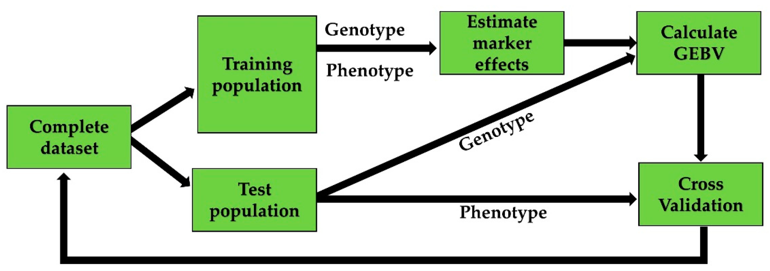
To capture the total genetic variance, the effect of each marker in the whole marker-set is estimated in GS regardless of the significance threshold, assuming that markers are in linkage disequilibrium (LD) with the QTLs. Marker effects are estimated using individuals with both genotypic and phenotypic information. The estimated marker effects are combined with marker information of an individual to give the genomic-estimated-breeding-value (GEBV). The predictive ability of the model is calculated based on a cross-validation (CV) system using a training- and a test-population to optimize the model. Marker effects are calculated based on genotypes and phenotypes from the training-population. Subsequently, GEBVs are estimated for the test-population based on these calculations. The predictive ability of the model is then calculated as the correlation between GEBV and phenotypes of the test-population (Figure 1).
Many papers have now established that GS is a promising approach in different plant species, and several reviews have considered the basic approaches of GS [2], and comparison of statistical methods for GS [17]. There is still limited attention for the ways that GS can fit in plant-breeding programs, how information would flow, the relevance of close and distant relationships in GS implementation, and where to improve accuracy or speed of the program. It is currently a timely moment to review in more detail how GS could be used to improve plant-breeding systems. Most research on GS in plants has ignored pedigree-information, unlike animal GS applications, and it appears useful to discuss the use of pedigree in plants as well.
This review will explore features of GS set-up in cereal breeding, including size of training population, the relationship between individuals in the training and the test data, and marker density. The paper also includes a comparison of implementation strategies for GS in a breeding program, making predictions within and across breeding cycles, as well as the potential to select parents purely based on GEBV. We use breeding of cereals, like wheat and barley based on DH lines, as our primary example to describe GS in plant breeding, but most of our discussion will equally apply to breeding of other inbred and self-fertilizing species.
2. The Set-Up of Genomic Selection
This section describes in more detail the set-up of GS as shown in Figure 1, and factors affecting the accuracy of genomic predictions.
2.1. Size of Training Data
Several studies have shown that prediction accuracies are influenced by the training population size. It is highly important for breeders to determine the number of lines to be genotyped and phenotyped to establish a suitable training data set, because set-up of the first training data is often a large investment. In a study of spring-barley, Nielsen et al. [18] observed a reduced accuracy of GS as a result of reducing the training data set, and moreover, accuracies appeared less stable with CV rounds showing larger variation in accuracy for a small training data set. Cericola et al. [19] found an increase in prediction accuracy with increasing training population size, reaching a plateau at ~700 lines consisting of full-sib, half-sib, and less related wheat lines from 3 consecutive breeding cycles. However, the optimal training set size was found to be higher in a study by Norman et al. [20] using training set sizes varying from 250 to 8300 lines with differing relationships. An increase in prediction accuracy as a results of increased training population size was also observed by Meuwissen [21] using distantly related individuals.
2.2. Relatedness between Training and Test Individuals
The accuracy of GS models has been shown to be affected by the relatedness of individuals between the training and test population [22]. Isidro et al. [23] found the highest prediction accuracies when training data represented the whole population and had a strong relationship to the test data. Relatedness between individuals has also been a subject of interest in MAS. Gowda et al. found that the relatedness between individuals severely impacts QTL-estimation using MAS in hybrid-wheat [24]. Decreasing prediction accuracies for GS with less related individuals in the training and test population was also observed by Lorenz et al. [25], and Nielsen et al. [18] found a decrease in prediction accuracy when using less related individuals in a leave-family-out CV strategy.
2.3. Cross-Validation Strategies
To get an initial assessment of genomic prediction accuracies, most studies run a CV within the collected training data, as introduced for GS studies by Meuwissen et al. [5]. CV makes predictions for individuals, excluding their own phenotypes from the prediction model. The two main CV strategies are leave-one-out (LOO) and k-fold CV, where k-fold CV can be further subdivided as using random folds or stratified folds. In LOO, one line is left out and predicted based on the remaining population, which is repeated for every line as performed by Nielsen et al. [18]. In a random k-fold CV, the population is divided into a number (k) of random groups and one group is left out and predicted based on the remaining ones. In a stratified k-fold CV, grouping can be based on, for instance, families, breeding cycles, locations, environments, etc., and again one group is left out and predicted based on the remaining ones. Random and stratified k-fold CV strategies, where the stratified version was based on breeding cycles, have been carried out by Cericola et al. [19].
Each of the CV approaches will be relevant for a particular use in breeding. In LOO and random k-fold CV, the line(s) predicted typically have closely related individuals in the training data, as well as many samples from the same year, location, and environment as the ones left-out, and are available in the training set. This situation is relevant to test predictions for lines that have not been phenotyped for some trait, based on phenotypes from closely related material in the same breeding cycle. It can, for instance, apply to quality traits that are only measured on a subset to supply predictions for the lines without the quality trait measurements. In a stratified k-fold CV, situations can be tested, such as forward prediction from an older generation as training to a newer generation as test, or predictions across locations or across environments. Results from stratified k-fold CV can be relevant to test GS strategies that shorten the breeding cycle, or that reduce testing in locations and environments.
The effect of relationships on prediction accuracy can also be seen in CV, where LOO and random k-fold CV often show higher prediction accuracy than stratified k-fold CV [26]. The different levels of relationships between training and test data is one major factor to explain these differences, because LOO and random k-fold CV tend to have higher relationships between training and test individuals than the stratified k-fold CV strategies. Additionally, genotype by environment interaction (GxE) may contribute to poorer prediction accuracy when the stratification is across years or environments.
2.4. Marker Density
Several studies have investigated the possibility to use a reduced marker set for GS without affecting prediction accuracies remarkably. Using a smaller marker set would reduce the genotyping costs for each line in the training population, making it feasible to genotype more individuals for the same expense. Meuwissen [21] found that prediction accuracies are increasing with an increase in marker density. It can be argued that at least one marker should be in LD with each QTL to capture all the genetic variation in a population. This is especially the case for unrelated lines, as LD between markers may vary between the training and the test population. Using genetically related barley lines, Nielsen et al. [18] observed a remarkable decrease in prediction accuracy when using less than 1000 markers, however this was dependant on the trait. Cericola et. al [19] also concluded that using 1000 randomly selected and spaced markers was enough to reach maximum prediction accuracy in wheat breeding lines. High marker density has been observed to be more critical when predicting more distant relatives [20].
2.5. Prediction of Genomic Estimated Breeding Values (GEBV)
Estimation of breeding values by Best Linear Unbiased Prediction (BLUP) in a mixed model using a pedigree-based relationship matrix was already introduced in animal breeding for selection based on phenotypes and pedigree [27]. This pedigree-based BLUP serves as the basis of one of the most-popular practical approaches to estimate GEBV by using “genomic BLUP” (GBLUP). In GBLUP, the pedigree-matrix is replaced by a G-matrix representing the genomic relationship between individuals, as described by VanRaden et al. [28]. GBLUP is a mixed model, which in the most basic form can be written as:
where y is a vector of phenotypes, β is a vector of fixed-effects, α is a vector of genomic breeding values, X and Z are design matrices, and ε is a vector of residual effects. In the mixed model (1), genomic breeding values have the multivariate Normal distribution . GBLUP can directly provide GEBV for an individual without phenotypes by simply adding it in the G-matrix. Kernel-methods, similarly to GBLUP, apply similarity (or distance) matrices and are more versatile than GBLUP in that they also capture non-additive effects (see Text Box 1 for details).
Genomic prediction can also be based on models that estimate marker-effects for all genome-wide markers simultaneously. A basic model for this approach can be described as in (1), but where Z contains genotypes and α are the marker effects. Regression on markers from the whole genome will often face the problem of the number of markers being much larger than the number of observations, causing a lack of degrees of freedom when estimating the marker effects simultaneously with the least square method. The problem is also known as “large p – small n” and is often solved in GS by using a mixed model treating marker effects random to obtain BLUP of marker effects [5], or by one of many Bayesian regression models, known as the "Bayesian alphabet" (reviewed in [29] and described in more detail in Text Box 1). The difference between the BLUP of marker effects and the Bayesian regression models lies in the assumption about the distribution of marker-effects. BLUP assumes that marker effects follow a Normal distribution with an equal variance for all loci. In the Bayesian methods, heavy-tailed prior distributions or mixture distributions are used as the distribution of maker-effects (see Text Box 1 for details), allowing for some markers to contribute more to genomic variance than others. Bayesian methods often rely on using Markov-Chain Monte Carlo (MCMC) to estimate the model parameters.
The models for genomic prediction have been extensively compared. Meuwissen et al. [5] originally compared four different statistical methods for GS, least-square estimation (LS), BLUP, and two Bayesian estimation methods, BayesA and BayesB. In their study, BLUP outperformed LS remarkably having a correlation between estimated and true breeding values of 0.732 and 0.318, respectively. Additional increases in accuracies compared to GBLUP were observed for BayesA (~9%) and BayesB (~16%). More extensive comparisons of prediction models can be found in Heslot et al. [30], Maltecca et al. [31], and De Los Campos et al. [17], typically concluding that when predicting close relatives and considering a trait affected by many genes of small effect, differences between the methods are small, and methods like (G)BLUP and ridge regression are effective and robust; when traits have some larger QTL or when considering prediction of distant relatives, improvements in prediction accuracy can be obtained from Bayesian and machine learning methods, where in particular BayesB and BayesC(pi) are popular. In plant breeding, the kernel-methods are also popular, in particular to predict non-additive effects and to handle complex multi-environment multi-trait models [32,33]. Also, the popular “deep learning” or deep belief networks have been applied and compared recently, but performed poorer than existing genomic prediction methods [34]. For situations where Bayesian or machine-learning methods prove useful to improve prediction accuracy, but computational time for these methods prohibits fast routine use, Su et al. [35] introduced a weighted GBLUP (WGBLUP) using SNP-weights based on results from a Bayesian model.
Text Box 1. Statistical models for genomic prediction.
Mixed models estimating marker effects as “random regressions” by BLUP [5].
Bayesian Lasso [36] and Bayesian regression models from the “Bayesian alphabet” [29], such as BayesA and BayesB [5], BayesC, BayesCpi [37], and BayesR [38]. These are all multiple-regression models, like the mixed model, but with Bayesian shrinkage approaches applied to treat the marker-effects. Bayesian Lasso and BayesA apply non-differential shrinkage by applying a long-tail distribution to marker effects, being LaPlace and student-t, respectively. It has been recognized that the shrinkage in Bayesian Lasso and BayesA is still quite uniform [39], like the mixed model, which has led to variations when applying more extreme long-tailed distributions, such as the normal exponential gamma [40], the power-exponential distribution (Power Lasso, [41]), and the modifications proposed by Fang et al. [39]. The BayesB, BayesC(pi), and BayesR methods apply a mixture of distributions as the prior distribution of marker effects, one of which can be a spike at zero, and where BayesB and BayesC(pi) use two distributions, and BayesR uses four. Other Bayesian models applying mixture distributions fall in this same category, such as SSVS [42] and the methods based on George and McCulloch 's [43] Bayesian Variable Selection applied in Kapell et al. [44] and Gao et al. [41], the latter also using a four-mixture distribution as in BayesR.
Statistical and machine learning methods for high-dimensional data, such as support vector machines [45], ridge regression [46,47], and Bayesian additive regression trees [48].
Methods that do not estimate marker effects but collapse marker data into relationship or similarity or distance matrices, such as the mixed model GBLUP [28] and kernel methods [49,50]. In these methods, the kernel-methods can be seen as modifications and extensions of GBLUP by implicitly considering multiple and different relationship measures than only the additive relationships considered in GBLUP. The kernel-methods have been shown to also capturing epistatic and other non-additive relationships [51]. It is possible to also extend GBLUP in similar ways, i.e., by including a second relationship matrix, which is the Hadamard product of G, a mixed model is obtained that also captures (two-way) epistatic interactions [51,52].
3. Strategies for Implementation of Genomic Selection
3.1. Basic Breeding Scheme in Cereals
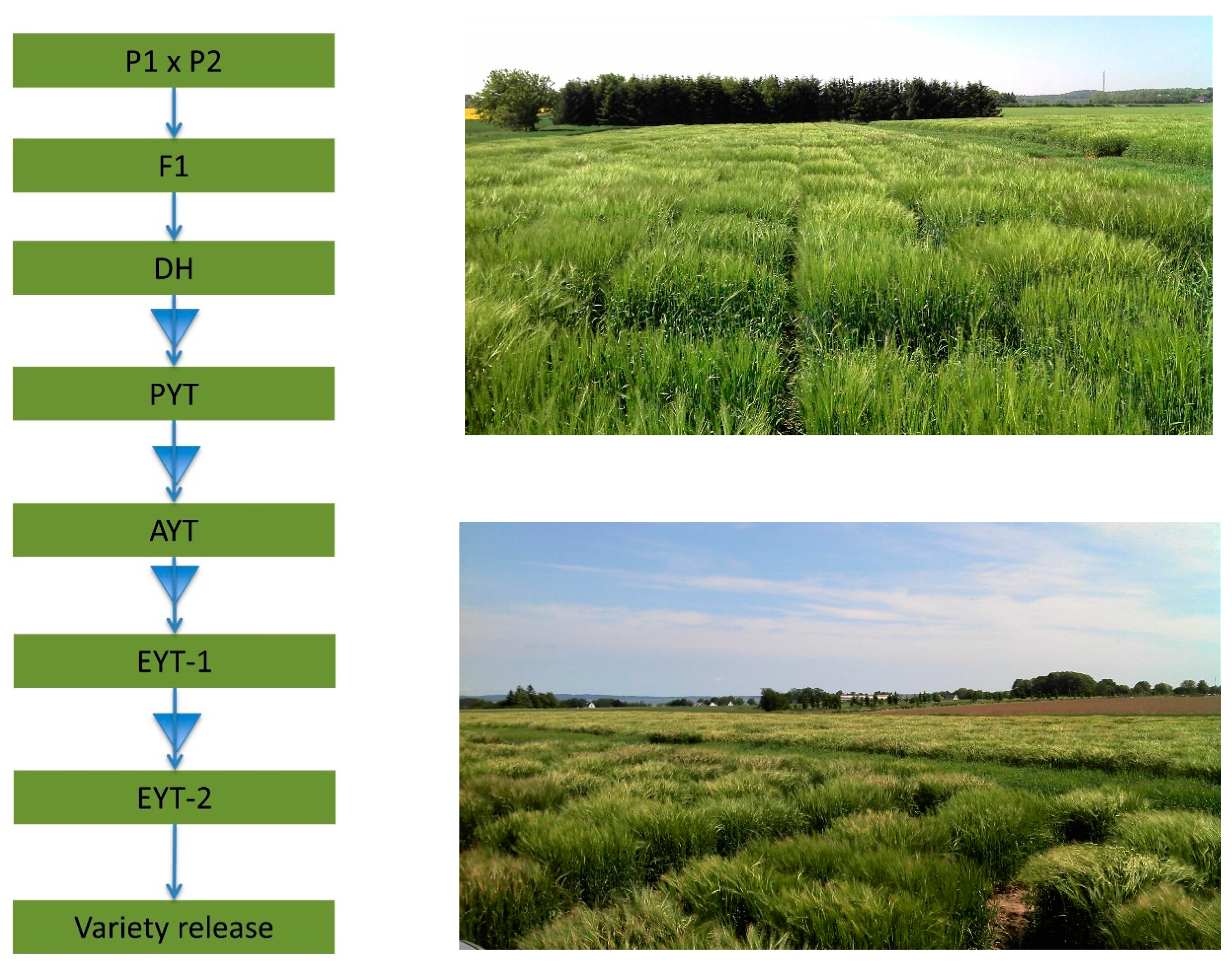
We will first describe an example of a standard barley breeding-scheme using double DHs, shown in Figure 2. In this standard breeding scheme, two parents are crossed to make an F1 progeny, and from pollen culture of the F1 a large set of fully inbred DH progeny can be developed. Every DH will have a unique mosaic of the parental genomes, and the main task of the breeder is to sort among the DH progeny to identify the ones with the best combination of parental alleles. However, agronomic traits, such as yield, cannot be determined on the single DH plants, and s seed of each DH is multiplied to allow sowing yield trials for each DH genotype. After the first multiplication step, there is enough seed to sow one small plot called Preliminary Yield Trial (PYT); after the second multiplication step, there is enough seed for about 3 replicates at 2 locations called Advanced Yield Trials (AYT). Since barley is a self-pollinating crop, the seed from harvested yield trials can be used to perform trials in multiple locations called Elite Yield Trial (EYT) in the following crop cycle. At each multiplication step, breeders will select and reduce the number of DH lines retained, because limited space and resources for field trials will not allow progressing all DH progeny to the final EYT stage. The optimal way to implement GS in plant breeding programs is not straightforward and multiple different strategies have been discussed in the literature [55,56].
3.2. Across-Breeding Cycle Genomic Selection
GS was first introduced with prediction across generations in animals, where marker effects are calculated on the basis of one generation and used for selection of individuals with an unknown phenotype in the upcoming generation [5]. The equivalent of this strategy in plant breeding would be to predict across breeding cycles. Improvement of genetic gains in animal breeding have mainly been due to selection of traits where phenotypes cannot be directly measured, such as sex-limited traits or traits related to meat-quality [57]. The analogy in plant breeding would be to improve selection in the early stages of the breeding program for traits that are difficult to measure with a low amount of seeds, such as yield and some quality parameters. For instance, malting quality in barley has been considered a good target for GS [58] and baking quality in wheat [59]. Figure 3 shows how data from PYT can be used for GS2 of DH-lines in the next generation. Subsequent selection steps, for instance from PYT to AYT, can similarly be based on data from the previous year. In these steps own data for each line also becomes available, reducing the need to rely on previous generations’ data to compute GEBV. Only a few studies have used phenotypic data from single plot PYT in GS models [60], while most GS studies have evaluated use of concluded 2-year EYT data as training data. As shown in Figure 3, there would be a 4-year lag when using concluded EYT data to make predictions on DH, and when using concluded EYT data in later selection steps, the lag would be more than 4 years.
As described before, most studies on GS in plant breeding have found that good prediction accuracies are only obtained when the training and test data are well related. Hence, an important requirement for the across-breeding cycle GS to work well, is that the relationships between subsequent years are high, i.e., there must be many of the same parents used in the crossings of subsequent years, or the crossings must be based on progeny of previous years that are re-used as parents. Often, varieties released by other breeders enter the breeding program to supply new genetic material, which could make it a challenge to keep the breeding material sufficiently related for across-breeding cycle GS to work well [61], and without modifications in the breeding program, there is a time-lag of 6 years for the use of own progeny as new parents. Using data from a real breeding program, Cericola et al. [19] observed low prediction accuracy between breeding cycles, which could indeed be attributed to low overlap of parents and low relationship between breeding cycles.
3.3. Within-Breeding Cycle Genomic Selection
Another way to implement GS is within the generations of one breeding cycle, as shown on Figure 2. Here, lines from the same breeding cycle are used as a training population for GS, for instance to predict sister-lines with missing phenotypes. This type of prediction of sister-lines can be optimized by purposely reducing phenotyping, or by omitting environments, or to measure expensive (quality) traits on only a part of the progeny and predict the rest. Additionally, GEBV combined with phenotypes will improve accuracy of line selection to continue in the breeding program, and with subsequent generation, new phenotypic information will become available for the individuals making GEBVs more accurate, thereby further assisting in the selection process. Predictions within a generation will often have a high relationship between lines as multiple lines from each family are tested. The accuracy of selection is increased with GS within generation, especially for early years where each line has a limited number of phenotypic repeats and information can be borrowed from full-sib and half-sibs.
3.4. Genomic Selection Using Untested Parents for Breeding
A drastic way to use GS is to completely skip phenotypic testing, at least for some part of the breeding program, and select new parents purely based on GEBV. We call this the use of “untested parents”, because the lines will not have been tested in the field when they start being used as parents. If breeding cycles are long due to extensive phenotypic testing, use of untested parents can often significantly shorten the breeding cycle and realize faster genetic progress per year. The use of untested parents was suggested by Schaeffer et al. [62] for selection of bulls in dairy cattle breeding and has now been widely adopted and revolutionized dairy cattle breeding. Many plant breeding programs use extensive phenotypic testing and use of untested parents could similarly revolutionize plant breeding programs. Longin et al. [63] found an increased genetic gain when selecting parents based entirely on GEBV, however, this was only the case for highly heritable traits. In our cereal breeding example scheme, this type of fast-cycle breeding could be implemented at the DH stage, selecting DH with good GEBV directly as new parents. Combined with special reproductive techniques to reduce generation time [64], this could reduce each breeding cycle to less than 2 years.
Breeding using untested parents would completely rely on GS using previous years’ data, as shown in Figure 3, and as such would be even more sensitive to concerns about sufficient levels of relationships between the subsequent years. However, the fast breeding cycles can compensate for poorer prediction accuracy, as is also the case in dairy cattle breeding [62].
4. Pedigree Information
Using pedigree in selection models has been widely adopted in animal breeding as an important factor in genetic selection programs [65]. Selection based on pedigree alone has not gained the same interest in plant breeding, which quickly moved the focus from phenotypic selection to GS using markers. A comprehensive understanding of the gains from phenotypic selection to pedigree selection in plants is therefore not available. A few studies in plant breeding have investigated the effect of pedigree selection compared to selection using markers. In theory, using markers can give the realized genetic relationship taking account of Mendelian sampling, as opposed to the expected genetic relationship from a pedigree derived relationship matrix. Juliana et al. [66] found similar accuracies for two GS models using pedigree and markers, respectively. However, Cericola et al. [19] found slightly higher prediction accuracies when using markers compared to pedigree. Some gains in prediction accuracy have been seen when pedigree and genomic information is used collectively for GS compared to GS using only markers [67,68]. Single-step methods have been introduced in pig breeding, which combines pedigree and genotype information in a single matrix, making it possible to include non-genotyped lines with a known pedigree in the GS model [69]. Similar accuracies have been found for selection with pedigree, marker, and single-step models for prediction in wheat [70]. However, using pedigree gives the possibility to make predictions on non-genotyped lines with a known pedigree. The additional use of pedigree and single-step methods will be a straightforward improvement in the within-breeding cycle GS; however, for across-breeding cycle GS, it is often seen that complete pedigrees are not available in plant breeding and the use of pedigree information will be more problematic.
5. Use of Additive and Non-Additive Genetic Effects
In species where the same genotype can be replicated by cloning, or by selfing of an inbred individual, it is relevant to distinguish the additive genetic value and the total genetic value (TGV), where the latter also includes all non-additive effects (see Text Box 2). Most GS focuses on predicting the additive genetic value, and this value is relevant to determine the value of an individual “as parent”. However, the value of a variety in the market is determined by its TGV. Ideally, a breeding program, therefore, should focus on obtaining both accurate additive genetic values, as well as accurate TGV of individuals in their breeding trials. Individuals with good additive genetic value are candidates to become new parents within the breeding program, while individuals with good TGV are candidates for marketing.
Obtaining additive genetic (breeding) values is relatively straightforward. The described standard methods for (genomic) breeding value estimation, such as BLUP using pedigree or BLUP using genomic relationships (GBLUP), produce estimates of additive genetic values. These methods flexibly combine all information from relatives into individual breeding values, whether the individual has own data or not, and whether the relatives are parents, progeny, sibs, or other relatives.
Obtaining the TGV is less straightforward. It is not modelled or predicted in a standard BLUP or GBLUP model and must be based on either own data of the individual, or on specialized prediction models that also capture non-additive effects [49,71,72]. When using own data to estimate TGV, estimates of TGV become available as soon as individuals start accumulating plot data, with multiple replicates from generation 4 of breeding scheme 1. For DH lines selected without field-testing, TGV would not be available in this way.
It will be very interesting if genomic information can supply accurate estimates of TGV, as this could predict early-stage breeding material with good market value. Such breeding material can then be put on track for market-development. Models are available that estimate epistatic interactions by using the Hadamart product (GxG) of the genomic relationship matrix [52]), or by using kernel methods, such as Reproducing Kernel Hilbert Space (RKHS) [49]. The use of the Hadamard product of G relies on assumptions that all interactions contribute equally to the TGV, and GxG implies capturing pair-wise interactions only, ignoring all higher-order interactions, while the kernel-methods, such as RKHS, are more flexible and versatile. Perez-Rodriguez et al. [73] compared the prediction accuracy of different linear and non-linear models, including RKHS, GBLUP, and Bayesian models, using a random cross-validation scheme in wheat. Their study [73] found higher prediction accuracy of non-linear models, such as RKHS, which might be attributed to better capturing of higher-order genes by gene interactions. The use of such approaches to predict TGV is thus promising.
Text Box 2. Breeding values and genetic values in plant breeding.
Additive genetic value (AGV), breeding value or General Combining Ability (GCA): the genetic value based on only the additive effects, or (average) allele substitution effects at loci. In practice, the AGV can be retrieved as the mean of a large progeny group from matings with many different parents, and this is also the basic definition of “breeding value” (in animal genetics) or General Combining Ability (in plant genetics). The AGV is also the genetic value estimated using BLUP methods with pedigree or genomic data (GBLUP).
Total genetic value (TGV): the genetic value based on additive effects at loci, and all interactions within and between loci (for inbreds, only the interactions between loci, epistasis, is relevant). In practice it can be retrieved as the mean performance of a genotype over a large number of plots, replicating the same genotype by cloning or selfing of an inbred individual. In species where varieties are marketed by cloning or seed-multiplication by selfing, the TGV is the value of the variety in the market.
Special Combining Ability (SCA): the progeny mean of a particular combination of two parents, deviated from the mean AGV of the parents. SCA can be expressed as the average TGV of progeny of two parents, and this can differ from the mean AGV of the two parents due to interaction effects. For one parent, SCA effects a large set of other parents average to zero, because the mean progeny performance averaged over matings with many other parents is the AGV of that one parent.
6. Discussion
We have reviewed the main factors that determine prediction accuracy in genomic selection (GS), with a focus on results from plant breeding studies. Overall, most studies find good prediction accuracies, indicating GS is a useful approach in plant breeding. Several publications indicate that prediction across (breeding) cycles is more difficult in plants than in animals [19]. This may be attributed to two main factors: (1) the relatedness of breeding material across breeding cycles may generally be lower in plants than in animals, because every year plant breeders use new parents with unknown background from competitors, while animal breeders work in closed populations; (2) genotype-by-environment interaction (GxE) is stronger in plants than in animals and will make it more difficult to consistently predict a next year's performance. Multiple studies have reported higher prediction accuracies of GxE models compared to models that do not include the interaction term [74,75]. The interaction term has also been explored in unbalanced datasets, giving higher prediction accuracies of lines that had been tested in some environments and not in others [76]. Sukumaran et al. [77] also found higher prediction accuracies when using a GxE model to predict lines across environments. Lopez-Cruz et al. [78] reported the highest prediction accuracies with GxE models when the environments were positively correlated. The superiority of GxE models have proven to be especially pronounced for complex traits as yield compared to less complex traits, such as thousand-grain weight [79]. Further development of GS in plant breeding may therefore need to focus more on how to incorporate unknown parents in a breeding program, and to find and implement efficient GS prediction accounting for GxE.
We have also described three main ways GS could be used in plant breeding programs—the within breeding-cycle GS, across breeding-cycle GS, and the extreme case of using (phenotypically) untested parents, based purely on their GEBV. Across breeding-cycle GS allows for a direct selection on traits which are not measurable in early generations. However, GS studies in plants have mostly tested the within breeding-cycle GS by evaluating accuracy of prediction with a k-fold or LOO CV method. Most results are therefore not suitable to indicate feasibility of across breeding-cycle GS, or GS using untested parents. Only a few studies have investigated GS using a CV system that is more suited to determine prediction performance across breeding cycles. Song et al. [16] observed a remarkable decrease in prediction accuracy when predicting yield across cycles compared to within-cycle. The study [16] was performed on DH wheat lines from a biparental cross giving individuals a high relatedness. Michel et al. [61] found a strong upwards bias when predicting within breeding cycles compared to predictions across breeding cycles. Comparison of LOO, leave-family-out (LFO), and leave-subset (cycle) -out (LSO) CV strategies have shown differences in predictive abilities, with the highest predictive ability obtained with LOO and the lowest predictive ability obtained with LSO [26]. Leaving out an entire family or a subset (breeding cycle) from the training population would create a lower relationship between training and test population. The poorer prediction results for predicting across cycles or sets may make it challenging to take advantage of GS in across-breeding-cycle GS.
Within-breeding-cycle GS currently appears to be a feasible approach. In within-breeding-cycle generation GS, a close relationship between individuals will usually give good to high prediction accuracies. The main benefit from using within-breeding-cycle GS should come from a more accurate selection of individuals to continue in the breeding program, so that better lines are retained, and the breeding program may use a smaller field-testing capacity compared to phenotypic selection strategies. However, within-breeding-cycle GS will not shorten the breeding cycle, which will limit the potential impact of using GS compared to across-breeding-cycle GS. The breeding stage for genotyping and using BVs for selection is essential for application of GS. Using GS in earlier generations, before PYT, have proven to give better long-term results in a simulation study [56]. The size of training population and marker-density should be considered according to the GS system used, as the optimum tends to be affected by the relationship between training- and test set.
Use of untested parents, which have a genomic breeding value but no phenotypes, is the GS system with potentially the largest advantage, mainly by reducing the number of years from crossing to marketing. However, predicting ahead of generations and maintaining high accuracies seems challenging. Bayesian models have proven to be superior to BLUP, when the training-population is separated from the test-population by a number of generations [80]. Meuwissen [21] also obtained more accurate SNP effect estimates over generations with a decreasing relationship when using Bayesian models compared to GBLUP. As plant breeding studies currently still indicate poor predictive abilities across breeding cycles, more research is needed to evaluate Bayesian models and their performance to predict distant related material.
The prediction accuracy of different GS models has been compared [30]. Today, most plant breeding programs seems to be using the GBLUP model. A great advantage of GBLUP is that routine-evaluation of breeding values can be done without iterations (using fixed variance components), making it less computationally intensive than Bayesian models. GBLUP is often argued to be best suited for traits controlled by many genes due to the assumption of normally distributed marker-effects. Even quantitative traits are often influenced by a minor fraction of markers, which is not in accordance with the GBLUP model. Similar accuracies have been reported for BLUP and Bayesian models for prediction of close relatives. However, Bayesian models have proven to be superior to GBLUP in the case of distantly related training and test populations [81]. Lower prediction accuracies have been observed for BLUP models compared to Bayesian models in across-population prediction [82]. A few plant breeding studies have also included pedigree information, and compared use of pedigree, genomic, or pedigree and genomic information for prediction. These few studies indicate that pedigree alone can predict quite well, with sometimes only a small or no advantage from adding genomic information. Since pedigree information is very cheap compared to genomic information, plant breeders should more often also consider pedigree information, and evaluate carefully if, where, and how additional genomic information is useful. Additionally, compared to the GS models used in animal breeding, plant breeding may also benefit from extending GS models with non-additive effects.
7. Conclusions
Genomic selection (GS) using markers covering the whole genome to predict genomic-estimated breeding values of individuals is a powerful tool for plant breeders. However, the optimal implementation of GS is an on-going debate. High selection accuracies can be utilized from predictions within-breeding-cycle in the breeding program, whereas selections across-breeding-cycle can suffer from a low relationship between the training and test population making prediction less accurate. More studies on prediction of distantly related individuals are needed. Lower accuracies can also be expected for GS combined with use of untested parents due to the lack of accuracy of prediction ahead of multiple breeding cycles. The optimal solution for application of GS in plant breeding programs might rely on a combination of different strategies. GS could benefit from inclusion of pedigree information for higher prediction accuracies and obtaining breeding values of non-genotyped lines. The size of training population and marker set is affected by the trait and relationship of individuals and should thus be considered independently before implementation of GS in a breeding program. GS is generally used to predict the additive genetic value of individuals and to disregard non-additive genetic variance, which indicates how a line performs as parent. Upcoming studies are investigating the estimation of TGV, which is more suitable for the marketing of a variety. We conclude that within-generation GS is currently a promising and feasible option, where investments in genotyping could be recovered by making better selection decisions and by reducing phenotyping and reducing the candidates that are kept in the breeding program. Across-breeding-cycle GS, and in particular use of untested parents, needs to be investigated in more detail, because prediction accuracies in such systems may be low. We also conclude that plant breeders could benefit more from using pedigree data, and combined pedigree-genomic data, than they currently do.
Author Contributions
Conceptualization by C.D.R. and L.L.J., writing, editing and literature collection for draft manuscript by C.D.R. with contributions from LLJ (methods) and RLH (breeding programs), review editing by C.D.R. and L.L.J., supervision by L.L.J., funding acquisition by L.L.J. and R.L.H., project administration by R.L.H.
Funding
This project has been funded by Innovation Fund Denmark in 2017 (https://innovationsfonden.dk/), (grant no. 7038-00074B). For CDR and RLH the project was also funded by Sejet Plant Breeding I/S, 8700 Horsens, Denmark, and for LLJ by the Center for Genomic Selection in Animals and Plants (GenSAP), funded by The Danish Council for Strategic Research (http://www.fivu.dk/en/dsf/) under grant number 12-132452.
Acknowledgments
The authors wish to thank Sejet Breeding I/S, 8700 Horsens, Denmark, for contributing with photos of breeding trials.
Conflicts of Interest
The authors declare no conflict of interest.
References
- Lande, R.; Thompson, R. Efficiency of marker-assisted selection in the improvement of quantitative traits. Genetics 1990, 124, 743–756. [Google Scholar] [PubMed]
- Heffner, E.L.; Sorrells, M.E.; Jannink, J.L. Genomic selection for crop improvement. Crop Sci. 2009, 49, 1–12. [Google Scholar] [CrossRef]
- Laidig, F.; Piepho, H.P.; Rentel, D.; Drobek, T.; Meyer, U.; Huesken, A. Breeding progress, environmental variation and correlation of winter wheat yield and quality traits in German official variety trials and on-farm during 1983–2014. Theor. Appl. Genet. 2017, 130, 223–245. [Google Scholar] [CrossRef] [PubMed]
- Sharma, R.C.; Crossa, J.; Velu, G.; Huerta-Espino, J.; Vargas, M.; Payne, T.S.; Singh, R.P. Genetic gains for grain yield in CIMMYT spring bread wheat across international environments. Crop Sci. 2012, 52, 1522–1533. [Google Scholar] [CrossRef]
- Meuwissen, T.H.E.; Hayes, B.J.; Goddard, M.E. Prediction of total genetic value using genome-wide dense marker maps. Genetics 2001, 157, 1819–1829. [Google Scholar] [PubMed]
- Su, G.; Guldbrandtsen, B.; Gregersen, V.R.; Lund, M.S. Preliminary investigation on reliability of genomic estimated breeding values in the Danish Holstein population. J. Dairy Sci. 2010, 93, 1175–1183. [Google Scholar] [CrossRef] [PubMed] [Green Version]
- Heffner, E.L.; Lorenz, A.J.; Jannink, J.L.; Sorrells, M.E. Plant breeding with genomic selection: Gain per unit time and cost. Crop Sci. 2010, 50, 1681–1690. [Google Scholar] [CrossRef]
- Bernardo, R.; Yu, J.M. Prospects for genomewide selection for quantitative traits in maize. Crop Sci. 2007, 47, 1082–1090. [Google Scholar] [CrossRef]
- Bernardo, R. A model for marker-assisted selection among single crosses with multiple genetic markers. Theor. Appl. Genet. 1998, 97, 473–478. [Google Scholar] [CrossRef]
- Hayes, B.J.; Bowman, P.J.; Chamberlain, A.J.; Goddard, M.E. Invited review: Genomic selection in dairy cattle: Progress and challenges. J. Dairy Sci. 2009, 92, 433–443. [Google Scholar] [CrossRef] [PubMed]
- Crossa, J.; Perez, P.; Hickey, J.; Burgueno, J.; Ornella, L.; Ceron-Rojas, J.; Zhang, X.; Dreisigacker, S.; Babu, R.; Li, Y.; et al. Genomic prediction in CIMMYT maize and wheat breeding programs. Heredity 2014, 112, 48–60. [Google Scholar] [CrossRef] [PubMed]
- Lorenz, A.J.; Smith, K.P.; Jannink, J.L. Potential and optimization of genomic selection for fusarium head blight resistance in six-row barley. Crop Sci. 2012, 52, 1609–1621. [Google Scholar] [CrossRef]
- Asoro, F.G.; Newell, M.A.; Beavis, W.D.; Scott, M.P.; Tinker, N.A.; Jannink, J.L. Genomic, marker-assisted, and pedigree-BLUP selection methods for beta-glucan concentration in elite oat. Crop Sci. 2013, 53, 1894–1906. [Google Scholar] [CrossRef]
- Lariepe, A.; Moreau, L.; Laborde, J.; Bauland, C.; Mezmouk, S.; Decousset, L.; Mary-Huard, T.; Fievet, J.B.; Gallais, A.; Dubreuil, P.; et al. General and specific combining abilities in a maize (Zea mays L.) test-cross hybrid panel: Relative importance of population structure and genetic divergence between parents. Theor. Appl. Genet. 2017, 130, 403–417. [Google Scholar] [CrossRef] [PubMed]
- Riedelsheimer, C.; Czedik-Eysenberg, A.; Grieder, C.; Lisec, J.; Technow, F.; Sulpice, R.; Altmann, T.; Stitt, M.; Willmitzer, L.; Melchinger, A.E. Genomic and metabolic prediction of complex heterotic traits in hybrid maize. Nat. Genet. 2012, 44, 217–220. [Google Scholar] [CrossRef] [PubMed]
- Song, J.Y.; Carver, B.F.; Powers, C.; Yan, L.L.; Klapste, J.; El-Kassaby, Y.A.; Chen, C. Practical application of genomic selection in a doubled-haploid winter wheat breeding program. Mol. Breed. 2017, 37, 117. [Google Scholar] [CrossRef] [PubMed]
- De los Campos, G.; Hickey, J.M.; Pong-Wong, R.; Daetwyler, H.D.; Calus, M.P.L. Whole-genome regression and prediction methods applied to plant and animal breeding. Genetics 2013, 193, 327–345. [Google Scholar] [CrossRef]
- Nielsen, N.H.; Jahoor, A.; Jensen, D.; Orabi, J.; Cericola, F.; Edriss, V.; Jensen, J. Genomic prediction of seed quality traits using advanced barley breeding lines. PLoS ONE 2016, 11, e0164494. [Google Scholar] [CrossRef]
- Cericola, F.; Jahoor, A.; Orabi, J.; Andersen, J.R.; Janss, L.L.; Jensen, J. Optimizing training population size and genotyping strategy for genomic prediction using association study results and pedigree information. A case of study in advanced wheat breeding lines. PLoS ONE 2017, 12, e0169606. [Google Scholar] [CrossRef]
- Norman, A.; Taylor, J.; Edwards, J.; Kuchel, H. Optimising genomic selection in wheat: Effect of marker density, population size and population structure on prediction accuracy. G3-Genes Genomes Genet. 2018, 8, 2889–2899. [Google Scholar] [CrossRef]
- Meuwissen, T.H.E. Accuracy of breeding values of ‘unrelated’ individuals predicted by dense SNP genotyping. Genet. Sel. Evol. 2009, 41, 35. [Google Scholar] [CrossRef] [PubMed]
- Habier, D.; Tetens, J.; Seefried, F.R.; Lichtner, P.; Thaller, G. The impact of genetic relationship information on genomic breeding values in German Holstein cattle. Genet. Sel. Evol. 2010, 42, 5. [Google Scholar] [CrossRef] [PubMed] [Green Version]
- Isidro, J.; Jannink, J.L.; Akdemir, D.; Poland, J.; Heslot, N.; Sorrells, M.E. Training set optimization under population structure in genomic selection. Theor. Appl. Genet. 2015, 128, 145–158. [Google Scholar] [CrossRef] [PubMed]
- Gowda, M.; Zhao, Y.; Wuerschum, T.; Longin, C.F.H.; Miedaner, T.; Ebmeyer, E.; Schachschneider, R.; Kazman, E.; Schacht, J.; Martinant, J.P.; et al. Relatedness severely impacts accuracy of marker-assisted selection for disease resistance in hybrid wheat. Heredity 2014, 112, 552–561. [Google Scholar] [CrossRef] [PubMed]
- Lorenz, A.J.; Smith, K.P. Adding genetically distant individuals to training populations reduces genomic prediction accuracy in barley. Crop Sci. 2015, 55, 2657–2667. [Google Scholar] [CrossRef]
- Kristensen, P.S.; Jahoor, A.; Andersen, J.R.; Cericola, F.; Orabi, J.; Janss, L.L.; Jensen, J. Genome-wide association studies and comparison of models and cross-validation strategies for genomic prediction of quality traits in advanced winter wheat breeding lines. Front. Plant Sci. 2018, 9, 69. [Google Scholar] [CrossRef] [PubMed]
- Henderson, C.R. Best linear unbiased estimation and prediction under a selection model. Biometrics 1975, 31, 423–447. [Google Scholar] [CrossRef] [PubMed]
- VanRaden, P.M. Efficient methods to compute genomic predictions. J. Dairy Sci. 2008, 91, 4414–4423. [Google Scholar] [CrossRef] [PubMed]
- Gianola, D. Priors in whole-genome regression: The Bayesian alphabet returns. Genetics 2013, 194, 573–596. [Google Scholar] [CrossRef]
- Heslot, N.; Yang, H.P.; Sorrells, M.E.; Jannink, J.L. Genomic selection in plant breeding: A comparison of models. Crop Sci. 2012, 52, 146–160. [Google Scholar] [CrossRef]
- Maltecca, C.; Parker, K.L.; Cassady, J.P. Application of multiple shrinkage methods to genomic predictions. J. Anim. Sci. 2012, 90, 1777–1787. [Google Scholar] [CrossRef] [PubMed]
- Sousa, M.B.E.; Cuevas, J.; Couto, E.G.D.; Perez-Rodriguez, P.; Jarquin, D.; Fritsche-Neto, R.; Burgueno, J.; Crossa, J. Genomic-enabled prediction in maize using kernel models with genotype x environment interaction. G3-Genes Genomes Genet. 2017, 7, 1995–2014. [Google Scholar] [CrossRef]
- Cuevas, J.; Granato, I.; Fritsche-Neto, R.; Montesinos-Lopez, O.A.; Burgueno, J.; Bandeira, M.B.E.; Crossa, J. Genomic-enabled prediction kernel models with random intercepts for multi-environment trials. G3-Genes Genomes Genet. 2018, 8, 1347–1365. [Google Scholar] [CrossRef] [PubMed]
- Bellot, P.; de los Campos, G.; Perez-Enciso, M. Can deep learning improve genomic prediction of complex human traits? Genetics 2018, 210, 809–819. [Google Scholar] [CrossRef] [PubMed]
- Su, G.; Christensen, O.F.; Janss, L.; Lund, M.S. Comparison of genomic predictions using genomic relationship matrices built with different weighting factors to account for locus-specific variances. J. Dairy Sci. 2014, 97, 6547–6559. [Google Scholar] [CrossRef] [Green Version]
- Park, T.; Casella, G. The Bayesian LASSO. J. Am. Stat. Assoc. 2008, 103, 681–686. [Google Scholar] [CrossRef]
- Habier, D.; Fernando, R.L.; Kizilkaya, K.; Garrick, D.J. Extension of the Bayesian alphabet for genomic selection. BMC Bioinform. 2011, 12, 186. [Google Scholar] [CrossRef]
- Erbe, M.; Hayes, B.J.; Matukumalli, L.K.; Goswami, S.; Bowman, P.J.; Reich, C.M.; Mason, B.A.; Goddard, M.E. Improving accuracy of genomic predictions within and between dairy cattle breeds with imputed high-density single nucleotide polymorphism panels. J. Dairy Sci. 2012, 95, 4114–4129. [Google Scholar] [CrossRef] [Green Version]
- Fang, M.; Jiang, D.; Li, D.D.; Yang, R.Q.; Fu, W.X.; Pu, L.J.; Gao, H.J.; Wang, G.H.; Yu, L.Y. Improved LASSO priors for shrinkage quantitative trait loci mapping. Theor. Appl. Genet. 2012, 124, 1315–1324. [Google Scholar] [CrossRef]
- Hoggart, C.J.; Whittaker, J.C.; De Iorio, M.; Balding, D.J. Simultaneous analysis of all SNPs in genome-wide and re-Sequencing association studies. PLoS Genet. 2008, 4, e1000130. [Google Scholar] [CrossRef]
- Gao, H.; Su, G.; Janss, L.; Zhang, Y.; Lund, M.S. Model comparison on genomic predictions using high-density markers for different groups of bulls in the Nordic Holstein population. J. Dairy Sci. 2013, 96, 4678–4687. [Google Scholar] [CrossRef] [PubMed] [Green Version]
- Verbyla, K.L.; Hayes, B.J.; Bowman, P.J.; Goddard, M.E. Accuracy of genomic selection using stochastic search variable selection in Australian Holstein Friesian dairy cattle. Genet. Res. 2009, 91, 307–311. [Google Scholar] [CrossRef] [PubMed]
- George, E.I.; McCulloch, R.E. Variable selection via Gibbs sampling. J. Am. Stat. Assoc. 1993, 88, 881–889. [Google Scholar] [CrossRef]
- Kapell, D.; Sorensen, D.; Su, G.S.; Janss, L.L.G.; Ashworth, C.J.; Roehe, R. Efficiency of genomic selection using Bayesian multi-marker models for traits selected to reflect a wide range of heritabilities and frequencies of detected quantitative traits loci in mice. BMC Genet. 2012, 13, 42. [Google Scholar] [CrossRef] [PubMed]
- Abraham, G.; Tye-Din, J.A.; Bhalala, O.G.; Kowalczyk, A.; Zobel, J.; Inouye, M. Accurate and robust genomic prediction of celiac disease using statistical learning. PLoS Genet. 2014, 10, e1004137. [Google Scholar] [CrossRef]
- Piepho, H.P. Ridge regression and extensions for genomewide selection in maize. Crop Sci. 2009, 49, 1165–1176. [Google Scholar] [CrossRef]
- Endelman, J.B. Ridge regression and other kernels for genomic selection with R package rrBLUP. Plant Genome 2011, 4, 250–255. [Google Scholar] [CrossRef]
- Waldmann, P. Genome-wide prediction using Bayesian additive regression trees. Genet. Sel. Evol. 2016, 48, 42. [Google Scholar] [CrossRef]
- Gianola, D.; van Kaam, J. Reproducing kernel Hilbert spaces regression methods for genomic assisted prediction of quantitative traits. Genetics 2008, 178, 2289–2303. [Google Scholar] [CrossRef]
- Morota, G.; Koyama, M.; Rosa, G.J.M.; Weigel, K.A.; Gianola, D. Predicting complex traits using a diffusion kernel on genetic markers with an application to dairy cattle and wheat data. Genet. Sel. Evol. 2013, 45, 17. [Google Scholar] [CrossRef] [Green Version]
- Jiang, Y.; Reif, J.C. Modeling epistasis in genomic selection. Genetics 2015, 201, 759–768. [Google Scholar] [CrossRef]
- Martini, J.W.R.; Wimmer, V.; Erbe, M.; Simianer, H. Epistasis and covariance: How gene interaction translates into genomic relationship. Theor. Appl. Genet. 2016, 129, 963–976. [Google Scholar] [CrossRef] [PubMed]
- Howard, R.; Carriquiry, A.L.; Beavis, W.D. Parametric and nonparametric statistical methods for genomic selection of traits with additive and epistatic genetic architectures. G3-Genes Genomes Genet. 2014, 4, 1027–1046. [Google Scholar] [CrossRef]
- Du, C.; Wei, J.L.; Wang, S.B.; Jia, Z.Y. Genomic selection using principal component regression. Heredity 2018, 121, 12–23. [Google Scholar] [CrossRef] [PubMed]
- Bassi, F.M.; Bentley, A.R.; Charmet, G.; Ortiz, R.; Crossa, J. Breeding schemes for the implementation of genomic selection in wheat (Triticum spp.). Plant Sci. 2016, 242, 23–36. [Google Scholar] [CrossRef]
- Gaynor, R.C.; Gorjanc, G.; Bentley, A.R.; Ober, E.S.; Howell, P.; Jackson, R.; Mackay, I.J.; Hickey, J.M. A two-part strategy for using genomic selection to develop inbred lines. Crop Sci. 2017, 57, 2372–2386. [Google Scholar] [CrossRef]
- Meuwissen, T.; Hayes, B.; Goddard, M. Accelerating improvement of livestock with genomic selection. Annu. Rev. Anim. Biosci. 2013, 1, 221–237. [Google Scholar] [CrossRef] [PubMed]
- Schmidt, M.; Kollers, S.; Maasberg-Prelle, A.; Grosser, J.; Schinkel, B.; Tomerius, A.; Graner, A.; Korzun, V. Prediction of malting quality traits in barley based on genome-wide marker data to assess the potential of genomic selection. Theor. Appl. Genet. 2016, 129, 203–213. [Google Scholar] [CrossRef]
- Michel, S.; Kummer, C.; Gallee, M.; Hellinger, J.; Ametz, C.; Akgol, B.; Epure, D.; Gungor, H.; Loschenberger, F.; Buerstmayr, H. Improving the baking quality of bread wheat by genomic selection in early generations. Theor. Appl. Genet. 2018, 131, 477–493. [Google Scholar] [CrossRef] [PubMed]
- Michel, S.; Ametz, C.; Gungor, H.; Akgol, B.; Epure, D.; Grausgruber, H.; Loschenberger, F.; Buerstmayr, H. Genomic assisted selection for enhancing line breeding: Merging genomic and phenotypic selection in winter wheat breeding programs with preliminary yield trials. Theor. Appl. Genet. 2017, 130, 363–376. [Google Scholar] [CrossRef]
- Michel, S.; Ametz, C.; Gungor, H.; Epure, D.; Grausgruber, H.; Loschenberger, F.; Buerstmayr, H. Genomic selection across multiple breeding cycles in applied bread wheat breeding. Theor. Appl. Genet. 2016, 129, 1179–1189. [Google Scholar] [CrossRef] [Green Version]
- Schaeffer, L.R. Strategy for applying genome-wide selection in dairy cattle. J. Anim. Breed. Genet. 2006, 123, 218–223. [Google Scholar] [CrossRef]
- Longin, C.F.H.; Mi, X.F.; Wurschum, T. Genomic selection in wheat: Optimum allocation of test resources and comparison of breeding strategies for line and hybrid breeding. Theor. Appl. Genet. 2015, 128, 1297–1306. [Google Scholar] [CrossRef] [PubMed]
- Watson, A.; Ghosh, S.; Williams, M.J.; Cuddy, W.S.; Simmonds, J.; Rey, M.D.; Hatta, M.A.M.; Hinchliffe, A.; Steed, A.; Reynolds, D.; et al. Speed breeding is a powerful tool to accelerate crop research and breeding. Nat. Plants 2018, 4, 23–29. [Google Scholar] [CrossRef] [PubMed]
- Weigel, K.A.; VanRaden, P.M.; Norman, H.D.; Grosu, H. A 100-Year Review: Methods and impact of genetic selection in dairy cattle—From daughter–dam comparisons to deep learning algorithms. J. Dairy Sci. 2017, 100, 10234–10250. [Google Scholar] [CrossRef] [PubMed]
- Juliana, P.; Singh, R.P.; Singh, P.K.; Crossa, J.; Huerta-Espino, J.; Lan, C.X.; Bhavani, S.; Rutkoski, J.E.; Poland, J.A.; Bergstrom, G.C.; et al. Genomic and pedigree-based prediction for leaf, stem, and stripe rust resistance in wheat. Theor. Appl. Genet. 2017, 130, 1415–1430. [Google Scholar] [CrossRef]
- Burgueno, J.; de los Campos, G.; Weigel, K.; Crossa, J. Genomic prediction of breeding values when modeling genotype x environment interaction using pedigree and dense molecular markers. Crop Sci. 2012, 52, 707–719. [Google Scholar] [CrossRef]
- Legarra, A.; Aguilar, I.; Misztal, I. a relationship matrix including full pedigree and genomic information. J. Dairy Sci. 20009, 92, 4656–4663. [Google Scholar] [CrossRef]
- Christensen, O.F.; Lund, M.S. Genomic prediction when some animals are not genotyped. Genet. Sel. Evol. 2010, 42, 2. [Google Scholar] [CrossRef] [Green Version]
- Perez-Rodriguez, P.; Crossa, J.; Rutkoski, J.; Poland, J.; Singh, R.; Legarra, A.; Autrique, E.; de los Campos, G.; Burgueno, J.; Dreisigacker, S. Single-step genomic and pedigree genotype x environment interaction models for predicting wheat lines in international environments. Plant Genome 2017, 10. [Google Scholar] [CrossRef]
- Bouvet, J.M.; Makouanzi, G.; Cros, D.; Vigneron, P. Modeling additive and non-additive effects in a hybrid population using genome-wide genotyping: Prediction accuracy implications. Heredity 2016, 116, 146–157. [Google Scholar] [CrossRef] [PubMed]
- El-Dien, O.G.; Ratcliffe, B.; Klapste, J.; Porth, I.; Chen, C.; El-Kassaby, Y.A. Implementation of the realized genomic relationship matrix to open-pollinated white spruce family testing for disentangling additive from nonadditive genetic effects. G3-Genes Genomes Genet. 2016, 6, 743–753. [Google Scholar] [CrossRef]
- Perez-Rodriguez, P.; Gianola, D.; Gonzalez-Camacho, J.M.; Crossa, J.; Manes, Y.; Dreisigacker, S. Comparison between linear and non-parametric regression models for genome-enabled prediction in wheat. G3-Genes Genomes Genet. 2012, 2, 1595–1605. [Google Scholar] [CrossRef] [PubMed]
- Jarquin, D.; Crossa, J.; Lacaze, X.; Du Cheyron, P.; Daucourt, J.; Lorgeou, J.; Piraux, F.; Guerreiro, L.; Perez, P.; Calus, M.; et al. A reaction norm model for genomic selection using high-dimensional genomic and environmental data. Theor. Appl. Genet. 2014, 127, 595–607. [Google Scholar] [CrossRef] [PubMed]
- Cuevas, J.; Crossa, J.; Montesinos-Lopez, O.A.; Burgueno, J.; Perez-Rodriguez, P.; de los Campos, G. Bayesian genomic prediction with genotype x environment interaction kernel models. G3-Genes Genomes Genet. 2017, 7, 41–53. [Google Scholar] [CrossRef]
- Jarquin, D.; da Silva, C.L.; Gaynor, R.C.; Poland, J.; Fritz, A.; Howard, R.; Battenfield, S.; Crossa, J. Increasing genomic-enabled predictionaccuracy by modeling genotype x environment interactions in Kansas wheat. Plant Genome 2017, 10. [Google Scholar] [CrossRef] [PubMed]
- Sukumaran, S.; Jarquin, D.; Crossa, J.; Reynolds, M. Genomic-enabled prediction accuracies increased by modeling genotype x environment interaction in durum wheat. Plant Genome 2018, 11. [Google Scholar] [CrossRef]
- Lopez-Cruz, M.; Crossa, J.; Bonnett, D.; Dreisigacker, S.; Poland, J.; Jannink, J.L.; Singh, R.P.; Autrique, E.; de los Campos, G. Increased prediction accuracy in wheat breeding trials using a marker x environment interaction genomic selection model. G3-Genes Genomes Genet. 2015, 5, 569–582. [Google Scholar] [CrossRef]
- Sukumaran, S.; Crossa, J.; Jarquin, D.; Reynolds, M. Pedigree-based prediction models with genotype x environment interaction in multienvironment trials of CIMMYT wheat. Crop Sci. 2017, 57, 1865–1880. [Google Scholar] [CrossRef]
- Zhong, S.Q.; Dekkers, J.C.M.; Fernando, R.L.; Jannink, J.L. Factors affecting accuracy from genomic selection in populations derived from multiple inbred lines: A barley case study. Genetics 2009, 182, 355–364. [Google Scholar] [CrossRef]
- Wu, X.; Lund, M.S.; Sun, D.; Zhang, Q.; Su, G. Impact of relationships between test and training animals and among training animals on reliability of genomic prediction. J. Anim. Breed. Genet. 2015, 132, 366–375. [Google Scholar] [CrossRef] [PubMed]
- Thavamanikumar, S.; Dolferus, R.; Thumma, B.R. Comparison of genomic selection models to predict flowering time and spike grain number in two hexaploid wheat doubled haploid populations. G3-Genes Genomes Genet. 2015, 5, 1991–1998. [Google Scholar] [CrossRef] [PubMed]
Figure 1.
Overview of genomic selection with cross validation using a training population to estimate marker effects in order to get a genomic estimated breeding value (GEBV) of lines in the test-population.
Figure 1.
Overview of genomic selection with cross validation using a training population to estimate marker effects in order to get a genomic estimated breeding value (GEBV) of lines in the test-population.

Figure 2.
Standard breeding scheme showing one cross using double haploid lines, e.g., barley. Triangles indicate steps where material is selected and reduced using genomic selection. P1 = Parent one, P2 = Parent 2, F1 = offspring/hybrid, DH = Double Haploids, PYT = Preliminary Yield Trial, AYT = Advanced Yield Trial, YET = Elite Yield Trial. Photos of field trials on breeding station.

Figure 3.
Use of genomic selection across generations based on a standard cereal breeding scheme. Red curved arrows show how information for GS could be used across generations. DH=Double Haploids, PYT = Preliminary Yield Trial, AYT = Advanced Yield Trial, YET = Elite Yield Trial, Yr = Year.
Figure 3.
Use of genomic selection across generations based on a standard cereal breeding scheme. Red curved arrows show how information for GS could be used across generations. DH=Double Haploids, PYT = Preliminary Yield Trial, AYT = Advanced Yield Trial, YET = Elite Yield Trial, Yr = Year.

© 2019 by the authors. Licensee MDPI, Basel, Switzerland. This article is an open access article distributed under the terms and conditions of the Creative Commons Attribution (CC BY) license (http://creativecommons.org/licenses/by/4.0/).
Share and Cite
MDPI and ACS Style
Robertsen, C.D.; Hjortshøj, R.L.; Janss, L.L. Genomic Selection in Cereal Breeding. Agronomy 2019, 9, 95. https://doi.org/10.3390/agronomy9020095
AMA Style
Robertsen CD, Hjortshøj RL, Janss LL. Genomic Selection in Cereal Breeding. Agronomy. 2019; 9(2):95. https://doi.org/10.3390/agronomy9020095
Chicago/Turabian StyleRobertsen, Charlotte D., Rasmus L. Hjortshøj, and Luc L. Janss. 2019. "Genomic Selection in Cereal Breeding" Agronomy 9, no. 2: 95. https://doi.org/10.3390/agronomy9020095
Note that from the first issue of 2016, this journal uses article numbers instead of page numbers. See further details here.