Statistical Genetic Approaches to Investigate Genotype-by-Environment Interaction: Review and Novel Extension of Models

Abstract

Statistical genetic models of genotype-by-environment (G×E) interaction can be divided into two general classes, one on G×E interaction in response to dichotomous environments (e.g., sex, disease-affection status, or presence/absence of an exposure) and the other in response to continuous environments (e.g., physical activity, nutritional measurements, or continuous socioeconomic measures). Here we develop a novel model to jointly account for dichotomous and continuous environments. We develop the model in terms of a joint genotype-by-sex (for the dichotomous environment) and genotype-by-social determinants of health (SDoH; for the continuous environment). Using this model, we show how a depression variable, as measured by the Beck Depression Inventory-II survey instrument, is not only underlain by genetic effects (as has been reported elsewhere) but is also significantly determined by joint G×Sex and G×SDoH interaction effects. This model has numerous applications leading to potentially transformative research on the genetic and environmental determinants underlying complex diseases.

1. Introduction

There is presently a robust body of approaches to modeling the genotype-by-environment (G×E) interaction in statistical genetics developed from within a linear mixed model framework, which can be divided into genotype-by-dichotomous environment [1,2,3,4,5,6,7,8] and genotype-by-continuous environment [1,2,7,9,10,11,12,13] interaction models. The former class has been applied to sex (male/female) [1,4,5,6,7], disease affection status (affected/unaffected), or presence/absence of environmental exposures (e.g., smoking/non-smoking, basal/high cholesterol–high-fat diet) [2]. The latter class has been applied to continuous environments such as the age continuum [7,9], physical activity levels and sedentary behavior [10], and socioeconomic status variables [8,13] (e.g., socioeconomic index, household income, or education levels) among others. It would be advantageous to biomedical investigations to combine the two approaches to address interesting questions like a dichotomous sex-specific response to a continuous index of social determinants of health (SDoH), as we do here, or disease affection-status-specific responses to continuous environmental exposures, for example. Deeper reflection shows a plethora of invigorating, potentially transformative research that could be carried out using such a joint interaction model. Here, we review the G × E interaction models for dichotomous and continuous environments and demonstrate for the first time that they can be integrated into a single unified model. The results of our review show that the joint model can uncover important patterns and phenomena that neither model can elucidate alone.

Since the work of Sir Michael Marmot and colleagues beginning in the seventies, SDoH has come to the forefront of biomedical studies aimed at elucidating the causal mechanisms underlying disease [14,15,16,17]. Not surprisingly, the role of SDoH subsequently became an active area of research and application in mental health, particularly depression [18,19,20,21,22,23,24,25,26]. In physiological research, stress in general and SDoH-associated stress have been linked to depression, mainly by the hypothalamus–pituitary–adrenal (HPA) axis [27,28,29,30], which is the primary physiological system that deals with stress [31,32]. We theorize that SDoH may be conceptualized as a complex environment [33] in which the genetic factors underlying depression respond dynamically. That is, there is an observable genotype-by-environment (G × E) interaction between the genetic basis of depression on the one hand and the (composite multivariate) SDoH environment on the other. The SDoH environment may trigger our genetically based stress response system, which may lead to mental health disorders such as depression or anxiety. Moreover, there is an additional layer of complexity to consider because there is now ample evidence of sex-specific genetic effects underlying depression [34,35,36,37]. Thus, it is theoretically possible that the sex and SDoH environments may jointly influence depression outcomes in non-trivial ways. Our novel joint interaction model seeks to investigate how the genetic effects underlying depression may be jointly influenced by the sex and SDoH environments.

2. Materials and Methods

The University of Texas Rio Grande Valley IRB approved the study protocol. All participants provided informed consent before participating in the study. We evaluated 522 Mexican American participants recruited from the community in an ongoing genetic study for the presence of obesity, diabetes, hypertension, hyperlipidemia, and depression.

The Beck Depression Inventory II (BDI-II) was used to assess the degree of depressive symptoms over two weeks [12,38]. The BDI-II is a reliable screening tool for assessing the severity of depression, and it can be administered in both Spanish and English. The BDI-II assesses the severity of depression and is an acceptable screening instrument for depression when administered in both Spanish and English [39,40,41].

For our measure of SDoH, we used the survey of health-related social needs screen developed by Billioux et al. (2017)—known as the Accountable Health Communities Health-Related Social Needs (AHC HRSN) screen—comprising ten questions covering housing instability (2 questions), food insecurity (2 questions), transportation needs (1 question), utility needs (1 question), and interpersonal safety (4 questions) [42]. The responses to the ten questions were summed and then divided by 10.

Our main variable of interest in this report is depression as measured by the BDI-II screening instrument. The dichotomous and continuous environments of interest are respectively gender and a derived SDoH environment described in greater detail below.

2.1. Statistical Genetic Models and Inference

2.1.1. Polygenic Model

For a generic phenotype vector y, assumed to follow a multivariate normal distribution, we write the following:

$$\mathbf{y}=\mathbf{X}\mathsf{\beta }+\mathbf{g}+\mathbf{e}$$

where X is a matrix of covariates augmented at the left by a column of 1s, β is a vector of the intercept parameter and corresponding regression coefficients, and g and e are unobserved random genetic and environmental effects, respectively [43,44,45]. The phenotypic covariance matrix, denoted by Σ, is given as follows:

$$\mathsf{\Sigma }=\mathbf{K}{\sigma }_g^2+\mathbf{I}{\sigma }_e^2,$$

where K and I, respectively, denote the genetic relationship and identity matrices, and ${\sigma }_g^2$ and ${\sigma }_e^2$ are correspondingly the additive genetic and environmental variance components. In statistical genetics, this base model is called the polygenic or additive genetic model [43,44,45,46]. In our initial polygenic models, we accounted for age, sex, age-squared, age-by-sex, and age-squared-by-sex as covariates, and then subjected the residuals to an inverse normalization transformation to induce agreement with the normality assumption [44]. The polygenic model is used to obtain estimates of trait heritability, defined as the ratio of the additive genetic variance to the total phenotypic variance, $h^2=\frac{{\sigma }_g^2}{{\sigma }_g^2+{\sigma }_e^2}=\frac{{\sigma }_g^2}{{\sigma }_p^2}$, and as a model reference point upon which more complex models can be elaborated.

Using the polygenic model, the initial SDoH variable (the AHC HRSN score) was found to have a moderate heritability ($h^2$ = 0.47; p = 4 × 10⁻⁶). Given our objective of analyzing SDoH strictly as an environment, we, therefore, employed a best linear unbiased prediction (BLUP) approach to extract the genetic effects that then yielded a predicted value of the environmental effects, which, in turn, can be thought of as a representation of the SDoH variable no longer confounded by genetic effects [45,47]. We term this latter BLUP-derived variable the SDoH Index (SDHI) and use it as our SDoH environmental variable.

2.1.2. Modeling the Genotype-by-Environment Interaction for Discrete and Continuous Environments

For a sample of related individuals, assuming fully uncorrelated genetic and environmental effects, the polygenic model posits that the phenotypic covariance is decomposable into additive genetic and residual environmental variance components and that inter-individual covariances are determined strictly by the additive genetic variance weighted by the genetic relatedness coefficient (see the polygenic covariance equation). The latter feature of the polygenic model makes two implicit assumptions regarding the genetic covariance: that the pairwise genetic correlation is unity and that the additive genetic variance is homogeneous. Explicitly modeling these assumptions is key to our approach to modeling the G×E interaction.

For the simplest case of contrasting two different environments, the G × E variance is zero if the following two conditions are simultaneously true: homogeneity in the additive genetic variance, ${\sigma }_{g1}^2={\sigma }_{g2}^2={\sigma }_g^2$, where ${\sigma }_{g1}^2$ and ${\sigma }_{g2}^2$ are the additive genetic variances in environments 1 and 2 (for example, male and female status for a G × Sex model or unaffected and affected status for a G × dichotomous disease model), respectively; the genetic correlation (${\rho }_g$) is one across environments, ${\rho }_g=1$ [1,6,10,12]. Rejection of either or both is evidence that the phenotypic response to the environment has a genetic basis.

We formulate the G × E model for discrete environments in terms of the G × Sex model, with which our group has had great success in elucidating interesting G × Sex or G × dichotomous environment interaction effects (for more detail, see the Appendix A) [4,6]. Under the G × Sex model, the total phenotypic covariance can be decomposed into (1) a within-female polygenic model; (2) a within-male polygenic model; and (3) the across-sex additive genetic covariance. The G × Sex model has parameters ${\sigma }_{gf}^2$, ${\sigma }_{gm}^2$, ${\sigma }_{ef}^2$, ${\sigma }_{em}^2$ for the sex-specific additive genetic and environmental variances and ${\rho }_{G\left(f,m\right)}$ for the across-sex genetic correlation.

We can extend this theory to an environmental spectrum to model G × E for arbitrary continuous environments as opposed to two levels of the environmental variable (for more detail, see the Appendix A). To this end, we employ variance and correlation functions [10,12,13], which we define as follows:

$${\sigma }_g^2=exp\left[{\alpha }_g+{\gamma }_g\left(q_i-\overline{q}\right)\right],\mathrm{and}{\rho }_g=exp\left(-{\lambda }_g\left|q_i-q_j\right|\right),$$

where the additive genetic variance is reparameterized as an exponential function of the value of the environmental variable $q$ for the $i\mathrm{t}\mathrm{h}$ individual, $q_i$, scaled against the sample mean, $\overline{q}$, and where the genetic correlation is reparameterized as an exponential decay function of the difference of environmental variables for any pair of individuals $i$ and $j$, and where ${\alpha }_g$, ${\gamma }_g$, and ${\lambda }_g$ are parameters to be estimated. The statistical null hypotheses under the reparameterizations for variance homogeneity and genetic correlation stationarity at unity, respectively, are given as ${\gamma }_g=0$ and ${\lambda }_g=0$. To guard against model misspecification bias, we also model the residual environmental variance as a function of the environment in the same way as the additive genetic variance. Thus, the G × SDHI model has parameters ${\alpha }_g$, ${\gamma }_g$, ${\alpha }_e$, ${\gamma }_e$, and ${\lambda }_g$.

2.1.3. Joint Genotype-by-Environment Interaction for Discrete and Continuous Environments

We now have the elements to construct a model to allow for a joint accounting of the G × E interaction under both a dichotomous environment and a continuous environment (sex and SDHI in the current case, respectively). The full model (detailed in the Appendix A) is decomposed into five equations specifying the within-female variance (1) and (2) covariance, the within-male variance (3) and (4) covariance, and across-sex covariance functions (all functions of the SDHI environment). The joint model has 11 total parameters, namely ${\alpha }_{gf}$, ${\gamma }_{gf}$, ${\lambda }_{gf}$, ${\alpha }_{ef}$, ${\gamma }_{ef}$, ${\alpha }_{gm}$, ${\gamma }_{gm}$, ${\lambda }_{gm}$, ${\alpha }_{em}$, ${\gamma }_{em}$, and ${\rho }_{G\left(f,m\right)}$.

2.2. Statistical Inferential Theory

For the basic polygenic model, denote the parameter vector by $\mathsf{\theta }={\left[\mathsf{\beta },{\sigma }_g^2,{\sigma }_e^2\right]}^{\prime }$ and the residuals vector by $\mathsf{\epsilon }=\left(\mathbf{y}-\mathbf{X}\mathsf{\beta }\right)$. On assuming multivariate normality of the phenotype vector, the log-likelihood function is as follows:

$$lnL\left(\mathsf{\theta }|\mathbf{y},\mathbf{X}\right)=-\frac{1}{2}\left[Nln2\pi +ln\left|\mathsf{\Sigma }\right|+{\mathsf{\epsilon }}^{\prime }{\mathsf{\Sigma }}^{-1}\mathsf{\epsilon }\right]$$

The statistical genetics package SOLAR was used to obtain the model likelihoods, maximum likelihood estimates (MLEs) of model parameters, and their standard errors (SEs) [48]. Hypothesis tests were performed by way of the likelihood ratio test (LRT) statistic, which is given as follows:

$$\mathsf{\Lambda }=-2\left[lnL\left({\mathit{\theta }}_N\right)-lnL\left(\widehat{\mathit{\theta }}\right)\right],$$

where for the simplest example, ${\mathit{\theta }}_N$ denotes the parameter vector for which a single parameter is constrained to 0 and all other parameters are free to be estimated at their MLEs, and $\widehat{\mathit{\theta }}$ denotes the fully unconstrained parameter vector. In this case, the LRT is distributed as a chi-square random variable with degrees of freedom (df) given by the difference of the number of constrained and unconstrained parameters, which in this simplest case is 1 df: $\mathsf{\Lambda }~{\chi }_1^2$.

It is necessary at this point to distinguish between so-called standard and non-standard conditions. Under standard conditions, the null hypothesis is not on a boundary of the acceptable parameter space, in which case the usual asymptotics for the limiting distribution of the LRT hold. For example, a regression coefficient, being essentially a slope term, takes values on the real line and, more to the point, the null hypothesis of $\beta =0$ is not on a boundary. Under non-standard conditions, however, the null hypothesis is on a boundary of the parameter space, in which case the asymptotic limiting distribution for a 1 parameter difference can be shown to be given by a $\frac{1}{2}:\frac{1}{2}$ mixture of a chi-square random variable with a point mass of 0, denoted by ${\chi }_0^2$ and ${\chi }_1^2$ [44,49,50,51,52,53]. Thus, for this non-standard case, we have $\mathsf{\Lambda }~\left({\frac{1}{2}\chi }_0^2+{\frac{1}{2}\chi }_1^2\right)$. For example, testing $h^2=0$ is such a 1-parameter testing scenario where the LRT follows this last mixture distribution.

Our first step is to establish that there is a genetic basis for the trait of interest, which amounts to testing and rejecting $h^2=0$. Moving forward from this point, we advocate a staged hypothesis testing approach that our team has successfully developed and implemented in analyses of the gene-by-environment interaction [10,12,13]. In the first stage, we compared the polygenic model to the G × Sex and to the G × SDHI models. Both interaction models are 5-parameter models. Thus, there is an overall 3-parameter difference between the polygenic model (with parameters ${\sigma }_g^2$ and ${\sigma }_e^2$) and either G × E model. As made clear below in the next stage, 2 of the 3 parameters making up the difference may be considered to be under standard conditions, whereas the remaining parameter can be shown to be under a non-standard condition. Given that, in general, chi-squares are additive, these considerations give rise to $\mathsf{\Lambda }~{\chi }_1^2+{\chi }_1^2+\left({\frac{1}{2}\chi }_0^2+{\frac{1}{2}\chi }_1^2\right)=\left({\frac{1}{2}\chi }_2^2+{\frac{1}{2}\chi }_3^2\right)$.

In the second stage, we examine the specific sources of potential G × E. In particular, we examine the null hypothesis of additive genetic variance homogeneity (${\sigma }_{gf}^2={\sigma }_{gm}^2$ and ${\gamma }_g=0$ under G × Sex and G × SDHI, respectively) and a genetic correlation equal to 1 (${\rho }_{G\left(f,m\right)}=1$ and ${\lambda }_g=0$ under G × Sex and G × SDHI, respectively). We note that these reparameterizations and their resulting hypothesis tests are predicated on the principle that the likelihood function is invariant under one-to-one reparameterization [46,54,55,56,57,58]. Under the null, the G × Sex model reduces to the polygenic model, whereas the G × SDHI model reduces to a reparameterized polygenic model: $exp\left({\alpha }_g\right)+exp\left({\alpha }_e\right)$. The additive genetic variance homogeneity null under the G × Sex model is a standard scenario because it is algebraically equivalent to testing the null hypothesis that their difference equals 0, ${\sigma }_{gf}^2-{\sigma }_{gm}^2=0$, where this difference may take values on the real line and is thus not on a boundary. Regarding the G × SDHI model, ${\gamma }_g$ is essentially a slope term on the log-linear scale and, similar to the case for regression coefficients, the null hypothesis of ${\gamma }_g=0$ is thus not on a boundary. Therefore, for either model, $\mathsf{\Lambda }~{\chi }_1^2$. As for the null hypothesis of a genetic correlation equal to 1 under the G × Sex model, this is clearly on the right boundary of the acceptable parameter space for any correlation coefficient, which takes values in the closed interval $\left[-1,+1\right]$. As for the G × SDHI model, it happens that ${\lambda }_g=0$ is on the left boundary of the permissible parameter space for the exponential decay function, which corresponds to the right boundary of the genetic correlation coefficient because for ${\lambda }_g=0$ we have ${\rho }_G=exp\left(-{\lambda }_g\left|q_i-q_j\right|\right)=e^0=1$. Thus, for both cases, we have $\mathsf{\Lambda }~\left({\frac{1}{2}\chi }_0^2+{\frac{1}{2}\chi }_1^2\right)$.

Under the joint G × Sex and G × SDHI model, we now advocate a third stage, where we test the joint model against whichever of the two 5-parameter models (G × Sex or G × SDHI) has the higher likelihood (this difference need not be significant). The joint model has 11 total parameters, namely ${\alpha }_{gf}$, ${\gamma }_{gf}$, ${\lambda }_{gf}$, ${\alpha }_{ef}$, ${\gamma }_{ef}$, ${\alpha }_{gm}$, ${\gamma }_{gm}$, ${\lambda }_{gm}$, ${\alpha }_{em}$, ${\gamma }_{em}$, and ${\rho }_{G\left(f,m\right)}$. Therefore, there is a 6-parameter difference, whereupon focusing on the parameters relevant for G × E testing (or environmental variance heterogeneity), we have 2 parameters on a boundary (${\lambda }_{gf}$ and ${\lambda }_{gm}$) and 4 not on a boundary (${\gamma }_{gf}$, ${\gamma }_{gm}$, ${\gamma }_{ef}$, and ${\gamma }_{em}$). The sum of 4 ${\chi }_1^2$ variables gives ${\chi }_4^2$. Further, to jointly determine the mixture distribution for ${\lambda }_{gf}$ and ${\lambda }_{gm}$ we sum their individual mixture distributions as follows: $\left({\frac{1}{2}\chi }_0^2+{\frac{1}{2}\chi }_1^2\right)+\left({\frac{1}{2}\chi }_0^2+{\frac{1}{2}\chi }_1^2\right)=\left({\frac{1}{4}\chi }_0^2+{\frac{1}{2}\chi }_1^2+{\frac{1}{4}\chi }_2^2\right)$. Therefore, by comparing the joint G × E model to the G × Sex model, we find $\mathsf{\Lambda }~{\chi }_4^2+\left({\frac{1}{4}\chi }_0^2+{\frac{1}{2}\chi }_1^2+{\frac{1}{4}\chi }_2^2\right)=\left({\frac{1}{4}\chi }_4^2+{\frac{1}{2}\chi }_5^2+{\frac{1}{4}\chi }_6^2\right)$.

The fourth stage would then consist of the individual tests with limiting distributions given by their corresponding parameters under either the G × Sex or G × SDHI models. Note that although ${\rho }_{G\left(f,m\right)}$ was not relevant in deriving the LRT mixture distribution for the comparison of the joint model to the G × Sex model (because this is the only parameter present under both models), it is necessary in this last stage to test if it is significant by using the same procedure given earlier for the G × Sex model.

Before concluding this section, we note that two models, namely the G × SDHI and joint interaction models, had a parameter with a standard error (SE) greater than its corresponding maximum likelihood estimate (MLE). Likelihood theory shows that the MLE of a parameter should be greater than twice its SE if it is significant [57]. Given this principle, we elected to constrain the parameter in question (where the MLE was less than the SE) to its null value following our previously published G × E investigations where this issue was addressed [10,12,13]. To be sure, we also formally tested the parameter by the appropriate test discussed above and confirmed it to be non-significant. In the ensuing sections of this study, such models are referred to as a reduced (abbreviated Red.) version of the model. More importantly, the resulting LRT distributions were accordingly modified by one less parameter following the principles detailed above.

2.3. Comparison of Sex-Specific Additive Genetic Variance Functions

In order to enable statistical comparison of the sex-specific additive genetic variance functions at fixed values of the SDHI continuum (minimum, mean, and maximum), we computed their sampling variances using a second-order Taylor expansion approximation for a multivariable non-linear function (see Appendix A) [59].

These sampling variances were then used to compute the adjusted confidence intervals for a two-sided hypothesis test [60]. We note that we have adjusted our confidence interval to correspond to a two-sided test of the hypothesis of no difference [61,62,63]. It can be shown that the proper confidence level corresponding to a significance level of $\alpha \le 0.05$ is conservatively given as 84%, yielding a confidence interval of 8% and 92% for the lower and upper bounds, respectively. We also performed a modified Wald test [46,54,56,57,64] denoted by $W$, as follows:

$$W=\frac{{\left({\sigma }_{gf\left|q\right.}^2-{\sigma }_{gm\left|q\right.}^2\right)}^2}{\left[Var\left({\sigma }_{gf\left|q\right.}^2\right)+Var\left({\sigma }_{gm\left|q\right.}^2\right)\right]}$$

where ${\sigma }_{gf\left|q\right.}^2$ and ${\sigma }_{gm\left|q\right.}^2$ are the sex-specific additive genetic variances for females and males, respectively, expressed as a function of a fixed SDHI value, denoted by $q$, and where $Var\left({\sigma }_{gf\left|q\right.}^2\right)$ and $Var\left({\sigma }_{gm\left|q\right.}^2\right)$ are their respective variance approximations. Given that we are testing if the difference is different from 0, $W~{\chi }_1^2$.

3. Results

In

Table 1. Demographic characteristics of the sample.

Trait	Females N = 389		Males N = 133		p-Value
	Mean	SD	Mean	SD
Age	44.33	14.76	45.96	15.70	0.2936
BDI-II	19.88	15.99	25.67	19.99	3.1 × 10−4
AHA HRSN	0.10	0.14	0.07	0.12	0.0025

, we report the demographic characteristics of the study sample by sex. The heritabilities of both BDI-II and AHC HRSN, each estimated under a polygenic model, were both found to be significant (

Table 2. Heritability analysis of BDI-II and AHC HRSN screening on residualized normalized data.

Trait	Heritability	Standard Error	Sample Size	p-Value
BDI-II	0.37	0.14	521	7.8 × 10−6
AHC HRSN	0.40	0.13	521	6.6 × 10−4

). In all analyses, the focal variable is BDI-II. Given that we were interested in using the AHC HRSN score as a measure of the SDoH environment, we used BLUP to statistically extract its genetic effects, at which point we termed it the SDoH index (SDHI).

We proceeded to separately test the performance of the G × Sex and G × SDoH models of BDI-II against the polygenic model for this variable. From the formal comparison in

Table 3. Testing the G × Sex interaction model against the polygenic model for BDI-II.

Trait	Model	Ln Likelihood	Chi-Square	p-Value
BDI-II	Polygenic	−247.716	36.97529	2.8 × 10−8
	G × Sex	−229.228

, we infer that the G × Sex model provides a significantly better fit to the data than the polygenic model. Thus, in

Table 4. Testing the critical parameters of the G × Sex interaction model for BDI-II.

Trait	Model	Ln Likelihood	Chi-Square	p-Value
BDI-II	Additive genetic variance homogeneity	−229.317	0.178	0.67
	Residual environmental variance homogeneity	−233.465	8.473	1.0 × 10−3
	Constrained genetic correlation across sex	−234.850	11.240	4.0 × 10−4
	G × Sex interaction model	−229.230

The LRT statistic for this comparison is distributed as a 50:50 mixture of chi-squares with 2 and 3 degrees of freedom.

, we proceeded to test the individual hypotheses of homogeneity in the additive genetic and residual environmental variances, and of the genetic correlation equal to 1. We found that there is significant G × Sex interaction due to the cross-sex genetic correlation being significantly different from 1. There was also evidence of significant residual variance heterogeneity.

Similarly, we found that the G × SDoH model performed significantly better than the polygenic model in explaining the data (

Table 5. Testing the G × SDHI interaction model against the polygenic model for BDI-II.

Trait	Model	Ln Likelihood	Chi-Square	p-Value
BDI-II	Polygenic	−241.401	22.026	9.6 × 10−6
	Red. G × E	−230.388

). We thus proceeded to test the slopes of the additive genetic and residual environmental variance functions, and whether the genetic correlation function was different from 1 (

Table 6. Testing the critical parameters of the G × SDHI interaction model for BDI-II.

Trait	Model	Ln Likelihood	Chi-Square	p-Value
BDI-II	Constrained genetic slope	−237.646	14.517	1.3 × 10−4
	Constrained environmental slope	---	---	---
	Constrained genetic correlation decay	−233.509	6.245	6.2 × 10−3
	Red. G × E interaction model	−230.388

The distributions of the LRT statistics are a chi-square with 1 df and a 50:50 mixture of a chi-square with a point mass at 0 and a chi-square with 1 df. “---” indicates the parameter constrained to the null hypothesis under the reduced G×E interaction model.

). We found that there was evidence of G × SDoH interaction due to both additive genetic variance heterogeneity and a genetic correlation function that decays away from 1 with increasing differences in the environmental index, SDHI (Figure 1 and Figure 2).

Up to this point, we have demonstrated evidence of G × Sex and G × SDoH interactions. However, each interaction analysis was conducted separately from the other, and supposing that our investigation ended here, we could not be certain if both significant interactions hold when considered together. Therefore, we performed a joint interaction model analysis to address whether both interactions are still important when considered together. We selected the G × Sex interaction model to be the baseline model to assess the significance of the joint interaction model because it had a higher likelihood than the G × SDoH interaction model. On comparing the joint interaction model to the G × Sex interaction model, we found that it had a significantly better fit to the data (

Table 7. Testing the joint G × Sex and G × SDHI interaction model against the G × Sex for BDI-II.

Trait	Model	Ln Likelihood	Chi-Square	p-Value
BDI-II	G × Sex	−229.228	42.73996	1.8 × 10−8
	Red. G × E	−207.858

). We further investigated the potential significance of the sex-specific variance and correlation functions and the cross-sex genetic correlation (

Table 8. Testing the critical parameters of the joint G × Sex and G × SDHI interaction model for BDI-II.

Trait	Model	Ln Likelihood	Chi-Square	p-Value
BDI-II	Constrained genetic slope in females	−208.182	0.647	0.42
	Constrained environmental slope in females	−207.942	0.169	0.68
	Constrained genetic correlation decay in females	−208.576	1.436	0.12
	Constrained genetic slope in males	−216.248	16.780	4.2 × 10−5
	Constrained environmental slope in males	---	---	---
	Constrained genetic correlation decay in males	−208.28	0.84433	0.18
	Constrained across-sex genetic correlation	−211.642	7.568402	2.0 × 10−3
	Red. G × E interaction model	−207.858

“---” indicates the parameter constrained to the null hypothesis under the reduced G×E interaction model.

). We found that there was still evidence of the G × Sex interaction in this case due to the genetic correlation being significantly less than 1. There was evidence of the G × SDoH interaction in males due to additive genetic variance heterogeneity.

Our final analysis compared the sex-specific additive genetic variance functions at the minimum, mean, and maximum SDHI values (

Table 9. Comparison of sex-specific additive genetic variances at the minimum, mean, and maximum SDHI values (95% confidence interval at the lower and upper bounds).

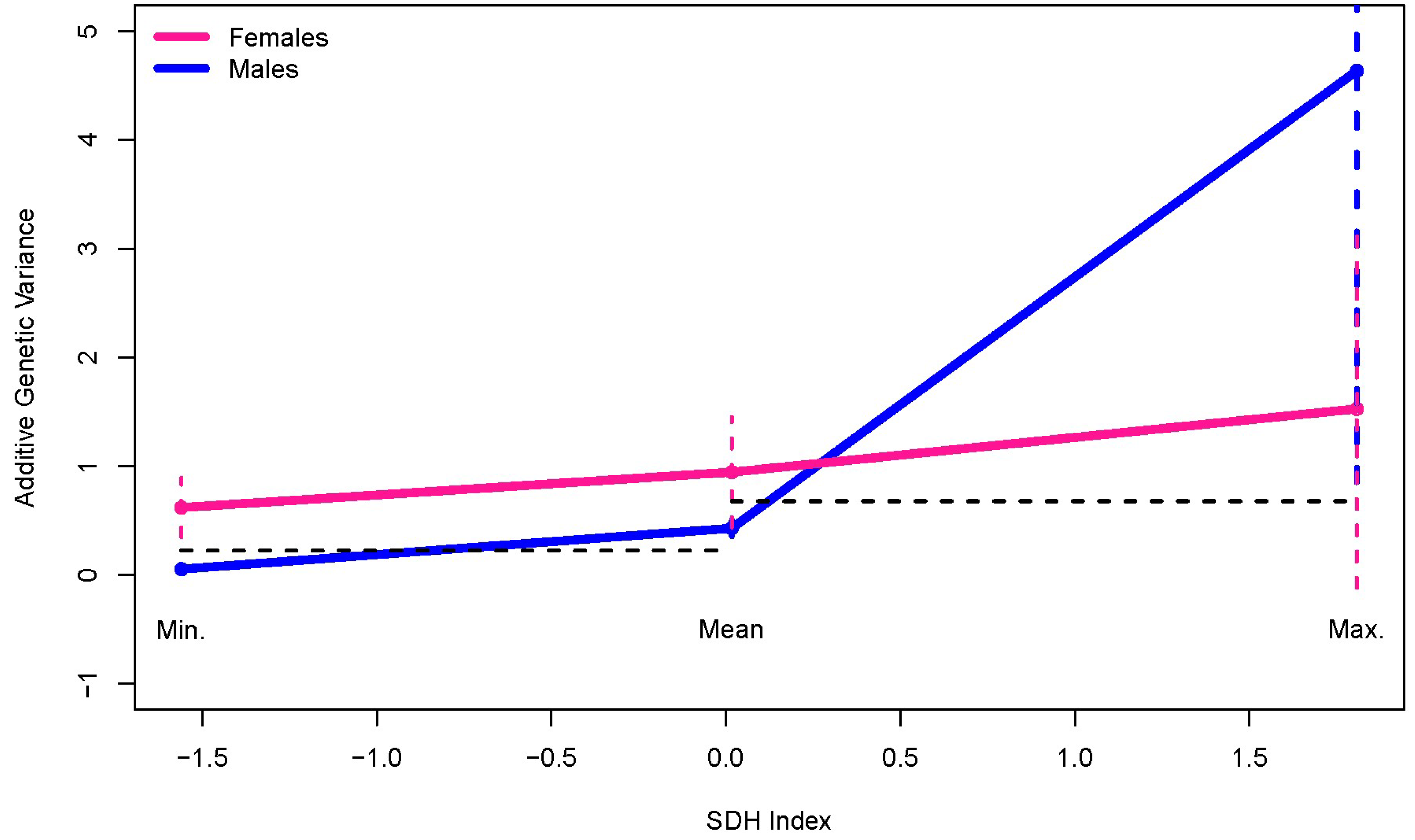
Sex	Additive Genetic Variance	Adjusted Lower Bound *	Adjusted Upper Bound	Wald Statistic	p-Value
Min. SDHI
Females	0.618	0.347	0.890	6.527	0.011
Males	0.053	0.013	0.092
Mean SDHI
Females	0.944	0.437	1.451	1.550	0.213
Males	0.429	0.354	0.503
Max. SDHI
Females	1.5253	−0.1185	3.169	0.6485	0.4206
Males	4.6378	0.8509	8.4247

* See text on the adjusted lower and upper bounds.

; Figure 3). The male and female additive genetic variance functions significantly differed at the minimum SDHI value but not at the mean or maximum. Consistent with the finding of male-specific additive genetic variance heterogeneity (Table 8), the adjusted confidence intervals for the male-specific additive genetic variances do not show overlap when comparing the variances at the minimum to the mean SDHI values and when comparing the variances at the mean to the maximum SDHI values, indicating a sustained and significant increase in the male-specific additive genetic variance with increasing SDHI (Table 9; Figure 3).

4. Conclusions

In this study, we developed a novel model to jointly account for genotype-by-environment interactions for dichotomous and continuous environments. In particular, we applied this joint interaction model to account for the G × Sex and G × SDoH interaction influencing depression. A motivating factor for developing this model is that it allows us to establish if both types of interaction are important independent of one another, similar to the rationale underlying multivariate logistic regression models. We were able to show that there is G × SDoH interaction but only in males and that there is G × Sex interaction due to the cross-sex genetic correlation being significantly different from 1, which indicates that depression is underlain or influenced by different sets of genes in males and females. This model has potentially critical applications in medical research. For example, the dichotomous environment component of the model could be used to model the affected and unaffected states of a given disease of interest, while the continuous environment component could be used to investigate how the genetic response of individuals in both states may be different across a continuous environment of interest, such as physical activity or sedentary behavior. Whatever the case, we are confident that this novel model can lead to fruitful investigations on the genetic basis of response to the environment.

References

- Blangero, J. Statistical genetic approaches to human adaptability. Hum. Biol. 2009, 81, 523–546. [Google Scholar] [CrossRef] [PubMed]
- Viel, K.R.; Warren, D.M.; Buil, A.; Dyer, T.D.; Howard, T.E.; Almasy, L. A comparison of discrete versus continuous environment in a variance components-based linkage analysis of the COGA data. BMC Genet. 2005, 6, S57. [Google Scholar] [CrossRef] [PubMed]
- Avery, C.L.; Freedman, B.I.; Kraja, A.T.; Borecki, I.B.; Miller, M.B.; Pankow, J.S.; Arnett, D.; Lewis, C.E.; Myers, R.H.; Hunt, S.C.; et al. Genotype-by-sex interaction in the aetiology of type 2 diabetes mellitus: Support for sex-specific quantitative trait loci in Hypertension Genetic Epidemiology Network participants. Diabetologia 2006, 49, 2329–2336. [Google Scholar] [CrossRef] [PubMed]
- Winnier, D.A.; Rainwater, D.L.; Cole, S.A.; Williams, J.T.; Dyer, T.D.; Blangero, J.; MacCluer, J.W.; Mahaney, M.C. Sex-specific QTL effects on variation in paraoxonase 1 (PON1) activity in Mexican Americans. Genet. Epidemiol. 2007, 31, 66–74. [Google Scholar] [CrossRef] [PubMed]
- North, K.E.; Franceschini, N.; Borecki, I.B.; Gu, C.C.; Heiss, G.; Province, M.A.; Arnett, D.K.; Lewis, C.E.; Miller, M.B.; Myers, R.H.; et al. Genotype-by-Sex Interaction on Fasting Insulin Concentration: The HyperGEN Study. Diabetes 2007, 56, 137–142. [Google Scholar] [CrossRef]
- Diego, V.P.; de Chaves, R.N.; Blangero, J.; de Souza, M.C.; Santos, D.; Gomes, T.N.; dos Santos, F.K.; Garganta, R.; Katzmarzyk, P.T.; Maia, J.A. Sex-specific genetic effects in physical activity: Results from a quantitative genetic analysis. BMC Med. Genet. 2015, 16, 58. [Google Scholar] [CrossRef]
- Poveda, A.; Chen, Y.; Brändström, A.; Engberg, E.; Hallmans, G.; Johansson, I.; Renström, F.; Kurbasic, A.; Franks, P.W. The heritable basis of gene-environment interactions in cardiometabolic traits. Diabetologia 2017, 60, 442–452. [Google Scholar] [CrossRef]
- Diego, V.P.; Manusov, E.G.; Mao, X.; Almeida, M.; Peralta, J.M.; Curran, J.E.; Mahaney, M.C.; Göring, H.; Blangero, J.; Williams-Blangero, S. Metabolic syndrome traits exhibit genotype-by-environment interaction in relation to socioeconomic status in the Mexican American family heart study. Front. Genet. 2024, 15, 1240462. [Google Scholar] [CrossRef]
- Glahn, D.C.; Kent, J.W., Jr.; Sprooten, E.; Diego, V.P.; Winkler, A.M.; Curran, J.E.; McKay, D.R.; Knowles, E.E.; Carless, M.A.; Göring, H.H.; et al. Genetic basis of neurocognitive decline and reduced white-matter integrity in normal human brain aging. Proc. Natl. Acad. Sci. USA 2013, 110, 19006–19011. [Google Scholar] [CrossRef]
- Arya, R.; Farook, V.S.; Fowler, S.P.; Puppala, S.; Chittoor, G.; Resendez, R.G.; Mummidi, S.; Vanamala, J.; Almasy, L.; Curran, J.E.; et al. Genetic and environmental (physical fitness and sedentary activity) interaction effects on cardiometabolic risk factors in Mexican American children and adolescents. Genet. Epidemiol. 2018, 42, 378–393. [Google Scholar] [CrossRef]
- Pittner, K.; Bakermans-Kranenburg, M.J.; Alink, L.R.A.; Buisman, R.S.M.; van den Berg, L.J.M.; Block, L.H.C.G.C.C.-d.; Voorthuis, A.; Elzinga, B.M.; Lindenberg, J.; Tollenaar, M.S.; et al. Estimating the Heritability of Experiencing Child Maltreatment in an Extended Family Design. Child Maltreatment 2020, 25, 289–299. [Google Scholar] [CrossRef]
- Manusov, E.G.; Diego, V.P.; Sheikh, K.; Laston, S.; Blangero, J.; Williams-Blangero, S. Non-alcoholic Fatty Liver Disease and Depression: Evidence for Genotype × Environment Interaction in Mexican Americans. Front. Psychiatry 2022, 13, 936052. [Google Scholar] [CrossRef] [PubMed]
- Diego, V.P.; Manusov, E.G.; Mao, X.; Curran, J.E.; Göring, H.; Almeida, M.; Mahaney, M.C.; Peralta, J.M.; Blangero, J.; Williams-Blangero, S. Genotype-by-socioeconomic status interaction influences heart disease risk scores and carotid artery thickness in Mexican Americans: The predominant role of education in comparison to household income and socioeconomic index. Front. Genet. 2023, 14, 1132110. [Google Scholar] [CrossRef]
- Marmot, M.G.; Rose, G.; Shipley, M.; Hamilton, P.J. Employment grade and coronary heart disease in British civil servants. J. Epidemiol. Community Health 1978, 32, 244–249. [Google Scholar] [CrossRef] [PubMed]
- Marmot, M.G.; Stansfeld, S.; Patel, C.; North, F.; Head, J.; White, I.; Brunner, E.; Feeney, A.; Marmot, M.G.; Smith, G.D. Health inequalities among British civil servants: The Whitehall II study. Lancet 1991, 337, 1387–1393. [Google Scholar] [CrossRef]
- Langenberg, C.; Shipley, M.J.; Batty, G.D.; Marmot, M.G. Adult Socioeconomic Position and the Association Between Height and Coronary Heart Disease Mortality: Findings From 33 Years of Follow-Up in the Whitehall Study. Am. J. Public Health 2005, 95, 628–632. [Google Scholar] [CrossRef]
- Stringhini, S.; Batty, G.D.; Bovet, P.; Shipley, M.J.; Marmot, M.G.; Kumari, M.; Tabak, A.G.; Kivimäki, M. Association of Lifecourse Socioeconomic Status with Chronic Inflammation and Type 2 Diabetes Risk: The Whitehall II Prospective Cohort Study. PLoS Med. 2013, 10, e1001479. [Google Scholar] [CrossRef] [PubMed]
- Shim, R.S.; Ye, J.; Baltrus, P.; Fry-Johnson, Y.; Daniels, E.; Rust, G. Racial/ethnic disparities, social support, and depression: Examining a social determinant of mental health. Ethn. Dis. 2012, 22, 15–20. [Google Scholar]
- Allen, J.; Balfour, R.; Bell, R.; Marmot, M. Social determinants of mental health. Int. Rev. Psychiatry 2014, 26, 392–407. [Google Scholar] [CrossRef]
- Shim, R.; Koplan, C.; Langheim, F.J.; Manseau, M.W.; Powers, R.A.; Compton, M.T. The social determinants of mental health: An overview and call to action. Psychiatr. Ann. 2014, 44, 22–26. [Google Scholar] [CrossRef]
- World Health Organization. Social Determinants of Mental Health; World Health Organization: Geneva, Switzerland, 2014. [Google Scholar]
- Carod-Artal, F.J. Social Determinants of Mental Health. In Global Mental Health: Prevention and Promotion; Bährer-Kohler, S., Carod-Artal, F.J., Eds.; Springer International Publishing: Cham, Switzerland, 2017; pp. 33–46. [Google Scholar] [CrossRef]
- Alegría, M.; NeMoyer, A.; Falgàs Bagué, I.; Wang, Y.; Alvarez, K. Social Determinants of Mental Health: Where We Are and Where We Need to Go. Curr. Psychiatry Rep. 2018, 20, 95. [Google Scholar] [CrossRef]
- Jeste, D.V.; Koh, S.; Pender, V.B. Perspective: Social Determinants of Mental Health for the New Decade of Healthy Aging. Am. J. Geriatr. Psychiatry 2022, 30, 733–736. [Google Scholar] [CrossRef] [PubMed]
- Jeste, D.V.; Pender, V.B. Social Determinants of Mental Health: Recommendations for Research, Training, Practice, and Policy. JAMA Psychiatry 2022, 79, 283–284. [Google Scholar] [CrossRef] [PubMed]
- Shim, R.S.; Compton, M.T. The Social Determinants of Mental Health: Psychiatrists’ Roles in Addressing Discrimination and Food Insecurity. Focus 2020, 18, 25–30. [Google Scholar] [CrossRef] [PubMed]
- Tafet, G.E.; Nemeroff, C.B. The links between stress and depression: Psychoneuroendocrinological, genetic, and environmental interactions. J. Neuropsychiatry Clin. Neurosci. 2016, 28, 77–88. [Google Scholar] [CrossRef] [PubMed]
- LeMoult, J. From stress to depression: Bringing together cognitive and biological science. Curr. Dir. Psychol. Sci. 2020, 29, 592–598. [Google Scholar] [CrossRef] [PubMed]
- McEwen, B.S.; Akil, H. Revisiting the stress concept: Implications for affective disorders. J. Neurosci. 2020, 40, 12–21. [Google Scholar] [CrossRef] [PubMed]
- McEwen, B.S. Protective and damaging effects of stress mediators: Central role of the brain. Dialogues Clin. Neurosci. 2022, 8, 367–381. [Google Scholar] [CrossRef] [PubMed]
- McEwen, B.S. Physiology and Neurobiology of Stress and Adaptation: Central Role of the Brain. Physiol. Rev. 2007, 87, 873–904. [Google Scholar] [CrossRef]
- McEwen, B.S. Neurobiological and Systemic Effects of Chronic Stress. Chronic Stress 2017, 1, 2470547017692328. [Google Scholar] [CrossRef]
- Wilkinson, R.G.; Marmot, M. Social Determinants of Health: The Solid Facts; World Health Organization: Geneva, Switzerland, 2003. [Google Scholar]
- Kang, H.-J.; Park, Y.; Yoo, K.-H.; Kim, K.-T.; Kim, E.-S.; Kim, J.-W.; Kim, S.-W.; Shin, I.-S.; Yoon, J.-S.; Kim, J.H. Sex differences in the genetic architecture of depression. Sci. Rep. 2020, 10, 9927. [Google Scholar] [CrossRef] [PubMed]
- Labonté, B.; Engmann, O.; Purushothaman, I.; Menard, C.; Wang, J.; Tan, C.; Scarpa, J.R.; Moy, G.; Loh, Y.-H.E.; Cahill, M. Sex-specific transcriptional signatures in human depression. Nat. Med. 2017, 23, 1102–1111. [Google Scholar] [CrossRef] [PubMed]
- Seney, M.L.; Glausier, J.; Sibille, E. Large-scale transcriptomics studies provide insight into sex differences in depression. Biol. Psychiatry 2022, 91, 14–24. [Google Scholar] [CrossRef] [PubMed]
- Silveira, P.P.; Pokhvisneva, I.; Howard, D.M.; Meaney, M.J. A sex-specific genome-wide association study of depression phenotypes in UK Biobank. Mol. Psychiatry 2023, 28, 2469–2479. [Google Scholar] [CrossRef] [PubMed]
- Lee, K.; Kim, D.; Cho, Y. Exploratory Factor Analysis of the Beck Anxiety Inventory and the Beck Depression Inventory-II in a Psychiatric Outpatient Population. J. Korean Med. Sci. 2018, 33, e128. [Google Scholar] [CrossRef]
- Penley, J.A.; Wiebe, J.S.; Nwosu, A. Psychometric properties of the Spanish Beck Depression Inventory-II in a medical sample. Psychol. Assess. 2003, 15, 569–577. [Google Scholar] [CrossRef] [PubMed]
- Wiebe, J.S.; Penley, J.A. A psychometric comparison of the Beck Depression Inventory-II in English and Spanish. Psychol. Assess. 2005, 17, 481–485. [Google Scholar] [CrossRef] [PubMed]
- Wang, Y.P.; Gorenstein, C. Psychometric properties of the Beck Depression Inventory-II: A comprehensive review. Braz. J. Psychiatry 2013, 35, 416–431. [Google Scholar] [CrossRef] [PubMed]
- Billioux, A.; Verlander, K.; Anthony, S.; Alley, D. Standardized screening for health-related social needs in clinical settings: The accountable health communities screening tool. In NAM Perspectives; National Academy of Medicine: Washington, DC, USA, 2017. [Google Scholar]
- Lange, K. Mathematical and Statistical Methods for Genetic Analysis; Springer: Berlin/Heidelberg, Germany, 2002; Volume 488. [Google Scholar]
- Blangero, J.; Diego, V.P.; Dyer, T.D.; Almeida, M.; Peralta, J.; Kent, J.W., Jr.; Williams, J.T.; Almasy, L.; Göring, H.H. A kernel of truth: Statistical advances in polygenic variance component models for complex human pedigrees. Adv. Genet. 2013, 81, 1–31. [Google Scholar] [CrossRef]
- Diego, V.P.; Kent, J.W.; Blangero, J. Familial Studies: Genetic Inferences. In International Encyclopedia of the Social & Behavioral Sciences, 2nd ed.; Wright, J.D., Ed.; Elsevier: Oxford, UK, 2015; pp. 715–724. [Google Scholar] [CrossRef]
- Sorensen, D.; Gianola, D. Likelihood, Bayesian and MCMC Methods in Quantitative Genetics; Springer: Berlin/Heidelberg, Germany, 2002. [Google Scholar]
- Quillen, E.E.; Voruganti, V.S.; Chittoor, G.; Rubicz, R.; Peralta, J.M.; Almeida, M.A.; Kent, J.W., Jr.; Diego, V.P.; Dyer, T.D.; Comuzzie, A.G.; et al. Evaluation of estimated genetic values and their application to genome-wide investigation of systolic blood pressure. BMC Proc. 2014, 8, S66. [Google Scholar] [CrossRef]
- Almasy, L.; Blangero, J. Multipoint quantitative-trait linkage analysis in general pedigrees. Am. J. Hum. Genet. 1998, 62, 1198–1211. [Google Scholar] [CrossRef] [PubMed]
- Self, S.G.; Liang, K.-Y. Asymptotic Properties of Maximum Likelihood Estimators and Likelihood Ratio Tests under Nonstandard Conditions. J. Am. Stat. Assoc. 1987, 82, 605–610. [Google Scholar] [CrossRef]
- Dominicus, A.; Skrondal, A.; Gjessing, H.K.; Pedersen, N.L.; Palmgren, J. Likelihood ratio tests in behavioral genetics: Problems and solutions. Behav. Genet. 2006, 36, 331–340. [Google Scholar] [CrossRef] [PubMed]
- Visscher, P.M. A note on the asymptotic distribution of likelihood ratio tests to test variance components. Twin. Res. Hum. Genet. 2006, 9, 490–495. [Google Scholar] [CrossRef] [PubMed]
- DasGupta, A. Asymptotic Theory of Statistics and Probability; Springer: Berlin/Heidelberg, Germany, 2008; Volume 180. [Google Scholar]
- Giampaoli, V.; Singer, J.M. Likelihood ratio tests for variance components in linear mixed models. J. Stat. Plan. Inference 2009, 139, 1435–1448. [Google Scholar] [CrossRef]
- Azzalini, A. Statistical Inference Based on the Likelihood; Routledge: London, UK, 2017. [Google Scholar]
- Edwards, A.W.F. Likelihood: An Account of the Statistical Concept of Likelihood and Its Application to Scientific Inference; Johns Hopkins University Press: Baltimore, MA, USA, 1992. [Google Scholar]
- Held, L.; Bové, D.S. Likelihood and Bayesian Inference. Statistics for Biology and Health; Springer: Berlin/Heidelberg, Germany, 2020. [Google Scholar]
- Pawitan, Y. All Likelihood: Statistical Modelling and Inference Using Likelihood; Oxford University Press: Oxford, UK, 2001. [Google Scholar]
- Severini, T.A. Likelihood Methods in Statistics; Oxford University Press: Oxford, UK, 2000. [Google Scholar]
- Neudecker, H.; Trenkler, G. On the approximate variance of a nonlinear function of random variables. In Contributions to Probability and Statistics: Applications and Challenges; World Scientific: Singapore, 2006; pp. 172–177. [Google Scholar]
- Nakagawa, S.; Cuthill, I.C. Effect size, confidence interval and statistical significance: A practical guide for biologists. Biol. Rev. 2007, 82, 591–605. [Google Scholar] [CrossRef] [PubMed]
- Julious, S.A. Using confidence intervals around individual means to assess statistical significance between two means. Pharm. Stat. 2004, 3, 217–222. [Google Scholar] [CrossRef]
- Knol, M.J.; Pestman, W.R.; Grobbee, D.E. The (mis)use of overlap of confidence intervals to assess effect modification. Eur. J. Epidemiol. 2011, 26, 253–254. [Google Scholar] [CrossRef] [PubMed]
- Maghsoodloo, S.; Huang, C.-Y. Comparing the overlapping of two independent confidence intervals with a single confidence interval for two normal population parameters. J. Stat. Plan. Inference 2010, 140, 3295–3305. [Google Scholar] [CrossRef]
- Molenberghs, G.; Verbeke, G. Likelihood Ratio, Score, and Wald Tests in a Constrained Parameter Space. Am. Stat. 2007, 61, 22–27. [Google Scholar] [CrossRef]
- Elston, R.; Rao, D. Statistical modeling and analysis in human genetics. Annu. Rev. Biophys. Bioeng. 1978, 7, 253–286. [Google Scholar] [CrossRef] [PubMed]
- Lange, K.; Westlake, J.; Spence, M.A. Extensions to pedigree analysis III. Variance components by the scoring method. Ann. Hum. Genet. 1976, 39, 485–491. [Google Scholar] [CrossRef] [PubMed]
- Kirkpatrick, M.; Heckman, N. A quantitative genetic model for growth, shape, reaction norms, and other infinite-dimensional characters. J. Math. Biol. 1989, 27, 429–450. [Google Scholar] [CrossRef] [PubMed]
- Pletcher, S.D.; Geyer, C.J. The genetic analysis of age-dependent traits: Modeling the character process. Genetics 1999, 153, 825–835. [Google Scholar] [CrossRef]
- Jaffrézic, F.; Pletcher, S.D. Statistical models for estimating the genetic basis of repeated measures and other function-valued traits. Genetics 2000, 156, 913–922. [Google Scholar] [CrossRef]
- Pletcher, S.D.; Jaffrézic, F. Generalized character process models: Estimating the genetic basis of traits that cannot be observed and that change with age or environmental conditions. Biometrics 2002, 58, 157–162. [Google Scholar] [CrossRef]